Correlation of black hole and bulge masses: driven by energy but correlated with momentum

Abstract

We use a recent sample of 49 galaxies to show that there is a proportionality relation between the black hole mass $M_{\rm BH}$ and the quantity $\mu\equiv M_{\rm G}\sigma/c$, where $M_{\rm G}$ is mass of the spheroidal stellar component and $\sigma$ is the stellar velocity dispersion. $\mu$ is called the momentum parameter and the ratio is $M_{\rm BH}/\mu\approx 3.3$. This result is applied to the penetrating-jet feedback model which argues that the correlation that holds is with a momentum-like parameter, although this feedback mechanism is based on energy balance.

1 Introduction

Relations between a supermassive black hole (SMBH) mass, $M_{\rm BH}$, and other properties of its host galaxy have been studied intensively in the last decade. Two of the galactic properties most commonly correlated with $M_{\rm BH}$ are the stellar mass of the spheroidal component (which we refer to as the bulge), $M_{\rm G}$ (e.g. Kormendy & Richstone 1995; Magorrian et al. 1998; Laor 2001; Hu 2009; Graham & Spitler 2009), and it’s stellar velocity dispersion, $\sigma$ (e.g. Gebhardt et al. 2000; Merritt & Ferrarese 2001; Graham 2008a; Graham (2008b); Hu 2008; Shen et al. 2008; Gültekin et al. 2009). These relations are often assumed to have the form of a power law (i.e. linear when plotted on a log-log scale). However, due to the large scatter there is still no consensus on the best parameters of the different relations. For example, despite some claims for a proportionality relation between the SMBH and bulge mass, Laor (2001) found that the ratio $M_{\rm BH}/M_{\rm G}$ increases with mass. This conclusion was strengthened by some models and simulations (e.g. Shabala & Alexander 2009).

The more significant disagreement is on which fundamental galactic property is behind the correlations. In a recent paper, Feoli et al. (2010) studied three samples of SMBH masses and their host galaxies. They argued that $M_{\rm BH}$ is better correlated with the energy parameter, $M_{\rm G}\sigma^{2}$, than with $M_{\rm G}$ or with $\sigma$ alone. Behind this comparison stands the view that the feedback between the accreting SMBH and its environment is driven by energy.

Results from recent years show that the process of galaxy formation requires another energy source to that of the gravitational energy of the galaxy, not only to heat the gas, but also to expel large quantities of it out of the galaxy (e.g. Bower et al. 2008). Momentum in the relativistic jets alone is not sufficient to expel (accelerate to escape velocity, $\sim$ few $\sigma$) a considerable amount of mass ($\ga M_{\rm G}$). The maximum momentum that can be released in a relativistic jet (which is the expected case for an outflow launched by BH accretion), $\eta M_{\rm BH}c$, is generally smaller than $M_{\rm G}\sigma$, the approximate momentum needed to expel large quantities of gas.

Silk & Nusser (2010) argue that radiation momentum is also incapable of accounting for the correlation. Let us consider King (2003) as an example of a model based on expulsion of gas by radiation momentum. In that model, an expression for the BH mass is derived (equation 15 there) where a mass of $M_{\rm BH}=1.5\times 10^{8}~{}{\rm M}_{\odot}$ is obtained for $\sigma=200~{}\rm{km}~{}{\rm s}^{-1}$. For this value of $\sigma$, the gas mass inside a typical radius of $10~{}\rm{kpc}$ is found to be $3\times 10^{10}~{}{\rm M}_{\odot}$ according to King’s equation (4). If this is the amount of gas expelled by radiation momentum $M_{\rm expel}$, then the ratio of the expelled mass to the BH mass is $M_{\rm expel}/M_{\rm BH}\sim 200$. while from This ratio from observations it is in fact $\sim 500$. This ratio is probably even much lower in King’s model as he takes the cosmological value of 0.16 for the baryon fraction, whereas this fraction is much larger (even close to unity) in the bulges of spiral galaxies. Another problem (though less severe) with this model is that one does not expect the ransfer of radiation momentum to mechanical momentum to be 100 per cent efficient. Thus, we conclude that radiation momentum can expel only a small amount of gas, and that the correlation cannot be explained in King’s model.

On the other hand, there is more than enough energy released from the accretion process to expel the gas (by a factor of $\sim 50$), or $\eta M_{\rm BH}c^{2}\gg M_{\rm G}\sigma^{2}$. The problem with energy is the opposite: if deposition of jets’ energy into the ISM is too efficient, almost no star formation will occur.

Thus, a successful theory should be based on a feedback mechanism in which the deposition of the jets’ energy to the ISM is regulated; it should also be able to derive the mathematical form of the SMBH–galaxy relation from the basic properties of the galaxy and its active galactic nucleolus (AGN). The penetrating-jet feedback mechanism (Soker, 2009) has these two attributes. In this model, the energy transfer from the jets to the ISM is efficient enough to expel large amounts of gas and suppress star formation only when the jets are stopped within the bulge, and do not propagate to large distances by penetrating through the ISM. Soker (2009) found that this requirement leads to a proportionality relation between the BH mass and the momentum parameter

$$\mu\equiv M_{\rm G}\frac{\sigma}{c}$$ (1)

as detailed in Section 2.

Motivated by the recent data and the penetrating-jet feedback mechanism, we carry out the present study. In Section 3 we examine the correlation between $M_{\rm BH}$ and $\mu$. We ignore the differences between elliptical galaxies, classical bulges and pseudo-bulges (e.g. Gadotti & Kauffmann 2009; Nowak et al. 2010; Hu 2009). In Section 4 we apply the results to the jet penetrating model and derive the approximate amount of momentum carried by the jets. We summarize in Section 5.

2 The penetrating-jet feedback mechanism

In the penetrating-jet feedback mechanism the energy transfer from the jets is efficient enough to expel large amounts of gas and suppress star formation only when the jets are stopped within the bulge, and do not propagate to large distances by penetrating into through the gas. The condition for jet-stopping is that the time required for the jet to propagate through the surrounding gas and break out of it must be longer than the jet crossing time (the time it takes a blob of material to transverse the jet’s width). This situation is analogous to an attempt to pierce a hole through a plank of wood with a drill, when the drill moves horizontally and does not stay over one spot for enough time. This is referred to as the non-penetration condition.

Mathematically, the jet crossing time at a typical radius $r_{\rm s}$ (where the cooling surrounding mass $M_{\rm s}$ resides) is

$$\tau_{\rm c}\equiv\frac{2r_{\rm s}\tan{\theta}}{v_{\rm rel}}\approx\frac{2r_{\rm s}\theta}{v_{\rm rel}}$$ (2)

where $\theta$ is the half opening angle of the jet and $v_{\rm rel}$ is the relative transverse motion between the inflowing mass and the SMBH ($v_{\rm rel}\sim\sigma$). We assumes the jet to be narrow, thus $\tan\theta\approx\theta$.

The penetration time is $\tau_{\rm p}\equiv r_{\rm s}/v_{\rm h}$ where $v_{\rm h}$ is the velocity of the head of the jet, which is derived from momentum balance (ram pressure balance of the jet and the ambient gas), and is given by

$$v_{\rm h}=\sqrt{\frac{2\dot{M}_{\rm f}v_{\rm f}\sigma}{\dot{M}_{\rm s}\theta^{2}}},$$ (3)

where the subscript ‘f’ (for ‘flow’) is used to denote magnitudes associated with the jets (thus $\dot{M}_{\rm f}$ is the mass outflow rate of the two jets together and $v_{\rm f}$ is its velocity). $\dot{M}_{\rm s}$ is the mass inflow rate from $\sim 1~{}\rm{kpc}$ scale. Equation (3) was derived under the assumptions of: supersonic motion, $v_{\rm f}\gg v_{\rm h}$, and the stronger assumption that the inflowing speed of $\dot{M}_{\rm s}$ is $\sigma$.

The non-penetration condition $\tau_{\rm c}\lesssim\tau_{\rm p}$ leads to the following inequality

$$\dot{M}_{\rm s}\gtrsim\frac{\sigma c}{v_{\rm rel}^{2}}8\eta_{p}\dot{M}_{\rm BH}$$ (4)

where $\eta_{p}$ relates the rate of mass outflow $\dot{M}_{\rm f}$ to the rate of accretion or BH growth $\dot{M}_{\rm BH}$

$$\dot{p}_{\rm f}\equiv\dot{M}_{\rm f}v_{\rm f}\equiv\eta_{p}\dot{M}_{\rm BH}c.$$ (5)

$\dot{p}_{\rm f}$ is the rate of momentum carried by the two jets (that we term momentum discharge). Note that equation (5) is equivalent to the familiar relation for the total energy transfer

$$\dot{E}_{\rm BH}=\eta\dot{M}_{\rm BH}c^{2},$$ (6)

where $\dot{E}_{\rm BH}$ is the total energy released by the BH per unit time, and $\eta\approx 0.1$ is the accretion efficiency. The total energy is released in both radiation and mechanical energy of the jets. The fraction of kinetic energy carried by the jets is considered in Section 4.

Equation (4) must in fact be an approximate equality: if the inflow rate is above the value of the right hand side, the deposition of energy by the jets is efficient enough to expel the mass back to large distances and heat it. The inflowing mass that is not expelled by the jets is assumed to form stars in the bulge. Thus, time integration of both sides of the equation (4) (with equality sign; we also substitute $v_{\rm rel}=\sigma$), leads to the following relation (Soker 2009, 2010)

$$M_{\rm BH}=\frac{1}{8\eta_{p}}\mu,$$ (7)

where $\mu$ is the momentum parameter (defined in equation 1) which has units of mass.

Feedback mechanisms have been discussed by many authors in the past, both to suppress gas cooling in cooling flow clusters (e.g. Binney & Tabor 1995; Nulsen & Fabian 2000; Reynolds et al. 2002; Omma & Binney 2004; Soker & Pizzolato 2005) and to suppress star formation during galaxy formation (e.g. Silk & Rees 1998; Fabian 1999; King 2003; Croton et al. 2006; Bower et al. 2008; Shabala & Alexander 2009; Soker 2009, 2010). The penetrating-jet feedback mechanism does not make use of the Eddington luminosity limit, while some authors do (e.g. Silk & Rees 1998; King 2003). Most models (e.g. Silk & Rees 1998; Fabian 1999) do not consider the geometry explicitly, while in the penetrating-jet feedback mechanism the geometry of the narrow jets and the motion of their source are key issues; these introduce the factor $1/8$ in equation (7).

In the penetrating-jet feedback mechanism, the fast jets have two modes of interaction with the surrounding gas: if the jets penetrate through the ISM gas, they deposit most of their energy at large distances, and thus cannot expel gas; if they cannot penetrate, they are shocked, and a hot bubble is formed. If the radiative cooling time of the hot bubble is longer than the flow time (or acceleration time), it efficiently accelerates the surrounding gas and expels it. Namely, in order to suppress star formation it is necessary that the jets do not penetrate through the ISM. For that, the jets should encounter new material before they escape. This requires that there is a transverse velocity component between the jets and the ambient gas with which it interacts. The physical condition for efficient expulsion of the gas is that the typical time for the jets–ISM relative motion to cross the jet’s width in the transverse motion at a radius $r_{s}$ (from the central source) should be shorter than the penetration time at radius $r_{s}$.

3 The correlation

3.1 Methods and Sample

The $M_{\rm BH}$–$\mu$ relation is initially assumed to be a power law of the form

$$\log_{10}M_{\rm BH}=\alpha+\beta\log_{10}\mu.$$ (8)

We use a least squares estimator of linear relations like fitexy of Press et al. (1992), that takes into account measurement errors in both coordinates. Like Tremaine et al. (2002), we add a constant residual error $\epsilon_{0}$ (intrinsic scatter) until $\chi_{r}^{2}=1$ is obtained (see appendix). However, while Tremaine et al. (2002) have assumed the intrinsic scatter to be on the BH mass alone, we consider other possibilities as detailed below. Novak et al. (2006) found based on Monte Carlo simulations that this method estimates the slope with the least bias and variance. The maximum likelihood estimator used by Gültekin et al. (2009) gives similar results to the above, but there is no freedom to manually set $\epsilon_{0}$ and study how it changes the results. The ability to vary $\epsilon_{0}$ (or alternatively, $\chi_{r}^{2}$) is important because the result of the fit is sensitive to the stated measurement errors. First we use this method to show that the slope $\beta$ of the relation in study is reasonably close to 1, and later we force $\beta=1$ and find the intercept $\alpha$.

We use three models for the intrinsic scatter: in the $y$-scatter model we assume (like Tremaine et al. 2002) that $\epsilon_{0}$ is the residual variance in $\log_{10}M_{\rm BH}$ (which is traditionally the $y$ coordinate); in the $x$-scatter model, $\epsilon_{0}$ is the scatter in the galactic property in question, in our case $\log_{10}\mu$; in the orthogonal scatter model, residual errors are added to both coordinates, such that the combined error is $\epsilon_{0}$ in the direction perpendicular to the ridge line of the relation. The estimators of the three models are given in the appendix. The actual value of $\epsilon_{0}$ is meaningful only within the three models, and it is generally wrong to compare the values obtain from each one. We also note that the assumption that the scatter (in whatever direction) is constant throughout the relation is made out of ignorance and may not represent the real situation.

It is impossible to avoid specifying the direction of the intrinsic scatter (Novak et al., 2006), and an extremely biased result is obtained if the calculation is performed under the assumptions that the residual variance is in the wrong coordinate. It is also claimed by Novak et al. (2006) that the direction of the scatter depends on whether it was the BH which affected the host galaxy property or vice versa. In the penetrating-jet feedback mechanism, the former is true (because the jets launched by the BH affect the gas in the galaxy), and thus the $x$-scatter model better suits the theory. However, acknowledging that both $M_{\rm BH}$ and the momentum parameter are affected in a non trivial manner by phenomena such as mergers, we do not give the $x$-scatter model any preference, and regard the orthogonal scatter model as a compromise between the other two.

For simplicity we use the S sample of Gültekin et al. (2009), which includes 49 measured BH masses but no upper limits. In that paper, two different mass measurements are stated for both NGC1399 and NGC5128; we take the (geometric) average mass of each one, and the uncertainty ranges are combined. The $M_{\rm G}$ values are taken from table 3 in Feoli et al. (2010).

Since our estimators cannot deal with asymmetric measurement errors, we adopt the common practice of taking

$$\delta y={\textstyle\frac{1}{2}}\left[\log_{10}M_{\rm high}-\log_{10}M_{\rm low}\right]$$ (9)

where $\delta y$ is the uncertainty in the logarithmic BH mass, and $M_{\rm high}$ and $M_{\rm low}$ are the published limits of the 68 per cent confidence region. The error on all $M_{\rm G}$ values is taken to be 0.18 dex; this dominates over the error in $\sigma$ (which is typically $\sim 0.02$ dex) in the uncertainty in momentum parameter.

3.2 Results

Fig. 1 shows the best fitting slope obtained for equation (8) using the three different scatter models, as a function of the achieved $\chi_{r}^{2}$. The solid line is the $x$-scatter model (scatter in the momentum parameter), the dotted line is the orthogonal scatter model, and the dashed line is the $y$-scatter model (scatter in the SMBH mass). In the point on the right where the three lines meet, $\chi^{2}$ is maximal and there is no residual variance in any direction ($\epsilon_{0}=0$). The two vertical lines mark the 68 per cent confidence interval of the (reduced) $\chi^{2}$-distribution with 47 degrees of freedom, centred at $\chi_{r}^{2}=1$. The best fitting values for $\alpha$ and $\beta$ for $\chi_{r}^{2}=1$, and the obtained $\epsilon_{0}$, are given in Table 1. While the values of $\alpha$ vary greatly and have large errors, the errors on all slopes are at the $\sim 8$ per cent level, and all are consistent with 1 to within two standard deviations.

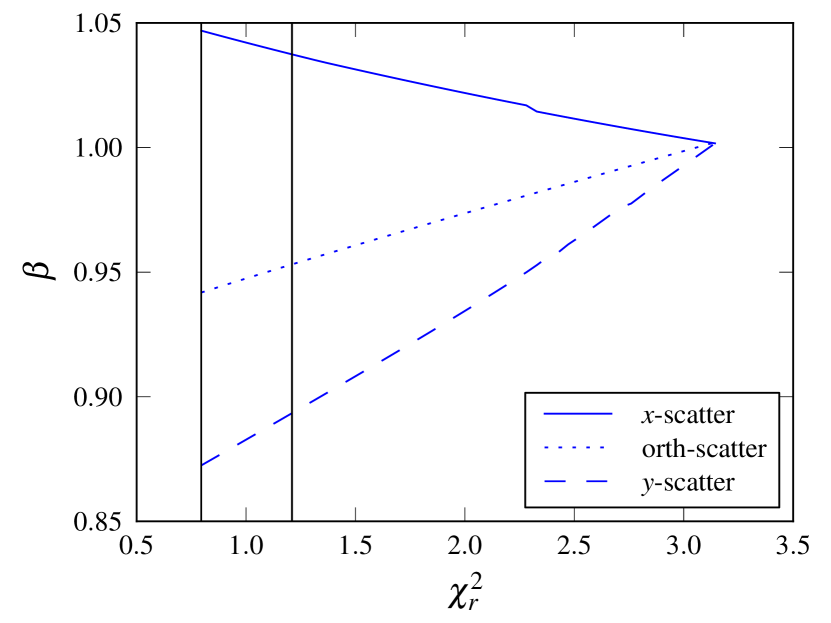
Figure 1: The best fitting slope $\beta$ in equation (8) as a function of the demanded $\chi_{r}^{2}$ in the three scatter models. The solid line is the $x$-scatter model, the dotted line is the orthogonal scatter model, and the dashed line is the $y$-scatter model. The two vertical lines mark the 68 per cent confidence interval of the (reduced) $\chi^{2}$-distribution with 47 degrees of freedom, centred at $\chi_{r}^{2}=1$. Note that this interval does not actually give the uncertainty on $\beta$, which is calculated according to the algorithm of Press et al. (1992). The best fitting slope and intercept for $\chi_{r}^{2}=1$ are given in Table 1.

Table 1: The best fitting values for equation (8) in the three models of intrinsic scatter. In all models, $\epsilon_{0}$ was increased until $\chi_{r}^{2}=1$ was achieved. The values for the intercept $\alpha$ vary greatly and have large errors, but all slopes are consistent with 1 to within two standard deviations. Note that $\epsilon_{0}$ has a somewhat different meaning in each model (see text), and does not indicate goodness-of-fit.

Model	$\alpha\pm\delta\alpha$	$\beta\pm\delta\beta$	$\epsilon_{0}$
$x$-scatter	$0.2\pm 0.6$	$1.04\pm 0.08$	0.32
$y$-scatter	$1.4\pm 0.5$	$0.88\pm 0.07$	0.31
orth-scatter	$0.9\pm 0.6$	$0.95\pm 0.08$	0.32

This result justifies trying to modify the assumption that the $M_{\rm BH}$–$\mu$ relation is a power law, and instead assume that it is a linear relation ($\beta\equiv 1$). We used a similar method to fitexy to obtain $\alpha$, as detailed in the Appendix. The forcing of the slope to 1 renders the three scatter models equivalent. The residual error is taken to be the average value obtained in Table 1. The resulting intercept is

$$\alpha=0.51\pm 0.07.$$ (10)

The uncertainty in $\alpha$ is obtained using this method is much smaller than before, because there is much less freedom to change $\alpha$ while minimizing $\chi^{2}$. The SMBH mass is plotted as a function of the momentum parameter in Fig. 2, where the best fitting lines are also shown. The solid line corresponds to the $x$-scatter model, the dashed line corresponds to the $y$-scatter model, and the dotted line has a fixed slope set to $\beta=1$ and an intercept given by equation (10).

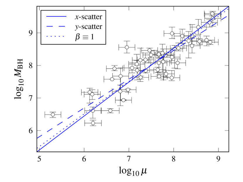
Figure 2: The $M_{\rm BH}$–$\mu$ correlation. $\mu$ is the momentum parameter defined in equation (1). Both axes are logarithmic in $\rm{M}_{\odot}$. The data from the Gültekin et al. (2009) S sample. The solid line and the dashed line are the best fitting straight lines according to the $x$- and $y$-scatter models respectively. The dotted line here has a slope of $\beta=1$ and the intercept is given by equation (10).

The motivation to check the $M_{\rm BH}$–$\mu$ correlation comes from the penetrating-jet feedback mechanism that gives both the slope $\beta$ and the intercept $\alpha$ from basic parameters of the systems; one of these parameters is determined here (see Section 4). Other models exist, but in many the slope and/or the intercept are not given from basic parameters of the system. Hopkins et al. (2007), for example, take the accretion rate based on an Eddington-limited prescription based on Bondi-Hoyle-Lyttleton accretion theory. The Bondi-Hoyle-Lyttleton accretion theory has the disadvantage that it cannot maintain a feedback in real time (Soker, 2010). Their theoretical explanation is based on pressure-driven wind, and they expect a relation of the form $M_{\rm BH}\propto M_{\rm G}^{1/2}\sigma^{2}$. This is not compatible with observations, as they themselves find.

3.3 Comparison

We wish to compare the $M_{\rm BH}$–$\mu$ correlation we showed with correlations with other quantities such as $\sigma$. However, by setting $\chi_{r}=1$ to account for the intrinsic scatter, one makes it impossible to use common goodness of fit tests. $\epsilon_{0}$ itself would be a fair indicator of goodness of fit only if the scatter is in the same quantity, i.e. $M_{\rm BH}$, in each relation; but we have no good indication that that is the case. Let us nevertheless investigate other relations using the same fitting method described in Section 3.1 and the $y$-scatter model (so that the scatter is in the BH mass). We use the same dataset and assume all relations we test have the same form as equation (8).

Table 2 gives the slope (with formal error) and the intrinsic scatter for different popular relations. The slopes were calculated with the $y$-scatter model, which we do not prefer, so that the scatter is in $\log_{10}M_{\rm BH}$ in all tested correlations. We note that our results for the $M_{\rm BH}$–$\sigma$ relation are very close, but not identical, to those appearing in table 6 of Gültekin et al. (2009), where $\beta=4.06\pm 0.37$ and $\epsilon_{0}=0.40$ (third row there, titled T02ind). These numbers were obtained using the same method and data. However, it is possible that the discrepancy comes from different treatment of NGC1399 and NGC5128 (the galaxies with two $M_{\rm BH}$ measurements for each); Gültekin et al. (2009) take all measurement and give each one half the weight, while in this work we average the values and expand the uncertainty ranges. We note that the sample of Gültekin et al. (2009) is basically the same as that of Graham (2008b), who find the slope to be 4.28, which is somewhat closer to the value we find.

All values of $\epsilon_{0}$ for the tested correlations are comparable; we give a crude estimate of the error in $\epsilon_{0}$ to be $\approx 0.05$ in all four cases. This is determined by using the formula

$$\delta\epsilon_{0}={\textstyle\frac{1}{2}}[\epsilon_{0}(\chi_{\rm low}^{2})-\epsilon_{0}(\chi_{\rm high}^{2})],$$ (11)

where $\epsilon_{0}(\chi_{\rm low}^{2})$ is the intrinsic scatter that produces a $\chi^{2}$ at the low limit of the 68 per cent confidence range of the $\chi^{2}$-distribution (shown in Fig. 1); $\epsilon_{0}(\chi_{\rm high}^{2})$ corresponds to the high limit of this range. The formal error in the scatter in the $M_{\rm BH}$–$\sigma$ relation as found by Gültekin et al. (2009) using their maximum likelihood method is $\approx 0.06$.

Given that the shape of the scatter is unknown and that the assumptions made were very simplistic, the uncertainty in $\epsilon_{0}$ may be much higher than our estimate. Thus, all tested correlations seem to be equally good.

Table 2: The slope (with error) and intrinsic scatter in correlations of the BH mass with four parameters. All relations are assumed to be linear in the log-log plane. The results were obtained using the $y$-scatter model, which we do not prefer. The estimated error in $\epsilon_{0}$ in all cases is 0.05 (see text), indicating that all correlations are equally good for the current data.

Parameter	$\beta\pm\delta\beta$	$\epsilon_{0}$
$\mu$	$0.88\pm 0.07$	$0.31$
$\sigma$	$4.18\pm 0.37$	$0.38$
$M_{\rm G}$	$1.07\pm 0.09$	$0.33$
$M_{\rm G}\sigma^{2}$	$0.74\pm 0.05$	$0.31$

4 implications for the penetrating-jet feedback mechanism

We now use the results of Section 3.2 to estimate the value of $\eta_{p}$. We recall that $\eta_{p}$ is defined in equations (7) and (5), and is the ratio of the momentum discharge carried to $\dot{M}_{\rm BH}c$. Assuming a proportionality relation between $M_{\rm BH}$ and $\mu$, the ratio is $M_{\rm BH}/\mu=10^{\alpha}=3.26\pm 0.51$ according to equation (10). Substituting this value in equation (7) gives

$$\eta_{p}=0.038\pm 0.006.$$ (12)

We thus derived the average value of a fundamental parameter characterizing jets launched by an AGN during the phase of SMBH growth at galaxy formation.

From equations (5) and (6) it is possible to derive the fraction $f$ of the total energy that is carried by the jets. Namely, the kinetic power of the jets divided by the total power of the accreting SMBH as given by equation (6). Substituting the relativistic expressions for the jets’ kinetic energy and momentum, we find

$$f=\frac{\dot{E}_{k,\rm f}}{\dot{E}_{\rm BH}}=\frac{\eta_{p}}{\eta}\frac{c}{v_{\rm f}}\left(1-\sqrt{1-\frac{v_{\rm f}^{2}}{c^{2}}}\right)$$ (13)

where $v_{\rm f}$ is the velocity of the jets. In the relativistic limit ($v_{\rm f}\rightarrow c$), the fraction $f$ of kinetic energy approaches a constant ${\eta_{p}}/{\eta}=0.38$ (for $\eta=0.1$); in the non-relativistic limit ($v\lesssim 0.5c$) equation (13) becomes $f=\frac{\eta_{p}}{2\eta}\frac{v_{\rm f}}{c}$. Namely, in the relativistic limit and during the phase of SMBH growth and galaxy formation, the jets carry an average $\sim 0.4$ of the SMBH power, while in the non relativistic limit it is a small fraction.

There is a lower limit set by the requirement that the jets have enough energy to expel the required amount of gas from the newly formed galaxy; the requirement is that $E_{k,\rm f}\ga\frac{1}{2}M_{\rm G}\sigma^{2}$, or

$$f\ga\frac{M_{\rm G}\sigma^{2}}{2\eta M_{\rm BH}c^{2}}.$$ (14)

Using the same typical numbers as in Section 1, we find $f\ga 0.002$. This is an important result: even if the jets are not relativistic and carry only a small fraction of the energy, then this mechanism can work. Non-relativistic wide outflows, termed slow massive wide (SMW) outflows, can be formed by disk winds instead of highly relativistic jets from very close to the SMBH, or from a narrow relativistic jet that very close to the SMBH turns into a non-relativistic jet by interacting with the ambient material (Soker, 2008).

Let us elaborate on SMW outflows. Feedback based on slow ($\sim 10^{4}~{}\rm{km}~{}{\rm s}^{-1}$) massive wide jets has been applied in cooling flow clusters (Sternberg et al. 2007; Soker et al. 2010) and in elliptical galaxies (Ostriker et al., 2010) to heat and expel gas. The properties of such SMW outflows have been recently deduced (Moe et al. 2009; Dunn et al. 2010). For these outflows to be energetic, they must result from accretion close to the SMBH, rather than from winds, which originate in larger distances (where the potential well is shallow). Soker (2008) argued that fast jets launched from the vicinity of the SMBH can form energetic enough SMW outflows, and that the condition for the fast jets to power the SMW outflow is that the fast jets do not penetrate through the gas (as in the penetrating jet mechanism). Namely, the mechanism studied in this paper to establish the $M_{\rm BH}$–$\mu$ correlation can also explain the energy of SMW outflow. Note that we do not confront the question of energy transfer from the accretion process to the SMW outflow.

It is noted again that in the full relation between $M_{\rm BH}$ and $M_{\rm G}$, the ratio of the transverse velocity to the dispersion would appear squared (cf. equation 4). It is assumed in the model that $v_{\rm rel}=\sigma$. However, they need not be exactly equal, but we do expect them to be comparable. This term will surely introduce a large scatter in the relation; it might also introduce a systematic shift. In such a case the average value we derive here for $\eta_{p}$ incorporates this systematic shift.

5 Summary

We examined the correlation between $M_{\rm BH}$, and the momentum parameter, $\mu\equiv M_{\rm G}\sigma/c$. The motivation for this study is the penetrating-jet feedback mechanism that predicts such a correlation (Section 2; Soker 2009), although the SMBH determines the correlation by depositing energy into the ISM rather than momentum. Using the sample of Gültekin et al. (2009) we examined the correlation with $\mu$ in Section 3. We applied our results to the penetrating-jet feedback mechanism in Section 4. The main results of our study and the implied insights can be summarized as follows:

1. Despite the large statistical uncertainties, recent data suggest that the masses of SMBHs are indeed correlated with the momentum parameter of the bulge. Moreover, we find that the relation is a linear one.

2. The penetrating-jet feedback mechanism (Soker, 2009) is compatible with such a relation.

3. In the jet-penetrating feedback mechanism, $\eta_{p}$ is a fundamental parameter that must be obtained from observations. It has the same role as $\eta$ in equation (6), the relation for the total energy released by the accreting BH, but for the momenta of the two jets. We find $\eta_{p}\sim 0.04$, which is of course an average value over many systems, and average over time in each system (during the phase of SMBH growth).

4. This allows us to scale equation (7) by

   $$\frac{M_{\rm G}}{M_{\rm BH}}=480\left(\frac{\sigma}{200~{}\rm{km}~{}{\rm s}^{-1}}\right)^{-1}\left(\frac{\eta_{p}}{0.04}\right)$$ (15)

5. We further analysed the implication of $\eta_{p}\sim 0.04$, and derived an expression for the fraction of the SMBH power that is carried by the jets (equation 13). While relativistic jets carry $\sim 38$ per cent of the released power, non relativistic jets carry a small fraction of the power (the rest is in radiation). Although the latter only carry a small fraction of the total power, they are still able to maintain the feedback process. In this model, there is no need for “fine tuning” in using only a small fraction of the jets’ energy, but instead a substantial fraction of the energy is used.

6. We cannot determine with current data which of the correlations of $M_{\rm BH}$ (with $\mu$, $\sigma$, $M_{\rm G}$, or $M_{\rm G}\sigma^{2}$) is better.

Appendix

In the fitting method we used in this paper, the following expression was minimized to find $\alpha$ and $\beta$:

$$\chi^{2}=\sum_{i=1}^{N}\frac{(y_{i}-\alpha-\beta x_{i})^{2}}{\epsilon_{yi}^{2}+\beta^{2}\epsilon_{xi}^{2}+{\rm E}^{2}(\beta,\epsilon_{0})},$$ (16)

where $x_{i}$ and $y_{i}$ are the data points, $\epsilon_{xi}$ and $\epsilon_{yi}$ are the uncertainty values for galaxy $i$; ${\rm E}^{2}(\beta,\epsilon_{0})$ is different in the three scatter model used

$${\rm E}^{2}(\beta,\epsilon_{0})=\begin{cases}\beta^{2}\epsilon_{0}^{2}&x\textrm{-scatter}\\ \epsilon_{0}^{2}&y\textrm{-scatter}\\ \epsilon_{0}^{2}(1+\beta^{4})/(1+\beta^{2})&\textrm{orthogonal scatter.}\end{cases}$$ (17)

If no intrinsic scatter is considered, then ${\rm E}^{2}=0$ and the $\chi^{2}$ estimator is symmetric in $x$ and $y$, as noted by Tremaine et al. (2002). When adding the intrinsic scatter, only the orthogonal model preserves this feature. In the results shown in Fig. 1, we increase (from zero) the value of $\epsilon_{0}$ so that $\chi^{2}$ per degree of freedom (denoted by $\chi_{r}^{2}$) approaches its expectation value of unity. When demanding $\beta=1$ (as we do in obtaining equation 10) the three models become identical. The calculation of the formal error on the best fitting parameters is based on finding an $(\alpha,\beta)$ pair for which $\chi^{2}$ is larger by 1 from its minimal value, as detailed in great length in Press et al. (1992).

One can think of orthogonally scattered data in the following way: a certain law of nature produces a linear relation between $x$ and $y$, but various other natural processes cause objects to slightly move on the $xy$ plane. Points $(x_{i},y_{i})$ with no measurement errors will have distances $d_{i}$ from the ridge line of the relation, which are distributed normally with variance $\epsilon_{0}^{2}$. Note that while the units of $\epsilon_{0}$ are understandable in the other models (as they correspond to one axis), here the units of the intrinsic scatter are intermediate between the two coordinates. Thus, the obtained value of $\epsilon_{0}$ is only meaningful in a particular plane, and cannot be used to compare goodness of fit of different relations.

We did not study the orthogonal estimator thoroughly, and it is proposed here just as a logical compromise between the two other choices. we briefly describe the behaviour of this estimator: when the slope is high, the orthogonal scatter model behaves like the $x$-scatter model, and in fact one usually gets a slightly higher best fitting $\beta$; when the slope is too low, then the estimated $\beta$ is close to that obtain by the $y$-scatter model. Therefore, it seems that this approach is good primarily when the slope is moderate, which was the case studied here.

References

- Binney & Tabor (1995) Binney, J., & Tabor, G. 1995, MNRAS, 276, 663
- Bower et al. (2008) Bower, R. G., McCarthy, I. G., & Benson, A. J. 2008, MNRAS, 390, 1399
- Croton et al. (2006) Croton, D. J., et al. 2006, MNRAS, 365, 11
- Dunn et al. (2010) Dunn, J. P., et al. 2010, ApJ, 709, 611
- Fabian (1999) Fabian, A. C. 1999, MNRAS, 308, L39
- Falceta-Gonçalves et al. (2010) Falceta-Gonçalves, D., Caproni, A., Abraham, Z., Teixeira, D. M., & de Gouveia Dal Pino, E. M. 2010, ApJl, 713, L74
- Feoli et al. (2010) Feoli, A., Mancini, L., Marulli, F., & van den Bergh, S. 2010, General Relativity and Gravitation, 57
- Gadotti & Kauffmann (2009) Gadotti, D. A., & Kauffmann, G. 2009, MNRAS, 399, 621
- Gebhardt et al. (2000) Gebhardt, K., et al. 2000, ApJl, 539, L13
- Graham (2008a) Graham, A. W., 2008a, ApJ, 680, 143
- Graham (2008b) Graham, A. W., 2008b, PASA, 25, 167
- Graham & Spitler (2009) Graham, A. W., & Spitler, L. R. 2009, MNRAS, 397, 2148
- Gültekin et al. (2009) Gültekin, K., et al. 2009, ApJ, 698, 198
- Hopkins et al. (2007) Hopkins, P. F., Hernquist, L., Cox, T. J., Robertson, B., & Krause, E. 2007, ApJ, 669, 45
- Hu (2008) Hu, J. 2008, MNRAS 386, 2242
- Hu (2009) Hu, J. 2009, arXiv:0908.2028
- King (2003) King, A. 2003, ApJl, 596, L27
- Kormendy & Richstone (1995) Kormendy, J., & Richstone, D. 1995, ARAA, 33, 581
- Laor (2001) Laor, A. 2001, ApJ, 553, 677
- Magorrian et al. (1998) Magorrian, J., et al. 1998, AJ, 115, 2285
- Merritt & Ferrarese (2001) Merritt, D., & Ferrarese, L. 2001, ApJ, 547, 140
- Moe et al. (2009) Moe, M., Arav, N., Bautista, M. A., & Korista, K. T. 2009, ApJ, 706, 525
- Morsony et al. (2010) Morsony, B. J., Heinz, S., Brüggen, M., & Ruszkowski, M. 2010, MNRAS, 1019
- Novak et al. (2006) Novak, G. S., Faber, S. M., & Dekel, A. 2006, ApJ, 637, 96
- Nowak et al. (2010) Nowak, N., Thomas, J., Erwin, P., Saglia, R. P., Bender, R., & Davies, R. I. 2010, MNRAS, 403, 646
- Nulsen & Fabian (2000) Nulsen, P. E. J., & Fabian, A. C. 2000, MNRAS, 311, 346
- Omma & Binney (2004) Omma, H., & Binney, J. 2004, MNRAS, 350, L13
- Ostriker et al. (2010) Ostriker, J. P., Choi, E., Ciotti, L., Novak, G. S., & Proga, D. 2010, arXiv:1004.2923
- Press et al. (1992) Press, W. H., Teukolsky, S. A., Vetterling, W. T., Flannery, B. P. 1992, Numerical Recipes (2nd ed.; Cambridge: Cambridge Univ. Press)
- Reynolds et al. (2002) Reynolds, C. S., Heinz, S., & Begelman, M. C. 2002, MNRAS, 332, 271
- Shabala & Alexander (2009) Shabala, S., & Alexander, P. 2009, ApJ, 699, 525
- Shen et al. (2008) Shen, J., Vanden Berk, D. E., Schneider, D. P., & Hall, P. B. 2008, AJ, 135, 928
- Silk & Nusser (2010) Silk, J., & Nusser, A. 2010, arXiv:1004.0857
- Silk & Rees (1998) Silk, J., & Rees, M. J. 1998, AAP, 331, L1
- Soker (2008) Soker, N. 2008, New Astronomy, 13, 296
- Soker (2009) Soker, N. 2009, MNRAS, 398, L41
- Soker (2010) Soker, N. 2010, MNRAS, in press: arXiv:0912.0783
- Soker & Pizzolato (2005) Soker, N., & Pizzolato, F. 2005, ApJ, 622, 847
- Soker et al. (2010) Soker, N., Sternberg, A., & Pizzolato, F. 2010, in “The Monster’s Fiery Breath”, Eds. Sebastian Heinz & Eric Wilcots (AIP conference series), arXiv:0909.0220
- Sternberg & Soker (2008) Sternberg, A., & Soker, N. 2008, MNRAS, 384, 1327
- Sternberg et al. (2007) Sternberg, A., Pizzolato, F., & Soker, N. 2007, ApJl, 656, L5
- Sutherland & Bicknell (2007) Sutherland, R. S., & Bicknell, G. V. 2007, APSS, 311, 293
- Tremaine et al. (2002) Tremaine, S., et al. 2002, ApJ, 574, 740