The negative effective magnetic pressure in stratified forced turbulence

Abstract

To understand the basic mechanism of the formation of magnetic flux concentrations, we determine by direct numerical simulations the turbulence contributions to the mean magnetic pressure in a strongly stratified isothermal layer with large plasma beta, where a weak uniform horizontal mean magnetic field is applied. The negative contribution of turbulence to the effective mean magnetic pressure is determined for strongly stratified forced turbulence over a range of values of magnetic Reynolds and Prandtl numbers. Small-scale dynamo action is shown to reduce the negative effect of turbulence on the effective mean magnetic pressure. However, the turbulence coefficients describing the negative effective magnetic pressure phenomenon are found to be converged for magnetic Reynolds numbers between 60 and 600, which is the largest value considered here. In all these models the turbulent intensity is arranged to be nearly independent of height, so the kinetic energy density decreases with height due to the decrease in density. In a second series of numerical experiments, the turbulent intensity increases with height such that the turbulent kinetic energy density is nearly independent of height. Turbulent magnetic diffusivity and turbulent pumping velocity are determined with the test-field method for both cases. The vertical profile of the turbulent magnetic diffusivity is found to agree with what is expected based on simple mixing length expressions. Turbulent pumping is shown to be down the gradient of turbulent magnetic diffusivity, but it is twice as large as expected. Corresponding numerical mean-field models are used to show that a large-scale instability can occur in both cases, provided the degree of scale separation is large enough and hence the turbulent magnetic diffusivity small enough.

1. Introduction

In a stratified layer, magnetic fields do not normally stay in equilibrium but tend to become buoyantly unstable (e.g. Newcomb, 1961; Parker, 1966, 1979a; Gilman, 1970a, b; Hughes & Proctor, 1988; Cattaneo & Hughes, 1988; Wissink et al., 2000; Isobe et al., 2005; Kersalé et al., 2007), see also reviews by Hughes (2007) and Tobias & Weiss (2007). This mechanism related to magnetic buoyancy, is generally invoked in order to understand magnetic flux emergence at the solar surface (e.g. Hood et al., 2009). The mechanism does not explicitly rely upon the existence of turbulence, except that the origin of the Sun’s magnetic field is generally believed to be turbulent in nature; see Solanki et al. (2006) for a recent review.

Turbulent dynamos work under a variety of circumstances and are able to produce weakly nonuniform large-scale magnetic fields (see Brandenburg & Subramanian 2005 for a review). At first glance this generation process is counter-intuitive, because it works against the well-known concept of turbulent mixing (Taylor, 1921; Prandtl, 1925). However, it is now well established that turbulence can also cause non-diffusive effects. In addition to the well-known $\alpha$ effect that is generally believed to be responsible for the Sun’s large-scale field (Moffatt, 1978; Parker, 1979b; Krause & Rädler, 1980), there is also the $\Lambda$ effect that is responsible for driving the differential rotation of the Sun (Rüdiger, 1980, 1989; Rüdiger & Hollerbach, 2004). Yet another import effect is turbulent pumping or $\gamma$ effect (Rädler, 1969), which corresponds to the advection of mean magnetic field that is not associated with any material motion. The $\gamma$ effect appears, for example, in nonuniform turbulence and transports mean magnetic field down the gradient of turbulent intensity, which is usually downward in turbulent convection. However, this effect can also be modified by the mean magnetic field itself (Kitchatinov et al., 1994; Rogachevskii & Kleeorin, 2006), which can then correspond to a mean-field buoyancy effect.

When invoking the concept of magnetic buoyancy, one must ask what the effect of turbulence is in this context. The turbulent pressure associated with the convective fluid motions and magnetic fluctuations is certainly not negligible and reacts sensitively to changes in the background magnetic field. The main reason for this is that the kinetic energy density in isotropic turbulence contributes to the total turbulent dynamic pressure twice as much as turbulent magnetic energy density (Kleeorin et al., 1989, 1990; Rogachevskii & Kleeorin, 2007, hereafter referred to as RK07):

$$P_{\rm turb}={\textstyle{1\over 3}}\overline{\rho\mbox{\boldmath$u$}{}^{2}}+{\textstyle{1\over 6}}\overline{\mbox{\boldmath$b$}{}^{2}}/\mu_{0}.$$ (1)

Here, $P_{\rm turb}$ is the total turbulent dynamic pressure caused by velocity and magnetic fluctuations, $u$ and $b$, respectively, $\mu_{0}$ is the vacuum permeability, $\rho$ is the fluid density, and overbars indicate ensemble averaging. On the other hand, any rise in local turbulent magnetic energy density must be accompanied by an equal and opposite change of turbulent kinetic energy density in order to obey approximate energy conservation, i.e.

$${\textstyle{1\over 2}}\overline{\rho\mbox{\boldmath$u$}{}^{2}}+{\textstyle{1\over 2}}\overline{\mbox{\boldmath$b$}{}^{2}}/\mu_{0}\equiv E_{\rm tot}\approx{\rm const}{}.$$ (2)

Direct numerical simulations in open systems with boundaries (Brandenburg et al., 2010, hereafter referred to as BKR) show that when the mean magnetic field $\overline{B}$ is much smaller than the equipartition field strength, $B_{\rm eq}$, the total energy is conserved, while when $\overline{B}\leq B_{\rm eq}$, $E_{\rm tot}$ decreases slightly with increasing mean field, and it varies certainly less than either $\overline{\rho\mbox{\boldmath$u$}{}^{2}}$ or $\overline{\mbox{\boldmath$b$}{}^{2}}$; see Fig. 1 of BKR. This clearly implies that, upon generation of magnetic fluctuations, the total turbulent dynamic pressure shows a reversed (destabilizing) feedback (Kleeorin et al., 1990), i.e.

$$P_{\rm turb}=-{\textstyle{1\over 6}}\overline{\mbox{\boldmath$b$}{}^{2}}/\mu_{0}+2E_{\rm tot}/3,$$ (3)

so both an increase of $\overline{\mbox{\boldmath$b$}{}^{2}}$, as well as an increase of the imposed field, which decreases $E_{\rm tot}$, tend to lower the value of $P_{\rm turb}$. For strongly anisotropic turbulence, Eq. (3) is also valid except for the change of the $1/6$ factor into $1/2$ (RK07). This phenomenology was supported by analytical studies using the spectral $\tau$ relaxation approximation (Kleeorin et al., 1990) and the renormalization approach (Kleeorin & Rogachevskii, 1994) and led to the realization that the effective mean magnetic pressure force (the sum of turbulent and non-turbulent contributions) is reduced and can be reversed for certain mean magnetic field strengths. Under certain conditions (e.g. strong density stratification), this can cause a magnetic buoyancy instability via perturbations of a uniform mean magnetic field in stratified turbulence (Kleeorin et al., 1993, 1996). Later, when considering the effect of turbulent convection on the mean Lorentz force, RK07 suggested that magnetic flux concentrations in the Sun such as active regions and even sunspots might be formed by this reversed feedback effect.

Most of the numerical simulations on magnetic flux emergence (e.g. Stein & Nordlund, 2001; Schüssler & Vögler, 2006; Martínez et al., 2008; Rempel et al., 2009) have been done using initial conditions with an already existing strongly inhomogeneous large-scale magnetic field. Recent simulations by BKR and Kitiashvili et al. (2010); Käpylä et al. (2012) study the formation of large-scale magnetic structures from an initially uniform large-scale magnetic field. In particular, Large-Eddy Simulations of solar magneto-convection by Kitiashvili et al. (2010) give indications that the spontaneous formation of long-lived magnetic flux concentrations from an initial vertical uniform magnetic field might be possible, although the underlying mechanism in their simulations still remains to be clarified. A similar type of magnetic flux concentration with vertical imposed field has been seen in convection simulations at large aspect ratios by Tao et al. (1998), which show a segregation into magnetized and weakly magnetized regions. One of the differences compared with BKR is the vertical orientation of the imposed magnetic field in turbulent convection. In forced and convection-driven turbulence simulations of BKR and Käpylä et al. (2012), respectively, the imposed magnetic field was a horizontal one. Other possibilities for causing flux concentrations include turbulent thermal collapse, whereby the magnetic field suppresses the convective energy flux, leading to local cooling, and thus to contraction and further enhancement of magnetic flux (Kitchatinov & Mazur, 2000). By considering an isothermal equation of state with isothermal stratification, we will exclude this possibility in our present work, allowing thus a more definitive identification of the effect of density-stratified turbulence on the mean Lorentz force.

Meanwhile, direct numerical simulations of forced turbulence with an imposed horizontal magnetic field have demonstrated conclusively that in a simulation with an isothermal equation of state and an isothermal density stratification, spontaneous formation of magnetic structures (Brandenburg et al., 2011; Kemel et al., 2012a) does indeed occur. Those simulations used a scale separation ratio of 1:15 and 1:30, i.e., the computational domain must be big enough to encompass at least 15 (or even 30) turbulent eddies in one coordinate direction. It does then become computationally expensive to achieve large Reynolds numbers, because their value is based on the size of the energy-carrying turbulent eddies rather than the size of the computational domain. In the present paper we restrict ourselves to a scale separation ratio of 1:5 and are thereby able to demonstrate convergence of the turbulence coefficients describing the negative effective magnetic pressure phenomenon for magnetic Reynolds numbers between 60 and 600.

The basic phenomenon of magnetic flux concentration by the effect of turbulence on the mean Lorentz force has been studied by BKR based on numerical solutions of the mean-field momentum and induction equations. They demonstrated the existence of a linear instability for sufficiently strong stratification. This instability was followed by nonlinear saturation at near-equipartition strengths. Using direct numerical simulations (DNS) of forced turbulence, BKR also verified the validity of the phenomenology highlighted by Eq. (3). However, their DNS ignored the effects of stratification which would lead to additional effects such as turbulent pumping that might oppose the instability.

Extending the DNS of BKR to the case with stratification is therefore one of the main goals of the present paper. This will allow us to make a meaningful comparison between DNS in a stratified fluid with mean-field modeling. We are now also able to present data for cases in which small-scale dynamo action is possible. This requires that the magnetic Reynolds number is large enough. As alluded to above, it is then advantageous to choose a scale separation ratio that is not too extreme. While structure formation by the negative effective magnetic pressure phenomenon becomes impossible for small scale separation ratios, there is then also the advantage that the analysis becomes more straightforward in that horizontal and time averages can be employed. This would become problematic in the presence of structures that would break the assumptions of stationarity and homogeneity in the horizontal direction.

There are two other possible caveats that may result from the simplification of using an isothermal equation of state with isothermal stratification. First, the effects of convection and a convectively unstable stratification on the mean Lorentz force are ignored. Fortunately, those turn out to be weak, as shown in a separate paper by Käpylä et al. (2012). Second, owing to the spatial uniformity of the forcing function, $\overline{\mbox{\boldmath$u$}{}^{2}}$ is nearly uniform, so the effects of turbulent pumping down the gradient of $\overline{\mbox{\boldmath$u$}{}^{2}}$ are ignored. We refer to these as models of type U. Furthermore, because of strong stratification of $\rho$, the equipartition field strength $B_{\rm eq}=(\mu_{0}\overline{\rho\mbox{\boldmath$u$}{}^{2}})^{1/2}$ also varies. This has the advantage that a single simulation with imposed field $B_{0}$ spans a large range in the relevant control parameter $B_{0}/B_{\rm eq}$. However, in view of applications to turbulence in stellar convection this is unrealistic, because there $\overline{\rho\mbox{\boldmath$u$}{}^{3}}$ is nearly independent of height, so $B_{\rm eq}$ increases with depth only like $\rho^{1/6}$. For this reason we also study models in which $B_{\rm eq}$ is nearly constant. We refer to these as models of type B. For this purpose we determine first the relevant turbulent pumping velocity which is then used in a suitably adapted mean-field model.

We begin by discussing first the determination of turbulent transport coefficients in Sect. 2, present our results in Sect. 3, focusing especially on models of type U, turn then in Sect. 4 to models of type B, compare the results at the level of mean-field models, and finish with a discussion of the main differences between the magnetic buoyancy instability and the negative effective magnetic pressure instability (NEMPI), before concluding in Sect. 5.

2. DNS model and analysis

We consider a cubic computational domain of size $L^{3}$. The smallest wavenumber is then $k_{1}=2\pi/L$. We adopt an isothermal equation of state with constant sound speed $c_{s}$, so the gas pressure is $p=\rho c_{s}^{2}$. The isothermal equation of state applies to both the background flow (the hydrostatic equilibrium) and the fluctuating flow. In the presence of gravity, $\mbox{\boldmath$g$}{}=(0,0,-g)$, where $g$ is the constant gravitational acceleration, this leads to an exponentially stratified density,

$$\rho=\rho_{0}\exp(-z/H_{\rho}),$$ (4)

with a constant density scale height $H_{\rho}=c_{s}^{2}/g$ and a normalization factor $\rho_{0}$. For all our calculations we choose $k_{1}H_{\rho}=1$. This implies that the number of scale heights is $\Delta\ln\rho=L/H_{\rho}=2\pi$, corresponding to a density contrast of $\exp 2\pi\approx 535$. This state is also chosen as our initial condition. Note that this is an equilibrium solution that is not affected by the possible addition of a uniform magnetic field $\mbox{\boldmath$B$}{}_{0}$.

We solve the equations of compressible magneto-hydrodynamics in the form

$$\rho{{\rm D}{}\mbox{\boldmath$U$}{}\over{\rm D}{}t}=\mbox{\boldmath$J$}{}\times\mbox{\boldmath$B$}{}-c_{s}^{2}\mbox{\boldmath$\nabla$}{}\rho+\mbox{\boldmath$\nabla$}{}\cdot(2\nu\rho\mbox{\boldmath${\sf S}$}{})+\rho(\mbox{\boldmath$f$}{}+\mbox{\boldmath$g$}{}),$$ (5)

$${\partial\mbox{\boldmath$A$}{}\over\partial t}=\mbox{\boldmath$U$}{}\times\mbox{\boldmath$B$}{}+\eta\nabla^{2}\mbox{\boldmath$A$}{},$$ (6)

$${\partial\rho\over\partial t}=-\mbox{\boldmath$\nabla$}{}\cdot\rho\mbox{\boldmath$U$}{},$$ (7)

where $\nu$ and $\eta$ are respectively kinematic viscosity and magnetic diffusivity, $\mbox{\boldmath$B$}{}=\mbox{\boldmath$B$}{}_{0}+\mbox{\boldmath$\nabla$}{}\times\mbox{\boldmath$A$}{}$ is the magnetic field consisting of an imposed uniform mean field, $\mbox{\boldmath$B$}{}_{0}=(0,B_{0},0)$, and a nonuniform part that is represented in terms of the magnetic vector potential $A$, $\mbox{\boldmath$J$}{}=\mbox{\boldmath$\nabla$}{}\times\mbox{\boldmath$B$}{}/\mu_{0}$ is the current density, and ${\sf S}_{ij}={\textstyle{1\over 2}}(\partial_{i}U_{j}+\partial_{j}U_{i})-{\textstyle{1\over 3}}\delta_{ij}\mbox{\boldmath$\nabla$}{}\cdot\mbox{\boldmath$U$}{}$ is the traceless rate of strain tensor. The turbulence is driven with a forcing function $f$ that consists of non-polarized random plane waves with an average wavenumber $k_{f}=5\,k_{1}$. The forcing strength is arranged such that the turbulent rms velocity, $u_{\rm rms}=\langle\mbox{\boldmath$u$}{}^{2}\rangle^{1/2}$, is around $0.1\,c_{s}$. This value is small enough so that compressibility effects are confined to those associated with stratification alone.

Our simulations are characterized by several non-dimensional parameters. We define the Reynolds number as $\mbox{\rm Re}=u_{\rm rms}/\nu k_{f}$, the magnetic Prandtl number as $\mbox{\rm Pr}_{M}=\nu/\eta$ and the magnetic Reynolds number as $\mbox{\rm Re}_{M}=\mbox{\rm Re}\,\mbox{\rm Pr}_{M}$. We anticipate that it is important to have $\mbox{\rm Pr}_{M}<1$. However, in order to reach somewhat larger values of $\mbox{\rm Re}_{M}$ we now choose as our primary model $\mbox{\rm Pr}_{M}=0.5$ instead of 0.25, as was the case in BKR. In some additional cases, we span the entire range from $\mbox{\rm Pr}_{M}=1/8$ to $\mbox{\rm Pr}_{M}=8$. For large enough values of $\mbox{\rm Re}_{M}$ and $\mbox{\rm Pr}_{M}$, there is small-scale dynamo action. We define the equipartition field strength both as a function of $z$ and for the middle of the domain, i.e.

$$B_{\rm eq}(z)=(\mu_{0}\overline{\rho\mbox{\boldmath$u$}{}^{2}})^{1/2},\quad B_{\rm eq0}=(\mu_{0}\rho_{0})^{1/2}\,u_{\rm rms}.$$ (8)

The latter will be used to specify the normalized strength of the imposed horizontal field, which is also independent of height. Another alternative is to normalize by the equipartition field strength at the top of the domain. In our models with nearly height-independent turbulent velocity, this would make the imposed field strength normalized by the equipartition value at the top $\approx 5$ times bigger.

In all cases we adopt stress-free perfect conductor boundary conditions at top and bottom of the domain. The simulations are performed with the Pencil Code, which uses sixth-order explicit finite differences in space and a third-order accurate time stepping method (Brandenburg & Dobler, 2002).

In this paper we present two groups of runs. In the first group we have the same forcing amplitude at all heights while in the second group we adjust the forcing such that the rms velocity depends on height such that the turbulent kinetic energy density is nearly independent of height. In contrast to earlier work where it was possible to analyze the results in terms of volume averages, we now have to restrict ourselves to horizontal averages which show a strong dependence on height. Thus, we determine the contribution to the mean momentum density that comes from the fluctuating field:

$$\overline{\Pi}_{ij}^{f}=\overline{\rho}\,\overline{u_{i}u_{j}}+{\textstyle{1\over 2}}\delta_{ij}\overline{\mbox{\boldmath$b$}{}^{2}}-\overline{b_{i}b_{j}},$$ (9)

where the $\mu_{0}$ factor is dropped from now on and overbars indicate $xy$ averages. The superscript f signifies the contributions from the fluctuating field. This, together with the contribution from the mean field, namely

$$\overline{\Pi}_{ij}^{m}=\overline{\rho}\,\overline{U}_{i}\overline{U}_{j}+\delta_{ij}\left(\overline{p}+{\textstyle{1\over 2}}\overline{\mbox{\boldmath$B$}}{}^{2}\right)-\overline{B}_{i}\overline{B}_{j}-2\nu\overline{\rho}\,\overline{\sf S}_{ij},$$ (10)

comprises the total mean momentum tensor, and the averaged momentum equation is given by:

$${\partial\over\partial t}\overline{\rho}\,\overline{\bm{U}}_{i}=-\nabla_{j}\left(\overline{\Pi}_{ij}^{f}+\overline{\Pi}_{ij}^{m}\right)+\overline{\rho}\,g_{i}.$$ (11)

Here $\overline{\bm{U}}$ and $\overline{\mbox{\boldmath$B$}}{}$ are the mean velocity and magnetic fields, $\overline{p}$ is the mean fluid pressure. We are interested in the contribution to Eq. (9) that arises only from the presence of the mean field, so we subtract the corresponding tensor components that are obtained in the absence of the mean field. We thus define

$$\Delta\overline{\Pi}_{ij}^{f}\equiv\overline{\Pi}_{ij}^{{f},\overline{B}}-\overline{\Pi}_{ij}^{f,0},$$ (12)

for which we make the following ansatz (RK07):

$$\Delta\overline{\Pi}_{ij}^{f}=-\left({\textstyle{1\over 2}}q_{p}\delta_{ij}+q_{g}\hat{g}_{i}\hat{g}_{j}\right)\overline{\mbox{\boldmath$B$}}{}^{2}+q_{s}\overline{B}_{i}\overline{B}_{j},$$ (13)

where $\hat{\bm{g}}$ is the unit vector in the direction of gravity and the coefficients $q_{p}$, $q_{s}$ and $q_{g}$ are expected to be functions of the modulus of the field, $\overline{B}\equiv|\overline{\mbox{\boldmath$B$}}{}|$. Equation (13) can also be obtained from symmetry arguments, i.e., in the case of a horizontal imposed field, the linear combination of three independent true tensors, $\delta_{ij},\hat{g}_{i}\hat{g}_{j}$ and $\overline{B}_{i}\overline{B}_{j}$, yields ansatz (13).

The meaning of the turbulence coefficients $q_{p}$, $q_{s}$ and $q_{g}$ is as follows. The coefficient $q_{p}$ represents the isotropic turbulence contribution to the mean magnetic pressure, while $q_{g}$ is the anisotropic turbulence contribution to the mean magnetic pressure, and the coefficient $q_{s}$ is the turbulence contribution to the mean magnetic tension. In the theory of RK07, the coefficients $q_{p}$, $q_{s}$ and $q_{g}$ have been obtained using the spectral $\tau$ approach and the renormalization approach. The $\tau$ approach has been justified in a number of numerical simulations (Brandenburg et al., 2004; Brandenburg & Subramanian, 2005b, 2007). However, if there is insufficient scale separation, higher order terms such as $\overline{J}_{i}\overline{J}_{j}$ would need to be included. For helical flows, terms involving $\overline{J}_{i}\overline{B}_{j}$ and $\overline{B}_{i}\overline{J}_{j}$, could also be present. Such terms are not included with the uniform fields used in the present study.

The effective mean Lorentz force that takes into account the turbulence effects, reads:

$$\overline{\rho}\,\overline{\mbox{\boldmath${\cal F}$}}{}^{M}_{i}=-\nabla_{j}\Big{(}{\textstyle{1\over 2}}\overline{\mbox{\boldmath$B$}}{}^{2}\delta_{ij}-\overline{B}_{i}\overline{B}_{j}+\overline{\Pi}_{ij}^{{f},\overline{B}}-\overline{\Pi}_{ij}^{f,0}\Big{)}.$$ (14)

Except for the contribution proportional to $\hat{g}_{i}\hat{g}_{j}$ and the fact that we use here horizontal averages, Eq. (13) is equivalent to that used in BKR, where full volume averages were used. Asymptotic expressions for the $\overline{B}$ dependence of $q_{p}$, $q_{s}$, and $q_{g}$ are given in Appendix B. Here we use DNS of density-stratified turbulence to determine these coefficients. In the present case, we have $\overline{\mbox{\boldmath$B$}}{}\approx(0,\overline{B},0)$, so Eq. (13) yields

$$\Delta\overline{\Pi}_{xx}^{f} = -{\textstyle{1\over 2}}q_{p}\overline{\mbox{\boldmath$B$}}{}^{2},$$

$$\Delta\overline{\Pi}_{yy}^{f} = -({\textstyle{1\over 2}}q_{p}-q_{s})\overline{\mbox{\boldmath$B$}}{}^{2},$$ (15)

$$\Delta\overline{\Pi}_{zz}^{f} = -({\textstyle{1\over 2}}q_{p}+q_{g})\overline{\mbox{\boldmath$B$}}{}^{2},$$

where we have computed $\Delta\overline{\Pi}_{ii}^{f}$ from DNS as

$$\Delta\overline{\Pi}_{ii}^{f}=\overline{\rho}\,(\overline{u_{i}^{2}}-\overline{u_{0i}^{2}})+{\textstyle{1\over 2}}(\overline{\mbox{\boldmath$b$}{}^{2}}-\overline{\mbox{\boldmath$b$}{}_{0}^{2}})-(\overline{b_{i}^{2}}-\overline{b_{0i}^{2}}),$$ (16)

where no summation over the index $i$ is assumed. The subscripts 0 indicate values obtained from a reference run with $B_{0}=0$. This expression takes into account small-scale dynamo action which can produce finite background magnetic fluctuations $\mbox{\boldmath$b$}{}_{0}$. (Thus, the reference run is not non-magnetic.) The critical magnetic Reynolds number for small-scale dynamo action is between 30 and 160, depending on the value of the magnetic Prandtl number (Iskakov et al., 2007; Brandenburg, 2011). Equation (15) is then used to obtain explicit expressions for

$$q_{p} = -2\Delta\overline{\Pi}_{xx}^{f}/\overline{\mbox{\boldmath$B$}}{}^{2},$$

$$q_{s} = (\Delta\overline{\Pi}_{yy}^{f}-\Delta\overline{\Pi}_{xx}^{f})/\overline{\mbox{\boldmath$B$}}{}^{2},$$

$$q_{g} = -(\Delta\overline{\Pi}_{zz}^{f}-\Delta\overline{\Pi}_{xx}^{f})/\overline{\mbox{\boldmath$B$}}{}^{2},$$

allowing $q_{p}$, $q_{s}$, and $q_{g}$ to be evaluated at each height $z$.

3. Results

3.1. Effective mean magnetic pressure

We begin by considering the turbulence effects on the effective mean magnetic pressure using a sequence of models of type U in which the rms velocity of the turbulence intensity is approximately independent of height, so $B_{\rm eq}$ varies like $\rho^{1/2}$ and is about 23 times smaller at the top than at the bottom. In Fig. 1 we show a visualization of the departure of $B_{y}$ from the imposed field, $\Delta B_{y}\equiv B_{y}-B_{0}$, on the periphery of the computational domain for our model with the largest resolution (Model U1h600; for a complete list of all models discussed in this paper see Table LABEL:ModelsU). It turns out that most of the variability of the magnetic field occurs near the bottom of the computational domain. This is caused by the local variation of $B_{\rm eq}\propto\rho^{1/2}$. Therefore, $B_{0}/B_{\rm eq}$ is large in the upper parts, making it less easy for the turbulence to produce strong fluctuations due to the enhanced work done against the Lorentz force. By contrast, in the lower parts, $B_{0}/B_{\rm eq}$ is small, allowing magnetic fluctuations to be produced.

In the following we frequently use the symbol $\beta$ to denote normalization by $B_{\rm eq}$, e.g., $\beta=\overline{B}/B_{\rm eq}(z)$. However, when we give the strength of the ($z$-independent) imposed or rms fields, we normalize with respect to $B_{\rm eq0}$, i.e., $\beta_{0}=B_{0}/B_{\rm eq0}$ and $\beta_{\rm rms}=B_{\rm rms}/B_{\rm eq0}$. The symbol $\beta$ used here is not to be confused with the “plasma beta”, which denotes the ratio of gas to magnetic pressures. To avoid confusion, we always spell out “plasma beta” in words.

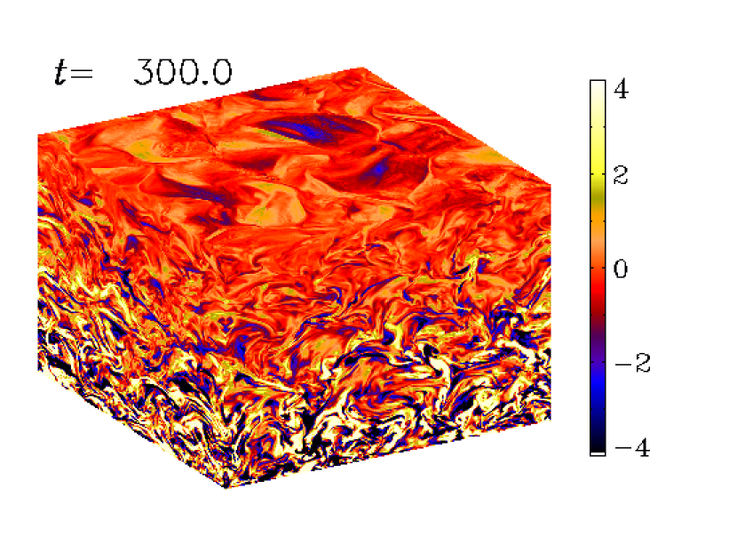
Figure 1.— Visualization of $\Delta B_{y}/B_{\rm eq}$ on the periphery of the computational domain for Model U1h600 with $B_{0}/B_{\rm eq0}=0.1$ at $\mbox{\rm Re}_{M}\approx 600$ using $512^{3}$ meshpoints.

Table 1 Summary of all DNS models discussed in this paper.

Model $\mbox{\rm Re}_{M}$ $\mbox{\rm Pr}_{M}$ $\beta_{0}$ $q_{p0}$ $\beta_{\star}$ $\beta_{\rm rms}$ Res. U1h05 0.5 0.5 0.1 0.2 0.32 *0.04 $64^{2}\times 128$ U1h1 1.5 0.5 0.1 0.2 0.32 *0.08 $64^{2}\times 128$ U1h5 5 0.5 0.1 4 0.34 *0.15 $64^{2}\times 128$ U1h10 10 0.5 0.1 13 0.33 *0.20 $128^{3}$ U1h20 23 0.5 0.1 40 0.33 *0.29 $128^{3}$ U1o35 35 1 0.1 90 0.35 *0.40 $128^{3}$ U1t35 35 2 0.1 70 0.34 *0.44 $128^{3}$ U1f35 35 4 0.1 15 0.28 *0.44 $128^{3}$ U1e35 35 8 0.1 0.2 0.32 *0.38 $128^{3}$ U1h40 42 0.5 0.1 170 0.38 *0.82 $128^{3}$ U1q70 70 1/4 0.1 250 0.37 0.14 $128^{3}$ U1h70 70 0.5 0.1 100 0.33 0.31 ${\bf 128^{3}}$ U1h70h 70 0.5 0.1 60 0.30 0.29 $256^{3}$ U1o70 70 1 0.1 50 0.29 0.42 $128^{3}$ U1t70 70 2 0.1 50 0.26 0.49 $128^{3}$ U1f70 70 4 0.1 20 0.22 0.55 $128^{3}$ U1e70 70 8 0.1 – – 0.49 $128^{3}$ U2h70 70 0.5 0.2 130 0.35 0.31 $128^{3}$ U5h70 70 0.5 0.5 200 0.39 0.31 $128^{3}$ U1a140 140 1/8 0.1 200 0.31 0.43 $256^{3}$ U1q140 140 1/4 0.1 40 0.27 0.49 $128^{3}$ U1h140 140 0.5 0.1 50 0.27 0.53 $128^{3}$ U1h250 250 0.5 0.1 40 0.20 0.68 $256^{3}$ U1h600 600 0.5 0.1 40 0.22 0.82 $512^{3}$ B07h35 35 0.5 0.07 – – *0.15 $128^{3}$ B2h35 35 0.5 0.2 – – *0.30 $128^{3}$

We have computed $q_{p}$ for all models of type U. We plot in Fig. 2 the dependence of $q_{p}$ on height for three different values of $B_{0}$. In the following, the case with $B_{0}/B_{\rm eq0}=0.1$ will be used as our fiducial run. To improve the statistics, we present here time averaged results of $q_{p}$, which itself is already averaged over $x$ and $y$. Error bars have been calculated by dividing the time series into three equally long pieces and computing the maximum departure from the total average. In agreement with earlier work, $q_{p}$ is always positive and exceeds unity when the mean magnetic field is not sufficiently strong. This is the case primarily at the bottom of the domain (negative values of $z$) where the density is high and therefore the magnetic field, in units of the equipartition field strength, is weak. Since $B_{0}={\rm const}{}$ and $B_{\rm eq}$ increases with depth, $B_{0}/B_{\rm eq}$ is smallest at the bottom, so $q_{p}$ also increases. The sharp uprise toward the lower boundary is just a result of the exponential increase of the density combined with the fact that the horizontal velocity reaches a local maximum on the boundary.

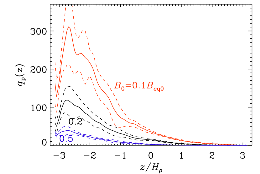
Figure 2.— Dependence of $q_{p}(z)$ (solid lines) with error margins (dashed lines) as functions of $z$, for Models U1h70, U2h70, and U5h70 with $B_{0}=0.1B_{\rm eq0}$, $B_{0}=0.2B_{\rm eq0}$, and $B_{0}=0.5B_{\rm eq0}$, with $\mbox{\rm Re}_{M}\approx 70$, $g/c_{s}^{2}k_{1}=1$, and a density contrast of 530. Note that $q_{p}(z)$ reaches a maximum at the bottom of the domain where $B_{0}/B_{\rm eq}(z)$ is minimal.

The total effective magnetic pressure of the mean field (that takes into account the effects of turbulence on the mean Lorentz force) is given by ${\textstyle{1\over 2}}[1-q_{p}(\overline{B})]\overline{\mbox{\boldmath$B$}}{}^{2}$. This has to be compared with the turbulent kinetic energy density, ${\textstyle{1\over 2}}\overline{\rho\mbox{\boldmath$u$}{}^{2}}$. Small contributions of terms $\propto q_{g}$ to the effective mean magnetic pressure are discussed in Sect. 3.3. In Fig. 3 we plot the effective magnetic pressure normalized by $B_{\rm eq}^{2}$,

$${\cal P}_{\rm eff}={\textstyle{1\over 2}}(1-q_{p})\overline{\mbox{\boldmath$B$}}{}^{2}/B_{\rm eq}^{2},$$ (18)

where $B_{\rm eq}^{2}$ itself is a function of height; see Eq. (8). It turns out that this function now reaches a negative minimum somewhere in the middle of the domain. Work of Kemel et al. (2012b) has shown that the regions below the minimum value of ${\cal P}_{\rm eff}$ are those that can potentially display NEMPI.

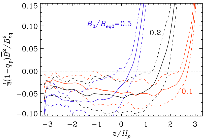
Figure 3.— Normalized effective mean magnetic pressure as a function of depth for the same models as in Fig. 2. Note that this function now reaches a negative minimum somewhere in the middle of the domain.

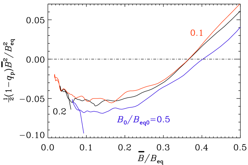
Figure 4.— Same as Fig. 3, but as a parametric representation as function of the local value of the ratio $B_{0}/B_{\rm eq}(z)$. Note that the curves for $B_{0}=0.1B_{\rm eq0}$, $B_{0}=0.2B_{\rm eq0}$, and $B_{0}=0.5B_{\rm eq0}$ collapse onto a single dependency. The error range is the same as in the previous figure, but not shown for clarity.

Figure 5.— Dependence of the fit parameters on $\mbox{\rm Re}_{M}$ using Models U1h05–U1h600.

We expect that $q_{p}$ is a function of the ratio of $\overline{B}/B_{\rm eq}$. This was observed numerically in BKR for constant $B_{\rm eq}$ by varying the value of $B_{0}$ to obtain $q_{p}$ for a range of different simulations. In the present case, however, $B_{\rm eq}$ is a function of $z$, which is the main reason why $q_{p}$ depends on height. In Fig. 4 we plot the effective mean magnetic pressure as a function of magnetic field in units of the local equipartition value. Note that now all three curves for different values of $\overline{B}$ collapse onto a single curve, which demonstrates that the dependence of $q_{p}$ on both $\overline{B}$ and $z$ can indeed be reduced to a single dependence on the ratio $\beta=|\overline{\mbox{\boldmath$B$}}{}|/B_{\rm eq}(z)$.

To quantify the form of the $q_{p}(\beta)$ dependence, we used in BKR a fit formula involving an arctan function. However, following recent work of Kemel et al. (2012b), a sufficient and certainly much simpler fit formula is

$$q_{p}(\beta)={q_{p0}\over 1+\beta^{2}/\beta_{p}^{2}}.$$ (19)

Here the fit parameters $q_{p0}$ and $\beta_{p}$ are determined by measuring the minimum effective magnetic pressure, ${\cal P}_{\rm min}=\min({\cal P}_{\rm eff})$, as well as the position of the minimum, $B_{\rm min}$, where ${\cal P}_{\rm eff}(B_{\rm min})={\cal P}_{\rm min}$. For our setups, ${\cal P}_{\rm min}$ is typically around $-0.05$, while $\beta_{\rm min}=B_{\rm min}/B_{\rm eq}$ is between 0.1 and 0.2. This is remarkably close to Fig. 3 of RK07, who used the spectral $\tau$ relaxation approximation. The fact that nearly the same functional form for the effective magnetic pressure of the mean field is obtained, supports the idea that this effect is robust.

For many of the models in Table LABEL:ModelsU we have determined the fit parameters $q_{p0}$ and $\beta_{p}$. It turns out that for small values of $\mbox{\rm Re}_{M}$, $q_{p0}$ increases quadratically with $\mbox{\rm Re}_{M}$ and $\beta_{p}$ decrease like $\mbox{\rm Re}_{M}^{-1}$. Thus, for $\mbox{\rm Re}_{M}<30$, we have $\beta_{\star}^{2}\equiv\beta_{p}^{2}q_{p0}\approx{\rm const}{}$. The significance of this is that $\beta_{\star}$ turns out to be nearly independent of $\mbox{\rm Re}_{M}$; see Fig. 5. It allows rewriting the fit formula as

$$q_{p}(\beta)={\beta_{*}^{2}\over\beta_{p}^{2}+\beta^{2}},$$ (20)

where for small values of $\mbox{\rm Re}_{M}$, only $\beta_{p}$ depends on $\mbox{\rm Re}_{M}$. In particular, we have then $\beta_{p}\approx 1.05/\mbox{\rm Re}_{M}$.

The obtained scaling for $q_{p0}\sim 0.1\mbox{\rm Re}_{M}^{2}$ is consistent with an estimate based on the quasi-linear calculations. This analysis is similar to that of Rüdiger et al. (2012), except that we performed an explicit integration in $\omega{\bm{k}}$-space for a power-law kinetic energy spectrum of the background turbulence and for a Lorentz profile for the frequency dependence of the velocity correlation function. For $\beta\ll 1$ this analysis yields the expression (see Appendix A)

$$q_{p0}={8-\mbox{\rm Pr}_{M}\over 60\,\mbox{\rm Pr}_{M}}\mbox{\rm Re}_{M}^{2},$$ (21)

where $\mbox{\rm Re}_{M}^{2}/\mbox{\rm Pr}_{M}=\mbox{\rm Re}_{M}\mbox{\rm Re}$. For $\mbox{\rm Pr}_{M}=1/2$, we have $q_{p}=0.25\,\mbox{\rm Re}_{M}^{2}$, which is in qualitative agreement with our scaling for $q_{p0}$. The discrepancy in the coefficient is related to the fact that the quasi-linear approach is only valid for small magnetic and fluid Reynolds numbers. Therefore, the limit $\mbox{\rm Pr}_{M}\to 0$ in the framework of the quasi-linear approach only implies the case of large magnetic diffusion $\eta$, while the case of small $\nu$ need to be considered in the framework of approaches that are valid for large fluid Reynolds numbers (like the $\tau$ relaxation approach).

Looking at Table LABEL:ModelsU, it may seem surprising that $q_{p0}$ can reach values as large as 250 (see, e.g., Model U1q70 with $\mbox{\rm Re}_{M}\approx 250$ and $\mbox{\rm Pr}_{M}=4$). However, the more relevant quantity is $q_{p}(\beta)\beta^{2}$, which is of the order of $\beta_{*}^{2}$ for large field strengths. Summarizing the results from Fig. 5, we find

$$\beta_{p}\approx 1.05\,\mbox{\rm Re}_{M}^{-1},\quad\beta_{\star}=0.33\quad\mbox{(for $\mbox{\rm Re}_{M}<30$)},$$ (22)

and

$$\beta_{p}\approx 0.035,\quad\beta_{\star}=0.23\quad\mbox{(for $\mbox{\rm Re}_{M}>60$)},$$ (23)

which implies that $q_{p}(\beta)\beta^{2}$ is below 0.1 and 0.06 for the regimes applicable to Eqs. (22) and (23), respectively. Also, it is tempting to associate the sudden drop of $\beta_{\star}$ from 0.33 to 0.23 with the onset of small-scale dynamo action. The fact that small-scale dynamo action reduces the negative effect of turbulence on the effective mean magnetic pressure was already predicted by RK07 and is also quite evident by looking at Table LABEL:ModelsU, where $q_{p0}$ is found to reach more moderate values after having reached a peak at $\mbox{\rm Re}_{M}\approx 30$.

We reiterate that, as long as the value of the plasma beta (i.e. the ratio of gas pressure to magnetic pressure), is much larger than unity, our results are independent of the plasma beta. What matters is the ratio of magnetic energy density to kinetic energy density, not the thermal energy density. This is also clear from the equations given in Appendix B. In the present simulations, the plasma beta varies from between 5 and 100 at the top to around $10^{5}$ at the bottom, so the total pressure (gas plus magnetic plus turbulent pressure) is always positive.

3.2. Dependence on magnetic Prandtl number

In most of the runs discussed above we used $\mbox{\rm Pr}_{M}=1/2$. As expected from earlier work of RK07, the negative magnetic pressure effect should be most pronounced at small $\mbox{\rm Pr}_{M}$. This is indeed confirmed by comparing with larger and smaller values of $\mbox{\rm Pr}_{M}$; see Fig. 6, where we show the results for Models U1q70, U1h70, U1t70, and U1e70. Here and in Table LABEL:ModelsU the different values of $\mbox{\rm Pr}_{M}$ are denoted by the letters q, h, o, t, f, and e, which stand for a quarter, half, one, two, four, and eight, while the letter a is used for one eighth.

Figure 6.— Normalized effective mean magnetic pressure for different values of $\mbox{\rm Pr}_{M}$, for Models U1q70, U1h70, U1t70, and U1e70, where $\mbox{\rm Re}_{M}\approx 70$ and $B_{0}=0.1B_{\rm eq0}$.

3.3. Resolution dependence

A density contrast of over 500 may seem rather large. However, this impression may derive from experience with polytropic models (see, e.g., Cattaneo et al., 1991), where most of the density variation occurs near the surface. In our isothermal model, the scale height is constant, so the logarithmic density change is independent of height. Figure 7 shows that the error bars for the $256^{3}$ run are smaller than those for the $128^{3}$ run, and that the minimum of ${\cal P}_{\rm eff}$ is somewhat less shallow, but within error bars the two curves are still comparable. Here, the relevant input data are averaged over a time interval $\Delta t$ such that $u_{\rm rms}k_{f}\Delta t$ is at least 1500, and that error bars, which are based on 1/3 of that, cover thus at least 500 turnover times.

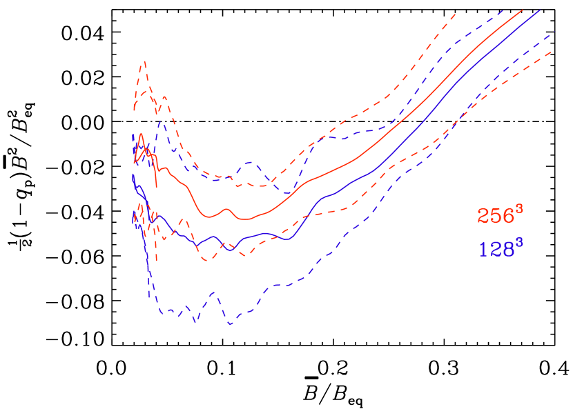
Figure 7.— Resolution dependence of $q_{p}(\overline{B}_{y}/B_{\rm eq})$ for $\mbox{\rm Pr}_{M}=1/2$, $\mbox{\rm Re}_{M}\approx 70$ for Models U1h70 and U1h70h using $128^{3}$ and $256^{3}$ mesh points. Error bars are marked by the dashed lines.

3.4. Coefficients $q_{s}$ and $q_{g}$

Depending on the size and magnitude of the coefficients $q_{s}$ and $q_{g}$, their effect on the instability could be significant. Most importantly, a positive value of $q_{s}$ was found to be chiefly responsible for producing three-dimensional mean-field structures (Kemel et al., 2012b), i.e., structures that break up in the direction of the imposed field. The coefficient $q_{g}$, on the other hand, affects the negative effective magnetic pressure and could potentially enhance its effect significantly (RK07).

Using Eqs. (15), we now determine $q_{s}$ and $q_{g}$. The results are shown in Figs. 8 and 9 for the three imposed field strengths considered above, where $\overline{\mbox{\boldmath$u$}{}^{2}}$ is nearly independent of $z$, so $B_{\rm eq}(z)$ varies by a factor of $\exp\pi\approx 23$, allowing us to scan the dependence on $\overline{B}/B_{\rm eq}$ in a single run. It turns out that both $q_{s}$ and $q_{g}$ are around zero.

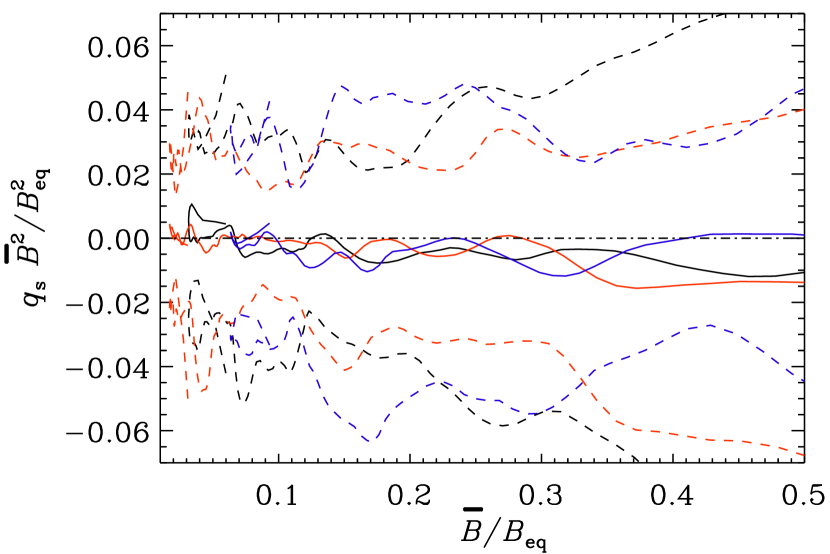
Figure 8.— Similar to Fig. 4, but for $q_{s}\overline{\mbox{\boldmath$B$}}{}^{2}/B_{\rm eq}^{2}$ and now as a function of $\overline{B}_{y}/B_{\rm eq}$. Within the error range (dashed lines), $q_{s}=0$ for all field strengths.

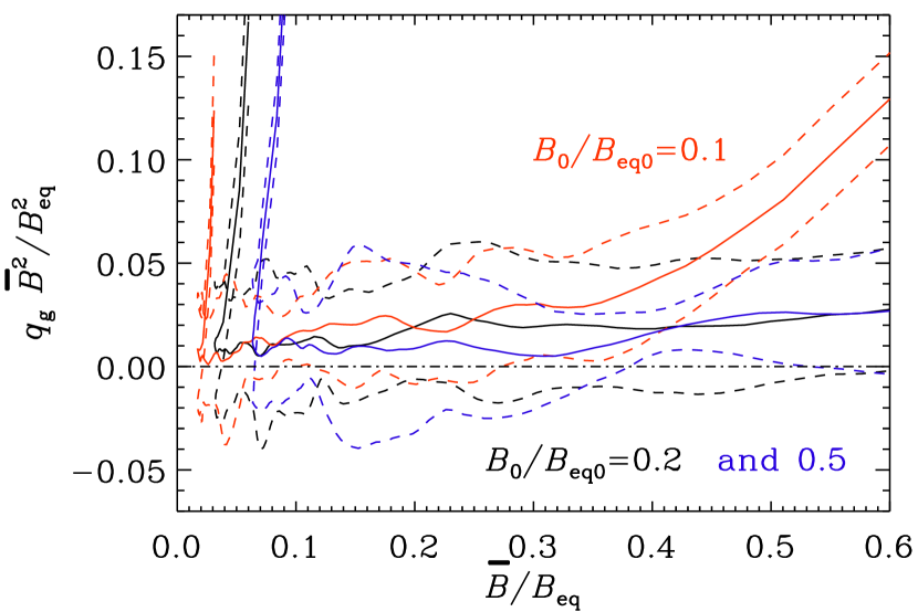
Figure 9.— Similar to Fig. 8, but for $q_{g}$. Note that $q_{g}$ is positive.

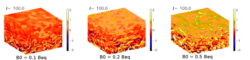
Figure 10.— Visualization of $\Delta B_{y}/B_{\rm eq}$ on the periphery of the computational domain for runs with $B_{0}/B_{\rm eq0}=0.1$, 0.2, and 0.5, with $\mbox{\rm Re}=70$.

Recent DNS of stratified convection with an imposed horizontal magnetic field did actually yield non-vanishing (positive) values of $q_{g}$ for stratified convection (Käpylä et al., 2012). In the present study with vertical density stratification, $q_{g}$ is much smaller, but generally positive. This appears to be in conflict with the theoretical expectation for $q_{g}$ given in Appendix B, where $q_{g}=O(\ell_{f}^{2}/H_{\rho}^{2})$ if we assume $\ell_{f}=2\pi/k_{f}\approx 1.3$, which gives $q_{g}\approx 1.2$. However, without the $2\pi$ factor, we would have $\ell_{f}=k_{f}^{-1}=0.2$, and thus $q_{g}\approx-0.03$. Fig. 9 suggests a positive value of similar magnitude. This issue will hopefully be clarified soon in future work.

Next, we discuss the results for $q_{s}$. In BKR there was some evidence that $q_{s}$ can become positive in a narrow range of field strengths, but the error bars were rather large. The present results are more accurate and suggest that $q_{s}\overline{\mbox{\boldmath$B$}}{}^{2}/B_{\rm eq}^{2}$ is essentially zero. This is also in agreement with recent convection simulations (Käpylä et al., 2012).

In summary, the present simulations provide no evidence that the coefficients $q_{s}$ and $q_{g}$ could contribute to the large-scale instability that causes the magnetic flux concentrations. This is not borne out by the analytic results given in Appendix B. The results from recent convection simulations fall in between the analytic and numerical results mentioned above, because in those $q_{g}$ was found to be positive, while $q_{s}$ was still found to be small and negative (Käpylä et al., 2012).

4. Comparison of models of types U and B

4.1. Results from DNS

As discussed in the beginning of Sect. 3.1, most of the variability of the magnetic field occurs near the bottom of the computational domain. This is also evident from Fig. 10, where we show visualizations of the $y$ component of the departure from the imposed field, $\Delta B_{y}$, on the periphery of the domain for Models U1h70, U2h70, and U5h70 with $B_{0}/B_{\rm eq0}=0.1$, 0.2, and 0.5, respectively.

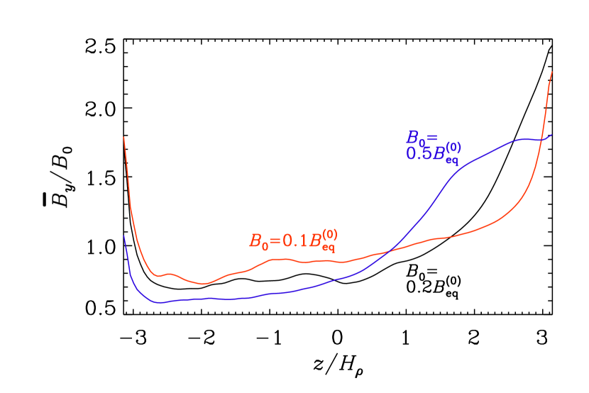
Figure 11.— Normalized mean magnetic field in the direction of the imposed field versus height for $B_{0}=0.1B_{\rm eq0}$, $0.2B_{\rm eq0}$, and $0.5B_{\rm eq0}$ with $\mbox{\rm Re}=70$.

The vertical dependence of the horizontally averaged mean magnetic field (now normalized to $B_{0}={\rm const}{}$) is shown in Fig. 11. We see that, especially for intermediate field strengths, there is an increase of the magnetic field near the top of the domain. One possibility is that this is caused by the effect of nonlinear turbulent pumping, which might cause the mean field to be pumped up due to the gradients of the mean turbulent kinetic energy density in the presence of a finite mean magnetic field (cf. Rogachevskii & Kleeorin, 2006). This type of pumping is different from the regular pumping down the gradient of turbulent intensity (Rädler, 1969). To eliminate this effect, we have produced additional runs where the kinetic energy density is approximately constant with height. This is achieved by modulating the forcing function by a $z$-dependent factor $e^{z/H_{\it f}}$. We define $n=H_{\it f}/H_{\rho}$ and find that for $n=1.4$ the kinetic energy density is approximately independent of height; see Fig. 12.

Figure 12.— Turbulent kinetic energy density versus height for $n=\infty$ for $B_{0}=0$ (dotted line) and $B_{0}=0.2B_{\rm eq0}$ compared with the case for $n=1.4$ and $B_{0}=0.2B_{\rm eq0}$.

As a consequence of reducing the turbulent driving in the lower parts by having $B_{\rm eq}(z)\approx{\rm const}{}$, we allow the magnetic field to have almost the same energy density as the turbulence, i.e. $B_{0}/B_{\rm eq}(z)$ is approximately independent of $z$. This also means that the fluctuations are now no longer so pronounced at the bottom of the domain (Fig. 13), where Re drops to values around 5 and the flow is no longer turbulent. However, at the top the Reynolds number is around 120, so here the flow is still turbulent. In Fig. 14 we show the vertical dependence of the horizontally averaged mean magnetic field in units of the imposed field strength. Note that now the field shows an increase toward the bottom of the domain. This effect might be related to regular turbulent pumping (Rädler, 1969), which now has a downward component because $\overline{\mbox{\boldmath$u$}{}^{2}}$ decreases with depth.

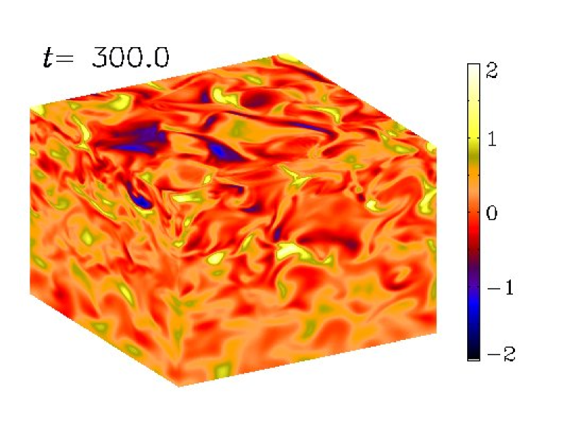
Figure 13.— Visualization of $\Delta B_{y}/B_{\rm eq}$ on the periphery of the computational domain for Model B1h35 with nearly uniform turbulent kinetic energy density using $H_{\it f}=nH_{\rho}$ with $n=1.4$.

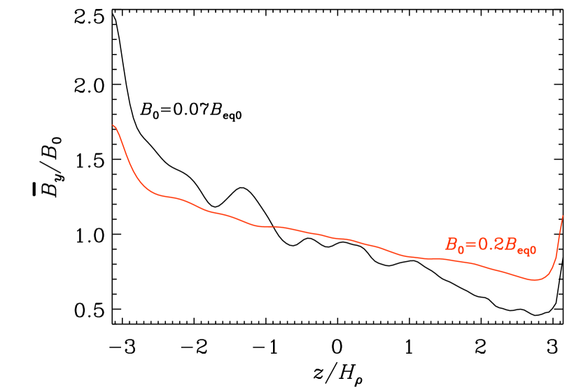
Figure 14.— Normalized mean magnetic field in the direction of the imposed field versus height in the case of nearly constant turbulent kinetic energy density, i.e. $B_{\rm eq}(z)\approx{\rm const}{}$, for Models B07h35 and B2h35 with $B_{0}/B_{\rm eq0}=0.07$ and 0.2, respectively.

4.2. Determination of $\eta_{t}$ and $\gamma$ from the simulations

We use the test-field method of Schrinner et al. (2005, 2007) in the Cartesian implementation, as described by Brandenburg et al. (2008a), to compute $\eta_{t}$ and $\gamma$ from the simulations in the presence of the applied field. We refer to this as the quasi-kinematic test-field method, which is applicable if the magnetic fluctuations are just a consequence of the mean field; see Rheinhardt & Brandenburg (2010) for details and extensions to a fully nonlinear test-field method. For further comments regarding the test-field method see Appendix C. We analyze the two setups discussed above, namely those of type U (where $u_{\rm rms}$ and hence $\eta_{t}$ are nearly constant in height) and those of type B (where $B_{\rm eq}$ is nearly constant in height).

The set of test fields includes constant and linearly growing ones. For both models we use $B_{0}=0.01\rho^{1/2}c_{s}$, corresponding to $B_{0}\approx 0.1B_{\rm eq0}$ for models of type U and $B_{0}\approx 0.07B_{\rm eq0}$ for model of type B. The results are shown in Figs. 15 and 16 for Models B07h35 and U1h70, respectively. In Table LABEL:Tsummary we summarize the relevant parameters inferred for these models. It turns out that the DNS results are well described by $\eta_{t}=1.2\,\eta_{t0}$, with $\eta_{t0}=u_{\rm rms}/3k_{f}$ and $u_{\rm rms}(z)=u_{\rm rms0}\exp(z/H_{u})$, but $\gamma=-{\rm d}{}\eta_{t}/{\rm d}{}z$, i.e. without the 1/2 factor expected from the kinematic mean-field theory (Rädler, 1969).

Figure 15.— Results for $\eta_{t}$ and $\gamma$ with the test-field method (solid lines; error margins are shown as dashed lines) for Model B07h35. In the upper panel, the dotted line gives $1.2\,u_{\rm rms}/3k_{f}$ and the dash-dotted line represents $1.2\,u_{\rm rms0}\exp(z/H_{u})/3k_{f}$. In the lower panel, the dash-dotted lines represents $-1.2\,u_{\rm rms0}\exp(z/H_{u})/3k_{f}H_{u}$.

Figure 16.— Same as Fig. 15, but for Model U1h70.

We emphasize that $\mbox{\boldmath$\gamma$}{}\approx\bm{0}$ for models of type U, suggesting that additional effects owing to the mean magnetic field such as mean-field magnetic buoyancy (Kitchatinov et al., 1994; Rogachevskii & Kleeorin, 2006) are weak (Appendix D).

4.3. Comparison with mean-field models

4.3.1 Basic equations

We follow here the same procedure as BKR and consider the equations for the mean velocity $\overline{\bm{U}}$, the mean density $\overline{\rho}$, and the mean vector potential $\overline{\mbox{\boldmath$A$}}{}$ in the form

$${\partial\overline{\bm{U}}\over\partial t}=-\overline{\bm{U}}\cdot\mbox{\boldmath$\nabla$}{}\overline{\bm{U}}-c_{s}^{2}\mbox{\boldmath$\nabla$}{}\ln\overline{\rho}+\mbox{\boldmath$g$}{}+\overline{\mbox{\boldmath${\cal F}$}}{}^{M}+\overline{\mbox{\boldmath${\cal F}$}}{}_{K,{\rm tot}},$$ (24)

$${\partial\overline{\mbox{\boldmath$A$}}{}\over\partial t}=\overline{\bm{U}}\times\overline{\mbox{\boldmath$B$}}{}+\overline{\mbox{\boldmath${\cal E}$}}{}-\eta\overline{\mbox{\boldmath$J$}}{}-\mbox{\boldmath$\nabla$}{}\overline{\Phi},$$ (25)

$${\partial\overline{\rho}\over\partial t}=-\mbox{\boldmath$\nabla$}{}\cdot\overline{\rho}\overline{\bm{U}},$$ (26)

where $\overline{\Phi}$ is the mean electrostatic potential, $\overline{\mbox{\boldmath$B$}}{}=\mbox{\boldmath$B$}{}_{0}+\mbox{\boldmath$\nabla$}{}\times\overline{\mbox{\boldmath$A$}}{}$ is the mean magnetic field including the imposed field, and

$$\overline{\rho}\overline{\mbox{\boldmath${\cal F}$}}{}^{M}=\overline{\mbox{\boldmath$J$}}{}\times\overline{\mbox{\boldmath$B$}}{}+{\textstyle{1\over 2}}\mbox{\boldmath$\nabla$}{}(q_{p}\overline{\mbox{\boldmath$B$}}{}^{2})$$ (27)

is the effective mean Lorentz force, where we use for $q_{p}(\overline{B})$ the fit formula given by Eq. (19). However, in view of the results of Sect. 3.4, the $q_{s}$ and $q_{g}$ terms will now be omitted, and

$$\overline{\mbox{\boldmath${\cal F}$}}{}_{K,{\rm tot}}=(\nu_{t}+\nu)\left(\nabla^{2}\overline{\bm{U}}+\mbox{\boldmath$\nabla$}{}\mbox{\boldmath$\nabla$}{}\cdot\overline{\bm{U}}+2\overline{\mbox{\boldmath${\mathsf{S}}$}}{}\mbox{\boldmath$\nabla$}{}\ln\overline{\rho}\right)$$ (28)

is the total (turbulent and microscopic) viscous force,

$$\overline{\mbox{\boldmath${\cal E}$}}{}=\mbox{\boldmath$\gamma$}{}\times\overline{\mbox{\boldmath$B$}}{}-\eta_{t}\overline{\mbox{\boldmath$J$}}{},$$ (29)

is the mean electromotive force, where $\gamma$ is the turbulent pumping velocity and $\eta_{t}$ is the turbulent magnetic diffusivity. In our mean-field models we assume $\nu_{t}/\eta_{t}=1$ (Yousef et al., 2003). The kinematic theory of Roberts & Soward (1975) and others predicts that $\eta_{t}(z)=u_{\rm rms}(z)/3k_{f}$ and $\mbox{\boldmath$\gamma$}{}=-{\textstyle{1\over 2}}\mbox{\boldmath$\nabla$}{}\eta_{t}$. It is fairly easy to assess the accuracy of these expressions by computing turbulent transport coefficients from the simulations using the test-field method (Schrinner et al., 2005, 2007).

A comment regarding $\overline{\Phi}$ is here in order. It is advantageous to isolate a diffusion operator of the form $\eta_{t}\nabla^{2}\overline{\mbox{\boldmath$A$}}{}$ by using the so-called resistive gauge in which $\overline{\Phi}=-\eta_{t}\mbox{\boldmath$\nabla$}{}\cdot\overline{\mbox{\boldmath$A$}}{}$. This means that the diffusion operator now becomes $\eta_{t}\nabla^{2}\overline{\mbox{\boldmath$A$}}{}+(\mbox{\boldmath$\nabla$}{}\cdot\overline{\mbox{\boldmath$A$}}{})\mbox{\boldmath$\nabla$}{}\eta_{t}$ (Dobler et al., 2002). This formulation is advantageous in situations in which $\eta_{t}$ is non-uniform.

4.3.2 Results from the mean-field models

Next we consider solutions of Eqs. (24)–(29) for models of types U and B using the parameters specified in Table LABEL:Tsummary. To distinguish these mean-field models from the DNS results, we denote them by script letters ${\cal U}$ and ${\cal B}$. We have either constant $\eta_{t}$ (Models ${\cal U}$) or constant $B_{\rm eq}$ (Models ${\cal B}$). In both cases we use $\eta=2\nu=4\times 10^{-4}c_{s}/k_{1}$, $B_{0}=0.005\rho^{1/2}c_{s}$, with $q_{p0}=40$ and $\beta_{p}=0.07$, while $B_{\rm eq0}$ and $\rho_{0}$ are given in Table LABEL:Tsummary and correspond to values used in the DNS. This gives the profile of $u_{\rm rms}(z)=B_{\rm eq}/\sqrt{\rho}$, which allows us to compute $\eta_{t}(z)=u_{\rm rms}(z)/3k_{f}$ and $\nu_{t}(z)=\eta_{t}(z)$ for an assumed value of $k_{f}$. In the DNS presented here we used $k_{f}/k_{1}=5$ and did not find evidence for NEMPI, but the DNS of Brandenburg et al. (2011) and Kemel et al. (2012a) for $k_{f}/k_{1}=15$ and $k_{f}/k_{1}=30$, respectively did show NEMPI, so we mainly consider the case $k_{f}/k_{1}=15$, but we also consider $k_{f}/k_{1}=5$ and 10.

As in BKR, Eqs. (24)–(26) exhibit a linear instability with subsequent saturation. However, this result is still remarkable because there are a number of differences compared with the models studied in BKR. Firstly, we consider here an isothermal atmosphere which is stably stratified, unlike the isentropic one used in BKR, which was only marginally stable. This underlines the robustness of this model and shows that this large-scale instability can be verified over a broad range of conditions. Secondly, this instability also works in situations where $\eta_{t}$ and/or $B_{\rm eq}$ are non-uniform and where there is a pumping effect that sometimes might have a tendency to suppress the instability.

Figure 17.— Evolution of the mean velocity for Models ${\cal U}$ and ${\cal B}$ obtained by solving the mean field equations. “Model ${\cal B}$0 ($\gamma=0$)” refers to a model where the pumping velocity is ignored. In all cases, $k_{f}/k_{1}=15$ is assumed. In the inset we compare the evolution for Model ${\cal U}$ with those for smaller values of $k_{f}/k_{1}$ (Model ${\cal U}$10 and ${\cal U}$5).

In Fig. 17 we compare the evolution of the rms velocity of the mean flow. Note that, in contrast to the corresponding plots in BKR, we have here normalized $\overline{U}_{\rm rms}$ with respect to $v_{A0}\equiv B_{0}/\sqrt{\rho_{0}}$ and time is normalized with respect to the Alfvén wave traveling time, $(v_{A0}k_{1})^{-1}$. This was done because in these units the curves for Models ${\cal U}$ and ${\cal B}$ show similar growth rates. This is especially true when the pumping term is ignored in Model ${\cal B}$0, where we have set artificially $\gamma=0$. With pumping included (as was determined from the kinematic test-field method), the growth rate is slightly smaller (compare dashed and dotted lines). The pumping effect does not significantly affect the nonlinear saturation phase, i.e. the late-time saturation behavior for the two versions of Model ${\cal B}$ is similar. Instead, the saturation phase is different for Model ${\cal U}$ compared with Model ${\cal B}$ and the saturation value is larger for Model ${\cal U}$. The inset of Fig. 17 compares the results for Model ${\cal U}$ (with $k_{f}/k_{1}=15$) with Models ${\cal U}$10 and ${\cal U}$5 for $k_{f}/k_{1}=10$ and 5, respectively. Note that NEMPI is quite weak for $k_{f}/k_{1}=5$, which is consistent with the DNS presented here.

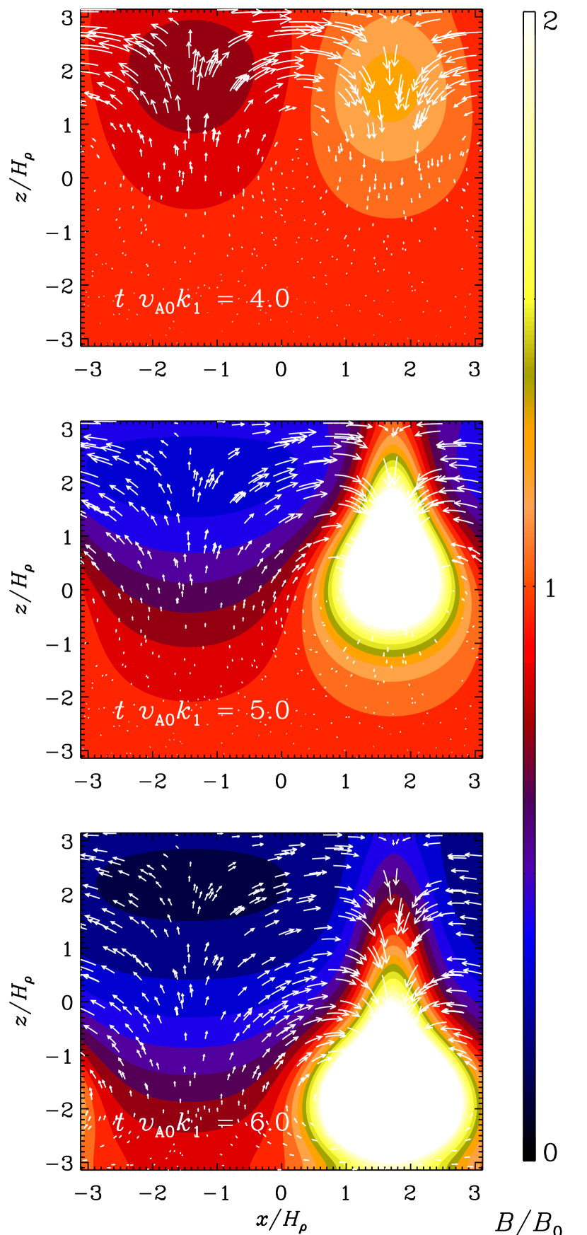
Figure 18.— Mean magnetic field in the $y$ direction (color coded) together with velocity vectors in the $xz$ plane for Model ${\cal U}$02. Note the spontaneous formation of flux structures.

Visualizations of the mean magnetic field as well as the mean velocity are shown in Fig. 18 for three different times near saturation for Model ${\cal U}$02. Here, we use a weaker imposed field, $B_{0}=0.002\rho^{1/2}c_{s}$, corresponding to $B_{0}/B_{\rm eq0}=0.02$, so that NEMPI starts closer to the surface. For $B_{0}/B_{\rm eq0}=0.05$, NEMPI starts in the middle of the domain, leaving less space before the structures have reached the bottom of the domain. Note the converging flows toward the magnetic structures, with the largest velocities occurring in the upper layers where the density is smallest.

Table 2 Summary of parameters entering models U and B.

Model $\tilde{k}_{f}$ $\tilde{\eta}_{t0}$ $\tilde{B}_{\rm eq0}$ $\beta_{0}$ $\mbox{\rm Re}_{M}$ comment ${\cal U}$ 15 0.0072 0.11 0.05 36 $B_{\rm eq}=B_{\rm eq0}\,e^{-z/2H_{\rho}}$ ${\cal U}$10 10 0.0048 0.11 0.05 36 $B_{\rm eq}=B_{\rm eq0}\,e^{-z/2H_{\rho}}$ ${\cal U}$5 5 0.0024 0.11 0.05 36 $B_{\rm eq}=B_{\rm eq0}\,e^{-z/2H_{\rho}}$ ${\cal U}$02 15 0.0072 0.11 0.02 36 $B_{\rm eq}=B_{\rm eq0}\,e^{-z/2H_{\rho}}$ ${\cal B}$ 15 0.0024 0.036 0.05 2.5–60 $\eta_{t}=\eta_{t0}\,e^{z/2H_{\rho}}$ ${\cal B}$0 15 0.0024 0.036 0.05 2.5–60 $\gamma=0$ assumed

4.3.3 Comments on the shape of mean-field structures

The descending structures found in the present mean-field calculations are qualitatively similar to those of BKR who considered a polytropic layer. In both cases the structures sink and become wider. This is quite different from the behavior of individual turbulent eddies and flux tubes that one tends to monitor in DNS. Clearly, individual magnetic structures experience magnetic buoyancy, where the vertical motion is the result of a balance of magnetic buoyancy and downward advection by the ambient flow (see Fig. 10 of Brandenburg et al., 1996). The mean-field model cannot describe individual (small-scale) structures, although the net effect of the vertical motion of individual structures results in a turbulent pumping velocity $\gamma$ of mean-field structures.

While turbulent downward pumping has been seen in numerous DNS, the negative effective magnetic pressure instability is a new effect that has been seen so far only in the DNS of forced turbulence in BKKMR; see also Kemel et al. (2012a). Amazingly, those DNS show very similar structures resembling that of a descending “potato sack” (see Fig. 1 of BKKMR). They sink because the negative effective magnetic pressure is compensated by increased gas pressure, which in turn leads to larger density, so they become heavier than the surroundings. However, these turbulent magnetic structures are only poorly associated with material motion; see the flow vectors in Fig. 18. Therefore, a change of their volume is not governed by mass conservation. In particular, these structures do not become narrower during their descent as individual blobs do in a strongly stratified layer.

We should point out that these mean-field structures do not always initiate at the top of the layer. The initiation height depends on the value of $z$ where ${\cal P}_{\rm eff}$ reaches a minimum. Larger values of $B_{0}$ tend to move this location downward; see Fig. 2. A more detailed exploration of this is given by Kemel et al. (2012b).

4.3.4 Comparison with the Parker instability

NEMPI can be understood as a generalization of the Parker instability. This becomes evident when considering the stability criterion of NEMPI (RK07):

$$(H_{\rho}-H_{B})\left.{{\rm d}{}{\cal P}_{\rm eff}\over{\rm d}{}\beta^{2}}\right|_{\beta_{0}}>0,$$ (30)

where ${\rm d}{}{\cal P}_{\rm eff}/{\rm d}{}\beta^{2}={\textstyle{1\over 2}}(1-q_{p}-{\rm d}{}q_{p}/{\rm d}{}\ln\beta^{2})$ and $H_{B}$ is the characteristic spatial scale of the mean magnetic field variations. However, unlike the Parker instability, NEMPI can be excited even in a uniform mean magnetic field ($H_{B}\to\infty$). The source of free energy of this instability is provided by the small-scale turbulent fluctuations. In contrast, the free energy in the Parker’s magnetic buoyancy instability (Parker, 1966) or in the interchange instability in plasma (Tserkovnikov, 1960) is drawn from the gravitational field. In the absence of turbulence ($q_{p}=0$), condition (30) coincides with the criterion for the Parker’s magnetic buoyancy instability ($H_{\rho}>H_{B}$).

5. Conclusions

Our DNS have shown that for an isothermal atmosphere with strong density stratification the total turbulent pressure is decreased due to the generation of magnetic fluctuations by the tangling of an imposed horizontal mean magnetic field by the velocity fluctuations. This phenomenon strongly affects the mean Lorentz force so that the effective mean magnetic pressure becomes negative. For our numerical model with approximately uniform turbulent rms velocity, the ratio of imposed to equipartition field strength changes with height, because the density decreases with height, while the imposed field is constant. This allows us to determine the full functional form of the effective mean magnetic pressure as a function of normalized field strength for a single run.

The form of the dependence of ${\cal P}_{\rm eff}(\overline{B}/B_{\rm eq})$ is similar to that found for simulations under rather different conditions (with or without stratification, with or without convection, etc). This dependence is found to be similar to that obtained earlier using both analytic theory (RK07) and direct numerical simulations (BKR), and the results are robust when changing the strength of the imposed field.

In simulations where the turbulent velocity is nearly independent of height, the reduction of magnetic fluctuations occurs in the upper layers where the equipartition field strength decreases with height (models of type U). In models of type B, where the equipartition field strength is nearly constant in height, the magnetic fluctuations are found to be slightly stronger in the upper parts.

In view of astrophysical applications, it is encouraging that $q_{p0}$ and $\beta_{p}$ seem to approach an asymptotic regime for $\mbox{\rm Re}_{M}>60$. While it remains important to confirm this result, a number of other aspects need to be clarified. Firstly, the issue of finite scale separation is important, i.e., the larger the wavenumber of structures in the mean field relative to $k_{f}$, the less efficient the negative effective magnetic pressure will be. This needs to be quantified. For example in the work of Brandenburg et al. (2011), where we had a scale separation ratio of 1:15, magnetic structures were best seen after averaging along the direction of the mean field. On the other hand, with a scale separation ratio of 1:30, structures where quite pronounced already without averaging (Kemel et al., 2012a). In the Sun, the scale separation ratio is very large in the horizontal direction, but in the vertical direction the system is extremely inhomogeneous and the vertical pressure scale height increases rapidly with depth. The significance of such effects on the negative effective magnetic pressure effect remains still quite unclear.

Another aspect concerns the limitations imposed by the use of an isothermal equation of state. In the context of regular (non-turbulent) magnetic buoyancy, the system is known to be more unstable to the buoyancy instability when the fluctuations evolve isothermally (Acheson, 1978; Hughes & Weiss, 1995; MacGregor & Cassinelli, 2003). However, in the context of the negative effective magnetic pressure instability it is not clear in which direction this effect would work. The only simulations where the equation for specific entropy was taken into account are the simulations of Käpylä et al. (2012), who also considered an unstably stratified atmosphere. In their case, the negative effective magnetic pressure was found to be greatly enhanced (deeper minimum of ${\cal P}_{\rm eff}$ and larger values of $B_{\rm min}$). Again, this is a subject that deserves serious attention.

The fact that the values of $q_{p0}$ and $\beta_{p}$ appear to be converged in the range $60<\mbox{\rm Re}_{M}<600$ is significant, because this is also the regime in which small-scale dynamo action occurs. Small-scale dynamo action suppresses the magnetic pressure effect, which is the reason for the drop of $q_{p0}$ between $\mbox{\rm Re}_{M}$ of 40 and 60, but for larger $\mbox{\rm Re}_{M}$, the values of $q_{p0}$ seem roughly unchanged.

In the present paper we have discussed applications mainly to the Sun. However, any hydromagnetic turbulence with strong stratification and large plasma beta should be subject to the negative effective magnetic pressure phenomenon. Another relevant example might be accretion disks. Quasi-periodic oscillations and other light curve variations from accretion disks have long been suspected to be caused by some kind of structures in these disks. Hydrodynamic vortices would be one possibility (Abramowicz et al., 1992), which could constitute long-lived structures (Barge & Sommeria, 1995; Johansen et al., 2004; Lyra et al., 2011). However, in view of the present results, structures caused by the negative effective magnetic pressure instability might indeed be another candidate.

Appendix A Derivation of Equation (21)

We use the quasi-linear approach or second order correlation approximation applied to a random flow with small magnetic and fluid Reynolds numbers (e.g. Moffatt, 1978; Krause & Rädler, 1980; Rüdiger et al., 2012). We eliminate the pressure term from the equation for the velocity fluctuations ${\bm{u}}$ by calculating $\mbox{\boldmath$\nabla$}{}{\bm{\times}}(\mbox{\boldmath$\nabla$}{}{\bm{\times}}{\bm{u}})$, rewrite the obtained equation and the induction equation for the magnetic fluctuations ${\bm{b}}$ in Fourier space, apply the two-scale approach (Roberts & Soward, 1975), and neglect nonlinear terms, but retain molecular dissipative terms. This allows us to get the following equation for $\Delta\overline{\Pi}_{ij}^{f}$ from Eq. (9) in Fourier space:

$$\Delta\overline{\Pi}_{ij}^{f}({\bm{k}},\omega)=-\left[\hat{L}\left(1+{G_{\eta}^{\ast}(k,\omega)\over G_{\nu}(k,\omega)}\right)+\hat{L}^{\ast}\right]\overline{\Pi}_{ij}^{f,0}({\bm{k}},\omega),$$ (A1)

where $G_{\nu}(k,\omega)=(\nu k^{2}+i\omega)^{-1}$, $G_{\eta}(k,\omega)=(\eta k^{2}+i\omega)^{-1}$, $\hat{L}=G_{\nu}G_{\eta}k_{m}k_{n}\overline{B}_{m}\overline{B}_{n}$, and the background turbulence (with a zero mean magnetic field) is given by

$$\overline{\Pi}_{ij}^{f,0}({\bm{k}},\omega)={E(k)\,\Phi(\omega)\over 8\pi\,k^{2}}\,\Big{(}\delta_{ij}-{k_{i}\,k_{j}\over k^{2}}\Big{)}\overline{{\bm{u}}^{2}_{0}}.$$ (A2)

Here $E(k)$ is the energy spectrum, e.g., a power-law spectrum, $E(k)=(q-1)(k/k_{f})^{-q}\,k_{f}^{-1}$ with exponent $1<q<3$ for the wavenumbers $k_{f}\leq k\leq k_{d}$, $k_{f}$ and $k_{d}$ are the forcing and dissipation wavenumbers, and we neglected for simplicity the anisotropy terms in Eq. (A2) which are proportional to $\lambda_{i}$ and $\lambda_{i}\lambda_{j}$, where $\lambda_{i}$ is a vector characterizing the anisotropy (see Appendix B). We have taken into account that for small magnetic and hydrodynamic Reynolds numbers the small-scale dynamo is not excited, so that the background turbulence contains only the velocity fluctuations. We assume the frequency function $\Phi(\omega)$ to be a Lorentzian: $\Phi(\omega)=1/[\pi\tau_{c}\,(\omega^{2}+\tau_{c}^{-2})]$. This model for the frequency function corresponds to the correlation function $\langle u_{i}(t)u_{j}(t+\tau)\rangle\propto\exp(-\tau/\tau_{c})$. After integration over $\omega$ and all angles in ${\bm{k}}$ space, and using Eq. (13), we arrive at the following equations for $q_{p0}$ and $q_{s0}$:

$$q_{p0}={\tau_{c}^{2}\overline{{\bm{u}}^{2}_{0}}\over 15}\int\Big{(}8-{1+\tau_{c}\nu k^{2}\over\tau_{c}\eta k^{2}}\Big{)}\,{k^{2}E(k)\over(1+\tau_{c}\,\nu k^{2})(1+\tau_{c}\eta k^{2})}\,dk,$$ (A3)

$$q_{s0}={\tau_{c}^{2}\overline{{\bm{u}}^{2}_{0}}\over 15}\int\Big{(}2+{1+\tau_{c}\nu k^{2}\over\tau_{c}\eta k^{2}}\Big{)}\,{k^{2}E(k)\over(1+\tau_{c}\,\nu k^{2})(1+\tau_{c}\eta k^{2})}\,dk,$$ (A4)

where we take into account that $\beta\ll 1$. In the derivation of Eqs. (A3) and  (A4) we used the following integrals for the integration in $\omega$ space:

$$\int G_{\eta}\,G_{\nu}\,G_{\tau}\,G^{*}_{\tau}\,d\omega={\pi\tau_{c}^{3}\over(1+\tau_{c}\,\nu k^{2})(1+\tau_{c}\eta k^{2})},\quad\int G_{\eta}\,G^{*}_{\eta}\,G_{\tau}\,G^{*}_{\tau}\,d\omega={\pi\tau_{c}^{2}\over\eta k^{2}(1+\tau_{c}\eta k^{2})},$$ (A5)

where $G_{\tau}=(i\omega+\tau_{c}^{-1})^{-1}$. We take into account that for small magnetic and fluid Reynolds numbers $\tau_{c}\eta k_{f}^{2}\gg 1$ and $\tau_{c}\,\nu k_{f}^{2}\gg 1$. In this limit the coefficients $q_{p0}$ and $q_{s0}$, after integration over $k$, are given by:

$$q_{p0}={C(q)\over 15}(8-\mbox{\rm Pr}_{M})\,\mbox{\rm Re}_{M}\,\mbox{\rm Re},\quad q_{s0}={C(q)\over 15}(2+\mbox{\rm Pr}_{M})\,\mbox{\rm Re}_{M}\,\mbox{\rm Re},$$ (A6)

where

$$C(q)=\int_{k_{f}}^{k_{d}}E(k)\,\left({k\over k_{f}}\right)^{-2}dk=\left({q-1\over q+1}\right)\,\left[{1-(k_{f}/k_{d})^{q+1}\over 1-(k_{f}/k_{d})^{q-1}}\right],$$ (A7)

where $\mbox{\rm Pr}_{M}=\mbox{\rm Re}_{M}/\mbox{\rm Re}$.

Appendix B Theoretical $\overline{B}$ dependence of $q_{p}$, $q_{s}$, and $q_{g}$

In the following we summarize theoretical results for the $\overline{B}$ dependence of the coefficients $q_{p}$, $q_{s}$, and $q_{g}$ that enter in Eq. (13). These results were obtained for large magnetic and fluid Reynolds numbers using the $\tau$ relaxation approach. We recall that the coefficient $q_{p}$ represents the isotropic turbulence contribution to the mean magnetic pressure, and $q_{g}$ is the anisotropic turbulence contribution to the mean magnetic pressure, while the coefficient $q_{s}$ is the turbulence contribution to the mean magnetic tension. We focus here on the case of anisotropic density-stratified background turbulence. Expressions for the isotropic case were given by RK07 and are summarized in BKR. Following BKR, we define $\beta\equiv\overline{B}/B_{\rm eq}$. We consider a plasma with a gas pressure that is much larger than the magnetic pressure, and the total pressure is always positive.

We define the scale of the energy-carrying eddies as $\ell_{f}\approx k_{f}^{-1}$. Due to density stratification, new terms emerge that are proportional to $\ell_{f}^{2}/H_{\rho}^{2}$. These terms were absent in BKR, but otherwise the following formulae are identical. We also define the parameter $\epsilon=\langle{\bm{b}}_{0}^{2}\rangle/\langle{\bm{u}}_{0}^{2}\rangle$, which takes into account the contributions caused by the small-scale dynamo (see RK07, where it was assumed for simplicity that the range of scales of magnetic fluctuations generated by the small-scale dynamo coincides with that of the velocity fluctuations). Table LABEL:ModelsU suggests $\epsilon=\beta_{\rm rms}^{2}\approx 0.3$.

For very weak mean magnetic fields, $4\beta\ll\mbox{\rm Re}_{M}^{-1/4}$, the values of $q_{p}$, $q_{s}$, and $q_{g}$ are approximately constant and given by

$$q_{p}(\beta)={4\over 45}\,\big{(}1+9\ln\mbox{\rm Re}_{M}\big{)}\,(1-\epsilon)+{16\,\ell_{f}^{2}\over 9\,H_{\rho}^{2}},\quad q_{s}(\beta)={1\over 15}\,\big{(}1+8\ln\mbox{\rm Re}_{M}\big{)}\,(1-\epsilon),\quad q_{g}(\beta)=-{8\,\ell_{f}^{2}\over 3\,H_{\rho}^{2}};$$ (B1)

for $\mbox{\rm Re}_{M}^{-1/4}\ll 4\beta\ll 1$ we have

$$q_{p}(\beta)={16\over 25}\,[1+5|\ln(4\beta)|+32\,\beta^{2}]\,(1-\epsilon)+{16\,\ell_{f}^{2}\over 9\,H_{\rho}^{2}}\Big{[}1-{16\beta^{2}\over 5}\Big{]},$$ (B2)

$$q_{s}(\beta)={32\over 15}\,\biggl{[}|\ln(4\beta)|+{1\over 30}+12\beta^{2}\biggr{]}\,(1-\epsilon),\quad q_{g}(\beta)=-{8\,\ell_{f}^{2}\over 3\,H_{\rho}^{2}}\,\Big{[}1-{16\,\beta^{2}\over 5}\Big{]};$$ (B3)

and for strong fields, $4\beta\gg 1$, we have

$$q_{p}(\beta)={1\over 6\beta^{2}}\Big{(}1-\epsilon+{3\,\ell_{f}^{2}\over\,H_{\rho}^{2}}\Big{)},\quad q_{s}(\beta)={\pi\over 48\beta^{3}}\,(1-\epsilon),\quad q_{g}(\beta)=-{3\,\ell_{f}^{2}\over 4\,H_{\rho}^{2}\,\beta^{2}}.$$ (B4)

Here we have taken into account that the anisotropic contributions to the nonlinear functions $q_{p}(\beta)$ and $q_{g}(\beta)$ for density-stratified background turbulence are given by

$$q_{g}(\beta)=-{3\over 2}\,q_{p}(\beta)=-{8\,\ell_{f}^{2}\over 3\,H_{\rho}^{2}}\,\Big{[}64\beta^{4}-4\beta^{2}+{1\over 3}+{1\over 4\beta^{2}}-2^{9}\,\ln\Big{(}1+{1\over 8\beta^{2}}\Big{)}-{\arctan(\sqrt{8}\beta)\over 8\sqrt{2}\,\beta^{3}}\Big{]}.$$ (B5)

For the derivation of Eq. (B5) we used Eqs. (A10)–(A11) given by RK07 with the following model of the density-stratified background turbulence written in the Fourier space:

$$\langle u_{i}({\bm{k}})\,u_{j}(-{\bm{k}})\rangle={\langle{\bm{u}}_{0}^{2}\rangle\,E(k)\over 8\pi\,k^{2}\,(k^{2}+\lambda^{2})}\Big{[}\delta_{ij}\,(k^{2}+\lambda^{2})-k_{i}\,k_{j}-\lambda_{i}\,\lambda_{j}+{\rm i}\,\big{(}\lambda_{i}\,k_{j}-\lambda_{j}\,k_{i}\big{)}\Big{]},$$ (B6)

where the velocity field satisfies the continuity equation in the anelastic approximation ${\rm div}\,{\bm{u}}=u_{i}\,\lambda_{i}$, $\,\lambda_{i}=-\nabla_{i}\overline{\rho}/\overline{\rho}$, the energy spectrum function is $E(k)=(2/3)\,k_{f}^{-1}\,(k/k_{f})^{-5/3}$ for $k_{f}<k<k_{f}\,{\rm Re}^{3/4}$.

Appendix C Comments on the test-field method

In the test-field method one uses a set of different test fields to determine all relevant components of the $\alpha$ and turbulent diffusivity tensors. Furthermore, for finite scale separation ratios in space and time one also needs to represent all relevant wavenumbers and frequencies. The knowledge of all higher wavenumbers and frequencies allows one to compute the integral kernels that describe the nonlocality of turbulent transport; see Brandenburg et al. (2008c) for nonlocality in space and Hubbard & Brandenburg (2009) for nonlocality in time. The multitude of test fields does allow one to compute also those parts of the $\alpha$ and turbulent diffusivity tensors that do not enter in the particular problem at hand, but also those parts that enter under any other circumstances. An example is the evolution of a passive vector field where the same mean-field theory applies (Tilgner & Brandenburg, 2008).

Furthermore, given that we use the quasi-kinematic test-field method, we need to address the work of Courvoisier et al. (2010), who point out that this method fails if there is hydromagnetic background turbulence originating, for example, from small-scale dynamo action. In such a case a fully nonlinear test-field method must be employed (see Rheinhardt & Brandenburg, 2010, for details and implementation). However, it is worth noting that even in cases where small-scale dynamo action was expected, such as those of Brandenburg et al. (2008b) where values of $\mbox{\rm Re}_{M}$ up to 600 were considered, the quasi-kinematic test-field method was still found to yield valid and self-consistent results, as was demonstrated by comparing the growth rate expected from the obtained coefficients of $\alpha_{ij}$ and $\eta_{ij}$. This growth rate was confirmed to be compatible with zero in the steady state. Finally, as shown in Rheinhardt & Brandenburg (2010), the quasi-kinematic method is valid if magnetic fluctuations result solely from an imposed field. In particular, the quasi-kinematic test-field method works even in cases in which magnetic fluctuations are caused by a magnetic buoyancy instability (Chatterjee et al., 2011).

Appendix D Comments on mean-field buoyancy

The work of Kitchatinov & Pipin (1993) is of interest in the present context, because it predicts the upward pumping of mean magnetic field. Here we discuss various aspects of this work. Kitchatinov & Pipin (1993) assumed that: (i) the gradient of the mean density is zero, (ii) the background turbulence is homogeneous, and (iii) the fluctuations of pressure, density and temperature are adiabatic. We also note that their analysis is restricted to low Mach number flows, although this is not critical for our present discussion. Since the gradient of the mean density is zero, the hydrostatic equilibrium, $\mbox{\boldmath$\nabla$}{}p=\rho{\bm{g}}$, exists only if the gradient of the mean temperature is not zero. This implies that the turbulent heat flux is not zero and temperature fluctuations are generated by the tangling of this mean temperature gradient by the velocity fluctuations. Therefore, the key assumption made in Kitchatinov & Pipin (1993) that fluctuations of pressure, density and temperature are adiabatic, is problematic and the equation for the evolution of entropy fluctuations should be taken into account. This implies furthermore that the temperature fluctuations in Eq. (2.5) of their paper cannot be neglected. We avoid this here by considering flows with a non-zero mean density gradient and turbulence simulations that have strong density stratification.

References

- Abramowicz et al. (1992) Abramowicz, M. A., Lanza, A., Spiegel, E. A., & Szuszkiewicz, E. 1992, Nature, 356, 41
- Acheson (1978) Acheson, D. J. 1978, Phil. Trans. Roy. Soc. London A, 289, 459
- Barge & Sommeria (1995) Barge, P., & Sommeria, J. 1995, A&A, 295, L1
- Brandenburg (2011) Brandenburg, A. 2011, ApJ, 741, 92
- Brandenburg & Dobler (2002) Brandenburg, A., & Dobler, W. 2002, Comp. Phys. Comm., 147, 471
- Brandenburg & Subramanian (2005a) Brandenburg, A., & Subramanian, K. 2005a, Phys. Rep., 417, 1
- Brandenburg & Subramanian (2005b) Brandenburg, A., & Subramanian, K. 2005b, A&A, 439, 835
- Brandenburg & Subramanian (2007) Brandenburg, A., & Subramanian, K. 2007, Astron. Nachr., 328, 507
- Brandenburg et al. (1996) Brandenburg, A., Jennings, R. L., Nordlund, Å., Rieutord, M., Stein, R. F., Tuominen, I. 1996, J. Fluid Mech., 306, 325
- Brandenburg et al. (2004) Brandenburg, A., Käpylä, P., & Mohammed, A. 2004, Phys. Fluids, 16, 1020
- Brandenburg et al. (2011) Brandenburg, A., Kemel, K., Kleeorin, N., Mitra, D., & Rogachevskii, I. 2011, ApJ, 740, L50
- Brandenburg et al. (2010) Brandenburg, A., Kleeorin, N., & Rogachevskii, I. 2010, Astron. Nachr., 331, 5 (BKR)
- Brandenburg et al. (2008a) Brandenburg, A., Rädler, K.-H., Rheinhardt, M., & Käpylä, P. J. 2008a, ApJ, 676, 740
- Brandenburg et al. (2008b) Brandenburg, A., Rädler, K.-H., Rheinhardt, M., & Subramanian, K. 2008b, ApJ, 687, L49
- Brandenburg et al. (2008c) Brandenburg, A., Rädler, K.-H., & Schrinner, M. 2008c, A&A, 482, 739
- Cattaneo & Hughes (1988) Cattaneo, F., & Hughes, D. W. 1988, J. Fluid Mech., 196, 323
- Cattaneo et al. (1991) Cattaneo, F., Brummell, N. H., Toomre, J., Malagoli, A., and Hurlburt, N. E. 1991, ApJ, 370, 282
- Chatterjee et al. (2011) Chatterjee, P., Mitra, D., Rheinhardt, & M. Brandenburg, A. 2011, A&A, 534, A46
- Courvoisier et al. (2010) Courvoisier A., Hughes D. W., & Proctor M. R. E. 2010, Proc. Roy. Soc. Lond., 466, 583
- Dobler et al. (2002) Dobler, W., Shukurov, A., & Brandenburg, A. 2002, Phys. Rev. E, 65, 036311
- Gilman (1970a) Gilman P.A. 1970a, ApJ, 162, 1019
- Gilman (1970b) Gilman P.A. 1970b, A&A, 286, 305
- Hood et al. (2009) Hood, A. W., Archontis, V., Galsgaard, K., & Moreno-Insertis, F. 2009, A&A, 503, 999
- Hubbard & Brandenburg (2009) Hubbard, A., & Brandenburg, A. 2009, ApJ, 706, 712
- Hughes (2007) Hughes, D. W. 2007, in The Solar Tachocline, ed. D. W. Hughes, R. Rosner, & N. O. Weiss (Cambridge: Cambridge Univ. Press), 275
- Hughes & Proctor (1988) Hughes, D. W., & Proctor, M. R. E. 1988, Ann. Rev. Fluid Mech., 20, 187
- Hughes & Weiss (1995) Hughes D. W., & Weiss, N. O. 1995, J. Fluid Mech., 301, 383
- Iskakov et al. (2007) Iskakov, A. B., Schekochihin, A. A., Cowley, S. C., McWilliams, J. C., Proctor, M. R. E. 2007, Phys. Rev. Lett., 98, 208501
- Isobe et al. (2005) Isobe, H., Miyagoshi, T., Shibata, K., & Yokoyama, T. 2005, Nature, 434, 478
- Johansen et al. (2004) Johansen, A., Andersen, A. C., & Brandenburg, A. 2004, A&A, 417, 361
- Käpylä et al. (2012) Käpylä, P. J., Brandenburg, A., Kleeorin, N., Mantere, M. J., & Rogachevskii, I. 2012, MNRAS, submitted, arXiv:1104.4541
- Kemel et al. (2012a) Kemel, K., Brandenburg, A., Kleeorin, N., Mitra, D., & Rogachevskii, I. 2012a, Solar Phys., in press, arXiv:1112.0279
- Kemel et al. (2012b) Kemel, K., Brandenburg, A., Kleeorin, N., & Rogachevskii, I. 2012b, Astron. Nachr., 333, 95
- Kersalé et al. (2007) Kersalé, E., Hughes, D. W., & Tobias, S. M. 2007, ApJ, 663, L113
- Kitchatinov & Mazur (2000) Kitchatinov, L.L., & Mazur, M.V. 2000, Solar Phys., 191, 325
- Kitchatinov & Pipin (1993) Kitchatinov, L. L., & Pipin, V. V. 1993, A&A, 274, 647
- Kitchatinov et al. (1994) Kichatinov, L. L., Rüdiger, G., & Pipin V. V. 1994, Astron. Nachr., 315, 157
- Kitiashvili et al. (2010) Kitiashvili, I. N., Kosovichev, A. G., Wray, A. A., & Mansour, N. N. 2010, ApJ, 719, 307
- Kleeorin et al. (1993) Kleeorin, N., Mond, M., & Rogachevskii, I. 1993, Phys. Fluids B, 5, 4128
- Kleeorin et al. (1996) Kleeorin, N., Mond, M., & Rogachevskii, I. 1996, A&A, 307, 293
- Kleeorin & Rogachevskii (1994) Kleeorin, N., & Rogachevskii, I. 1994, Phys. Rev. E, 50, 2716
- Kleeorin et al. (1989) Kleeorin, N.I., Rogachevskii, I.V., & Ruzmaikin, A.A. 1989, Sov. Astron. Lett., 15, 274
- Kleeorin et al. (1990) Kleeorin, N.I., Rogachevskii, I.V., & Ruzmaikin, A.A. 1990, Sov. Phys. JETP, 70, 878
- Krause & Rädler (1980) Krause, F., & Rädler, K.-H. 1980, Mean-field magnetohydrodynamics and dynamo theory (Pergamon Press, Oxford)
- Lyra et al. (2011) Lyra, W., & Klahr, H. 2011, A&A, 527, A138
- MacGregor & Cassinelli (2003) MacGregor, K. B., & Cassinelli, J. P. 2003, ApJ, 586, 480
- Martínez et al. (2008) Martínez, J., Hansteen, V. & Carlson, M. 2008, ApJ, 679, 871
- Moffatt (1978) Moffatt, H.K. 1978, Magnetic field generation in electrically conducting fluids (Cambridge University Press, Cambridge)
- Newcomb (1961) Newcomb, W. A. 1961, Phys. Fluids, 4, 391
- Parker (1966) Parker, E.N. 1966, ApJ, 145, 811
- Parker (1979a) Parker, E.N. 1979a, ApJ, 230, 905
- Parker (1979b) Parker, E. N. 1979b, Cosmical magnetic fields (Oxford University Press, New York)
- Prandtl (1925) Prandtl, L. 1925, Zeitschr. Angewandt. Math. Mech., 5, 136
- Rädler (1969) Rädler, K.-H. 1969, Geod. Geophys. Veröff., Reihe II, 13, 131
- Rempel et al. (2009) Rempel, M., Schüssler, M., & Knölker, M. 2009, ApJ, 691, 640
- Rheinhardt & Brandenburg (2010) Rheinhardt, M., & Brandenburg, A. 2010, A&A, 520, A28
- Roberts & Soward (1975) Roberts, P. H., & Soward, A. M. 1975, Astron. Nachr., 296, 49
- Rogachevskii & Kleeorin (2006) Rogachevskii, I., & Kleeorin, N. 2006, Geophys. Astrophys. Fluid Dyn., 100, 243
- Rogachevskii & Kleeorin (2007) Rogachevskii, I., & Kleeorin, N. 2007, Phys. Rev. E, 76, 056307 (RK07)
- Rüdiger (1980) Rüdiger, G. 1980, Geophys. Astrophys. Fluid Dyn., 16, 239
- Rüdiger (1989) Rüdiger, G. 1989, Differential rotation and stellar convection: Sun and solar-type stars (Gordon & Breach, New York)
- Rüdiger & Hollerbach (2004) Rüdiger, G., & Hollerbach, R. 2004, The magnetic universe (Wiley-VCH, Weinheim)
- Rüdiger et al. (2012) Rüdiger, G., Kitchatinov, L. L.& Schultz, M. 2012, Astron. Nachr., 333, 84
- Schrinner et al. (2005) Schrinner, M., Rädler, K.-H., Schmitt, D., Rheinhardt, M., Christensen, U. 2005, Astron. Nachr., 326, 245
- Schrinner et al. (2007) Schrinner, M., Rädler, K.-H., Schmitt, D., Rheinhardt, M., Christensen, U. R. 2007, Geophys. Astrophys. Fluid Dyn., 101, 81
- Schüssler & Vögler (2006) Schüssler, M., & Vögler, A. 2006, ApJ, 641, L73
- Solanki et al. (2006) Solanki, S. K., Inhester, B., & Schüssler, M. 2006, Rep. Progr. Phys., 69, 563
- Stein & Nordlund (2001) Stein, R. F. & Nordlund, Å. 2001, ApJ, 546, 585
- Tao et al. (1998) Tao, L., Weiss, N. O., Brownjohn, D. P., & Proctor, M. R. E. 1998, ApJ, 496, L39
- Taylor (1921) Taylor, G. I. 1921, Proc. Lond. Math. Soc., 20, 196
- Tilgner & Brandenburg (2008) Tilgner, A., & Brandenburg, A. 2008, MNRAS, 391, 1477
- Tobias & Weiss (2007) Tobias, S. M., & Weiss, N. O. 2007, in The Solar Tachocline, ed. D.W. Hughes, R. Rosner, & N. O. Weiss (Cambridge: Cambridge Univ. Press), 319
- Tserkovnikov (1960) Tserkovnikov, Y. A. 1960, Sov. Phys. Dokl., 5, 87
- Wissink et al. (2000) Wissink, J. G., Hughes, D. W., Matthews, P. C., & Proctor, M. R. E. 2000, MNRAS, 318, 501
- Yousef et al. (2003) Yousef, T. A., Brandenburg, A., & Rüdiger, G. 2003, A&A, 411, 321