Evidence of a Warm Absorber that Varies with QPO Phase in the AGN RE J1034+396

Abstract

A recent observation of the nearby (z=0.042) narrow-line Seyfert 1 galaxy RE J1034+396 on 2007 May 31 showed strong quasi-periodic oscillations (QPOs) in the 0.3–10 keV X-ray flux. We present phase-resolved spectroscopy of this observation, using data obtained by the EPIC PN detector onboard XMM-Newton. The “low” phase spectrum, associated with the troughs in the light curve, shows (at $>4\sigma$ confidence level) an absorption edge at $0.86\pm 0.05$ keV with an absorption depth of $0.3\pm 0.1$. Ionized oxygen edges are hallmarks of X-ray warm absorbers in Seyfert active galactic nuclei (AGN); the observed edge is consistent with H-like O VIII and implies a column density of $N_{\rm OVIII}\sim 3\times 10^{18}$ cm^-2. The edge is not seen in the “high” phase spectrum associated with the crests in the light curve, suggesting the presence of a warm absorber in the immediate vicinity of the supermassive black hole which periodically obscures the continuum emission. If the QPO arises due to Keplerian orbital motion around the central black hole, the periodic appearance of the O VIII edge would imply a radius of $\sim 9.4(M/[4\times 10^{6}M_{\odot}])^{-2/3}(P/[1hr])^{2/3}\;r_{\rm g}$ for the size of the warm absorber.

1 Introduction

RE J1034+396 is a narrow line Seyfert 1 galaxy (NLS1; see Osterbrock & Pogge 1985 for definition of NLS1s). It is well known for its high soft X-ray excess compared not only to other AGNs but also among the NLS1s (Puchnarewicz et al., 1995; Boller et al., 1996; Middleton et al., 2007). While the origin of this soft excess is still not clear, the similarity of its soft X-ray spectrum with that of stellar black hole binaries in their ‘high state’ has been used to postulate that RE J1034+396 harbors a comparatively low mass black hole which is currently in a state of high mass accretion rate (Pounds et al., 1995).

A recent X-ray observation of RE J1034+396 using the XMM-Newton satellite made between 2007 May 31 and 2007 June 1 showed a strong signature of quasi-periodic variability in the 0.3–10 keV light curve (Gierliński et al., 2008). The oscillations were transient in nature since they have never been seen in any prior observations of this source, nor did we see strong QPO-like variability in the 0.3–10 keV light curve obtained during a subsequent XMM-Newton observation made on 2009 May 31. It was noted by Gierliński et al. (2008) that the frequency of the observed oscillations was similar to what would be expected if the frequencies of the quasi-periodic oscillations often seen in Galactic black hole binaries (see e.g. van der Klis, 2006, for a review on observations of QPOs in compact stellar X-ray binary systems) were to be scaled by the same factor as the mass ratio between the mass of the supermassive black hole in RE J1034+396 and the mass of typical stellar black holes. Recently Middleton & Done (2009) have performed detailed comparison of the timing properties of this XMM-Newton observation with that of stellar mass black hole binaries and concluded that the observed QPO in RE J1034+396 is similar to the 67 Hz QPO seen in GRS 1915+105 (a black hole binary system which, like RE J1034+396, also boasts a high L/L_Edd). This scaling of oscillation frequencies with mass would support the hypothesis that accretion physics scales with mass and that the supermassive black holes at the center of galaxies are scaled-up versions of stellar-mass black holes.

The origin of QPOs in stellar black hole (and neutron star) binaries is not yet well understood. Various models have been proposed, but none can fully explain the wealth of observed phenomenology. QPO frequencies in stellar black hole binaries range from Hertz to kHz, and it is extremely difficult to carry out phase-resolved spectroscopy in these systems. In the sparse cases (e.g. in the source GRS 1915+105, reported by Morgan et al., 1997) where it is possible to “see” the QPO in the light curves, the phase of the oscillations appear to perform a random walk. Miller & Homan (2005) showed that for GRS 1915+105 the flux in the Fe K$\alpha$ line (created by hard X-ray photons irradiating a relatively cold accretion disk) varies with the QPO oscillation phase of the 1 and 2 Hz QPOs, thus suggesting that the 1 Hz and 2 Hz QPOs may be linked to variable reflection. The strong variability amplitude and comparatively large period of the oscillations in RE J1034+396 make it an ideal source to carry out phase-resolved spectroscopy and probe changes in the spectral energy distribution between different phases.

The origin of the soft excess in RE J1034+396 is not clear, and its time-averaged spectral energy distribution can be well modeled by a wide variety of models including reflection from a partially ionized accretion disc (Crummy et al., 2006), Comptonized disc emission from a low temperature disc, ionized partial covering, or a smeared disc wind seen in absorption (see e.g. Middleton et al., 2009). Phase-resolved spectra could give important insights for breaking this degeneracy. Therefore one of our major goals in this work is to search for signatures of variable reflection (in the continuum and reflection lines) and/or variable absorption features (e.g. changes in the properties of O VII, O VIII edges which are the hallmark of the presence of warm absorber in active galactic nuclei).

Middleton et al. (2009) analyzed the energy dependence of the observed variability in the EPIC data and showed that the variability primarily originated in the high-energy photons. They also presented a spectral decomposition of the EPIC MOS spectrum, averaged over the entire observation. Here we analyze the EPIC PN data taken during this observation to test if there is any signature of spectral variations between the different phases. Due to limitations in photon statistics (largely caused by the high pileup on the CCD as described in §2; also see Middleton et al. 2009) we could extract spectra with good signal-to-noise ratio from two phases only: the “high” phase spectrum by accumulating spectra near the crests, and the “low” phase spectrum by accumulating spectra near the troughs. In §2 we describe in detail the algorithm we used to create the phase-resolved “high” and “low” spectra. The spectral analysis is described in §3, and conclusions are summarized in §4.

2 Data preparation

The QPO in RE J1034+396 was noticed in an XMM-Newton observation starting on 2007 May 31 (observation ID. 0506440101). The EPIC-PN detector was operated in conjunction with the thin filter in full-frame mode during this observation. We extracted the light curves and spectral information of this data set from the EPIC PN detector using XMM-Newton Science Analysis Software (SAS; v.9.0.0) and following the XMM-Newton User Guide . Briefly, we selected data from the PN detector which satisfies the following criteria: pattern $\leq$4 (i.e. single and double pixel events only), events with pulse height between 0.2 and 15 keV, FLAG=0 (the most stringent filter recommended to get a high-quality spectrum). The red line in Fig. 1 shows the 9 point moving averaged light curve extracted from EPIC PN data, from a circular region of 45 arcsecond radius around the source. A circular, source-free region, of radius 43.5 arcseconds on the same chip where the source was located, was chosen to extract background spectra. We used the SAS task epatplot to anlyze the event pattern information near the source region from the PN event file. In the absence of any pile up, the observed-to-model singles and doubles pattern fractions ratios (obtained from epatplot output) should both be consistent with 1.0 within statistical errors. Presence of pile up causes the singles ratio to decrease from unity and the doubles ratio to increase from unity. When a circular source region is chosen around the flux centroid of RE J1034+396, the observed distribution of single and double pattern fractions (as a function of energy) is highly discrepant from the expected model curves. The 0.5–2 keV observed-to-model fraction of singles in this case is $0.905\pm 0.003$ and that of the doubles is $1.298\pm 0.007$, showing a high pile up. Therefore we excised the PSF core where pile up is strongest. The optimal radius-of-exclusion was determined by slowly increasing the exclusion radius till the observed distribution of single and double events matched fairly well with the expected curves. Thus we verified that the source region used by Middleton et al. (2009), i.e. excluding the inner 32 arcsec and using an annular region with outer radius of 45 arcsec, is an optimal choice. The 0.5–2 keV observed-to-model fraction of singles after the exclusion of inner 32 arcsec is $0.983\pm 0.017$ and the corresponding fraction of doubles is $1.096\pm 0.028$. The average PN source count-rates in 0.3–10 keV energy range before and after excluding the PSF core were $5.8$ counts/s and $0.31$ counts/s respectively. Appropriate photon redistribution matrices and ancillary region files were created using rmfgen and arfgen tasks.

As noted by Gierliński et al. (2008) (also see Fig. 1 where the 9-point moving average light curve computed from the 100-s binned PN data is shown by the thick red line), a visual inspection of the light curve clearly shows the periodicity of $\sim$1 hour. These authors also noted that the variability is not strictly periodic over the entire observation, in particular during the initial $\sim$25 ks of the observation. Therefore we adopted the following algorithm (also illustrated in Fig. 2) to extract spectral data from the “high” (crest) and “low” (trough) phases. Let the 9-point moving averaged flux at time $t$ be denoted by $f(t)$.
(1) In order to select a trough in the flux, we start with an initial approximation of the time of the trough, say $t_{\rm i}$.
(2) We then search the interval $\left(t_{\rm i}-P/4,t_{\rm i}+P/4\right)$, $P$ being the QPO period, for a local minimum $f_{\rm min}$, occurring at time $t_{\rm min}$.
(3) Next we search for the crest immediately preceding $t_{\rm min}$, occurring at $t_{\rm lo}$ with flux $f_{\rm lo}$.
(4) Now starting from $t_{\rm min}$, we search backwards in time within the interval $\left(t_{\rm lo},t_{\rm min}\right)$ for the time $t_{-}$ when the flux reaches $f_{-}\equiv f_{\rm min}+\eta\cdot\left(f_{\rm lo}-f_{\rm min}\right)$, with $\eta=0.4$. This gives the left endpoint of the “good time interval” (GTI) for the trough at $t_{\rm min}$.
(5) To find the right endpoint of the good time interval for the trough, we similarly search for the crest immediately succeeding $t_{\rm min}$, say $t_{\rm hi}$.
(6) As in the construction of $t_{-}$, we linearly interpolate starting from $t_{min}$ and search forward to find the time $t_{+}$ when the flux reaches $f_{+}\equiv f_{\rm min}+\eta\cdot\left(f_{\rm hi}-f_{\rm min}\right)$.
(7) We now have a good time imterval $\left(t_{-},t_{+}\right)$ for the trough of $t_{\rm min}$. A similar method is employed to estimate the GTI for the crests.

At the boundaries of the light curve, we assumed that both the endpoints were local minima and computed the GTI for their respective neighboring local maxima. Looking at the light curve in Fig. 1 it is clear that this allows a conservative estimation of the GTIs near the boundaries.

The advantages of using this algorithm are: (1) it allows better treatment of asymmetric extrema, i.e. either when the maxima/minima are broad (e.g. the crest near $t$=0.5) or when the two crests (troughs) that enclose a given trough (crest) have unequal amplitudes (e.g. the trough near $t$=1.5); (2) it allows better treatment of light curves that are not strictly periodic but slightly wander in phase or frequency.

The parameter $\eta$ essentially determines the width of each GTI around any given crest or trough. The choice of its value of 0.4 in this case is primarily dictated by photon statistics. A value smaller than 0.4 would select narrower strips near the crests/troughs, and in principle should give a sharper distinction between spectra from crests and troughs. In reality however we are limited by photon number statistics and the signal-to-noise of the spectra starts becoming poorer for smaller $\eta$. Increasing $\eta$ on the other hand (e.g. $>$0.5) causes the strips to overlap which is obviously not intended. Thus 0.4 is an optimal choice for $\eta$.

The selected high and low phases are shown in light red and light blue respectively in Fig. 1. The algorithm chooses all the extrema correctly except the ones near $t$=1.3, 4.1 and 6; it fails in these cases because the successive extrema occur in time scales significantly shorter than expected (nominally we expect two extrema to be separated by P/2). We have excluded these three time intervals from our analysis. The task gtibuild was used to create SAS-compatible GTI files for both high and low phases, and these GTI selections were passed to evselect task to extract the phase-resolved spectra.

3 Analysis

We used the ISIS (v.1.5.0-7; see Houck & Denicola 2000) spectroscopy package to analyze the spectra presented here. In combination with additional tasks written by Mike Nowak, ISIS offers flexible options, which made it a good choice for the analysis presented here. We grouped the EPIC PN data for all fits starting at $\geq$0.25 keV, with the criterion that the signal-to-noise ratio in each bin had to be $\geq$5. We then only considered data in the interval 0.25–10 keV. The photons statistics in the phase-resolved spectra, particularly those of the higher energy channels, are low because of (a) the low count rates after pileup correction, (b) keeping single and double pixel events only and using FLAG=0 to ensure highest quality spectrum, (c) the stringent S/N requirement in any bin, and obviously (d) the phase grouping. Galactic absorption was fixed to $N_{H}=1.31\times 10^{20}$ cm^-2 in all fits. The quoted errors correspond to 90% confidence limit, unless explicitly stated otherwise.

3.1 Fits to the high phase spectrum

A high-resolution X-ray spectrum of the heart of an active galactic nucleus, particularly a NLS1, has a complex shape, and physically motivated models must include contributions from an accretion disk (Shakura & Sunyaev, 1973; Watarai et al., 2000), Compton upscattering of soft photons from the disk (Titarchuk, 1994), reflection (Ross & Fabian, 1993), disk winds (Proga & Kallman, 2004; Schurch & Done, 2007), and also sometimes partial covering of the source by clumpy clouds near the source (e.g. Reeves et al., 2008). Furthermore, in comparison with most of the other active galactic nuclei RE J1034+396 shows a very strong soft X-ray excess whose origin is yet to be fully understood (see e.g., Middleton et al., 2007, 2009, for discussions). Here however, our initial question is whether the continuum itself changes shape between the high and low phases. Any continuum model which fits one of the phases well can be used to answer this question. Hence we restrict ourselves to simple continuum models.

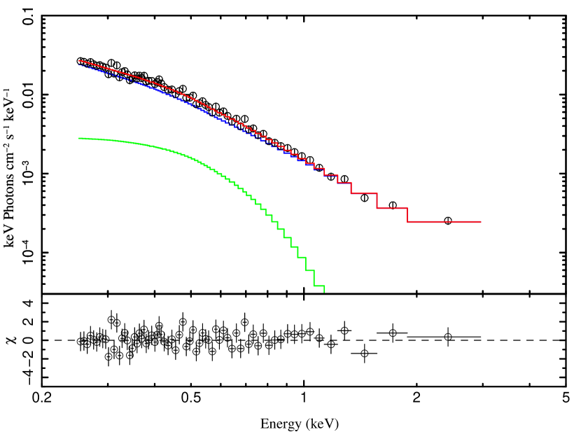
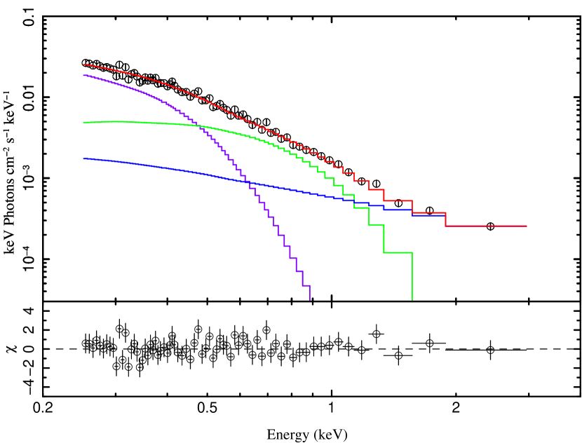
Figure 3: Left panel: Best fit blackbody+broken power-law model ($Mhi\_bb\_bkn$ in Table 1) and residuals to the high phase spectrum of RE J1034+396. The power-law component is shown by the blue histogram, the blackbody in green, and the total in red. Right panel: Best fit two blackbodies and a power-law model ($Mhi\_2bb\_pow$ in Table 1) and residuals to the same dataset shown in the left panel. The power-law component is shown by the blue histogram, the high temperature blackbody in green, the low temperature blackbody in violet, and the total in red. Please see the electronic edition of the journal for a color version of this figure.

The high phase spectrum can be well modeled with a simple blackbody of temperature $kT_{bb}=0.1^{+0.03}_{-0.02}$ keV and a broken power-law with photon index $\Gamma_{1}=3.6\pm 0.1$ below 1.9 keV and $\Gamma_{2}=1.9_{-0.9}^{+0.4}$ above 1.9 keV (also see Table 1). Hereafter this model will be referred to as $Mhi\_bb\_bkn$. While formally acceptable with $\chi^{2}/dof$ = 125.6/141, the power-law component in this model dominates not only the high energies, but also the low energies as shown in Fig. 3. Since only the peak of the blackbody contributes to the observed spectrum, replacing the blackbody with accretion disc models does not change the fits significantly. The fact that the power-law dominated both low and high energies when using a single blackbody was also noted in a previous work by Pounds et al. (1995). Following Pounds et al. (1995) we tried fitting two blackbodies with different temperature and normalizations to fit the soft ($\sim$0.3–0.9 keV) and very soft ($<$0.3 keV) energies and a power-law for the high ($>$0.9 keV) energies. The best fit parameters for this model (hereafter $Mhi\_2bb\_pow$) are presented in Table 1, and the model components and residuals are shown in Fig. 3. Note that the power-law model parameters $\Gamma_{2}$ for the model $Mhi\_bb\_bkn$, and $\Gamma$ for the model $Mhi\_2bb\_pow$ are largely constrained only by a few of the hardest energy bins, and consequently have large error bars. The 0.25–5 keV flux in the high phase spectrum is $(1.26\pm 0.1)\times 10^{-11}$ ergs/cm²/s.

3.2 Fits to the low phase spectrum

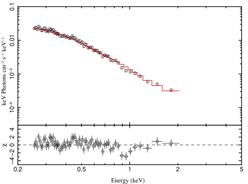
Figure 4: Left panel: Best fit to the low phase data using the model $Mhi\_bb\_bkn$ multiplied by an overall normalization constant and allowing only the normalization constant to vary, thus keeping the spectral shape same as $Mhi\_bb\_bkn$. Right panel: Same as left panel but for model $Mhi\_2bb\_pow$. In both cases note the systematic deviations in the residuals in the $\sim$0.85–1.1 keV range.

First we test if the shape of the low phase spectrum is the same as that of the high phase. For this we multiply the best-fit high phase model by an overall normalization constant and search for minimum $\chi^{2}$ allowing only this constant to change. The best-fit normalization constant has a value in the range of $0.90\pm 0.02$ for both models $Mhi\_bb\_bkn$ and $Mhi\_2bb\_pow$, when applied to the low phase spectrum. However the residuals in this case (see Fig. 4) show a systematic deviation in the $\sim$0.85–1.1 keV range, strongly suggestive of an absorption edge. There may also be some systematic deviation at lower energies, especially an edge-like absorption feature between 0.3–0.4 keV. While not statistically significant in the current dataset, if this indeed is the case then the continuum level at these energies is higher than our estimate. Some of these spectral features were also noted by Middleton et al. (2009) in the time-averaged spectrum, but coadding spectra from both high and low phases most likely lowered the observability of the features (which are prominent only during the low phase).

Noting that the 0.8–0.9 keV feature could be due to an H-like oxygen VIII K edge (at rest frame energy of 0.87 keV, seen in many Seyfert 1 sources (see e.g. Reynolds, 1997) due to presence of ionized gas in the line of sight), we next attempt to test if this feature (present only during the low phase) could indeed be due to the oxygen absorption edge. For this we included a multiplicative edge component to our models. The best-fit values after including an edge in both $Mhi\_bb\_bkn$ and $Mhi\_2bb\_pow$ are given in Table 1.

The improvement in $\chi^{2}$ fit statistic for model $Mlo\_bb\_bkn\_edge$ between $\tau=0$ (no edge) and $\tau=0.29$ (best fit) is $\Delta\chi^{2}=19.4$, implying a single parameter confidence limit of $4.4\sigma$. The improvement in $\chi^{2}$ fit statistic for $Mlo\_2bb\_pow\_edge$ between $\tau=0$ (no edge) and $\tau=0.23$ (best fit) is $\Delta\chi^{2}=16.6$, implying a single parameter confidence limit of $4.07\sigma$.

Thus both low phase models need an edge at $>$4$\sigma$ level, strongly suggesting that the edge is present in the data. While fits to both models $Mlo\_bb\_bkn$ and $Mlo\_2bb\_pow$ are formally acceptable, there remain hints of some systematic trend in the residuals shown in Fig. 4 at lower energies. This is discussed in greater detail in §4. The 0.25–5 keV flux in the low phase spectrum is $(1.14\pm 0.1)\times 10^{-11}$ ergs/cm²/s.

Next we attempted to estimate the strength of the same OVIII absorption edge in the high phase data, by adding an edge to both the models $Mhi\_bb\_bkn$ and $Mhi\_2bb\_pow$ and redoing the fits. We found that inclusion of the edge did not improve the statistical quality of the fits. The OVIII edge could not be detected (at $>3\sigma$ level) in the data using either of the continuum models, and this confirms that the optical depth of the edge varied significantly between the high and low phases.

Next we modeled the edge in the low phase somewhat more physically using the XSTAR photoionization code (Kallman & Bautista, 2001). A grid of XSTAR models was created from the following variables: (1) the column density ($N_{H}$, allowed range $10^{20}$ – $10^{23}$ cm^-2), (2) ionization parameter ($log(\xi)=log(L/(nR^{2}))$, allowed range 2–4), (3) oxygen abundance (relative to solar, allowed range 0.1–4), (4) neon abundance (relative to solar, allowed range 0.1–1). A multiplicative table model was created from this multidimensional grid. Turbulent velocities of 300 km/s and above cause absorption lines to become more prominent, and lower turbulent velocities are required to fit the data well. The best-fit parameters to the low phase data using this model in conjunction with a continuum model composed of double-blackbody+power law suggest $N_{H}$/(10²¹ cm^-2) = $4\pm 1$, log($\xi$)=$3.2_{-0.1}^{+0.2}$, and a relatively high oxygen abundance ($2.1_{-0.5}^{+0.8}$). A sub-solar neon abundance (0.13) is preferred by the best-fit solution but its error-bar could not be constrained. See Table 1 for the detailed fit parameters and statistics. The best-fit continuum parameters in this case were very similar to those obtained using the single edge model ($Mlo\_2bb\_pow$).

It is possible that oscillations in the flux of the source cause the ionization of intervening gas to vary, and that the gas is too ionized to give significant OVIII absorption during high phases. This possibility can be tested using our XSTAR model for the warm absorber gas. If this were the case, then it ought to be possible to model the high phase spectrum using the same warm absorber abundances as obtained for the best-fit to the low phase data, but with a higher ionization fraction ($\sim$10–20% higher, which is typically the flux difference between the crests and peaks). However the high phase spectrum cannot be modeled with 10–20% enhanced ionization fraction. In fact, detailed modeling shows that reasonable fits to the high phase spectrum can be obtained only if the ionization fraction is a factor of three higher than that required by the low phase spectrum. Thus it seems unlikely that the changes in the high and low phase spectrum are driven solely by flux viariations in the source.

We have also repeated the entire analyses using a different, somewhat larger exclusion radius of 35 arcseconds (smaller exclusion radii were not considered as they would be affected by pile up). In this case the errors are larger due to poorer photon statistics, but the conclusions are same, i.e. an edge is detected (at $>3\sigma$) level in the low phase, but no edge is detected in the high phase. Similarly we repeated the analyses extracting only pattern=0 events (single pixel events), and excising the PSF core of radius 30 arcseconds. In this case also the OVIII edge was detected at 4.1$\sigma$ confidence level in the low phase spectrum whereas no evidence of the OVIII edge could be found the high phase spectrum. Thus our main observation, viz. that the OVIII absorption edge is only seen during the troughs in the oscillations, and not during the crests, appears to be quite robust and is not some form of detector artifact.

4 Discussion and Conclusions

In this work we have presented phase-resolved spectroscopy of the narrow line Seyfert 1 galaxy RE J1034+396. We have used the XMM-Newton observation of this source between 2007 May 31 and 2007 June 1, when the X-ray light curve showed strong quasi-periodic oscillations. We have extracted spectra during the high (crest) and low (trough) phases. Simple continuum models assuming either a blackbody plus broken power-law, or two blackbodies plus a power-law model, fit the high phase spectrum quite well. The required low-energy power-law index is very steep ($\Gamma\sim 3.6\pm 0.1$) for a single blackbody plus broken power-law model, which is typical for narrow line AGNs with a high soft X-ray excess (Boller et al., 1996; Pounds et al., 1995; Middleton et al., 2007). The spectrum can also be well modeled using two blackbodies and a power-law continuum. Due to the steep decline of the spectrum, and high pileup on the PN detector which severely limits the photon statistics, we do not have good quality spectral data beyond $\sim$2–3 keV. Therefore for these spectra we cannot very well constrain the relatively flatter 2–10 keV continuum usually seen in this source (Crummy et al., 2006; Middleton et al., 2009), although fits to a two-blackbody plus power-law model show that the $>2$ keV spectrum is comparatively flatter with a photon index of $\sim 2$.

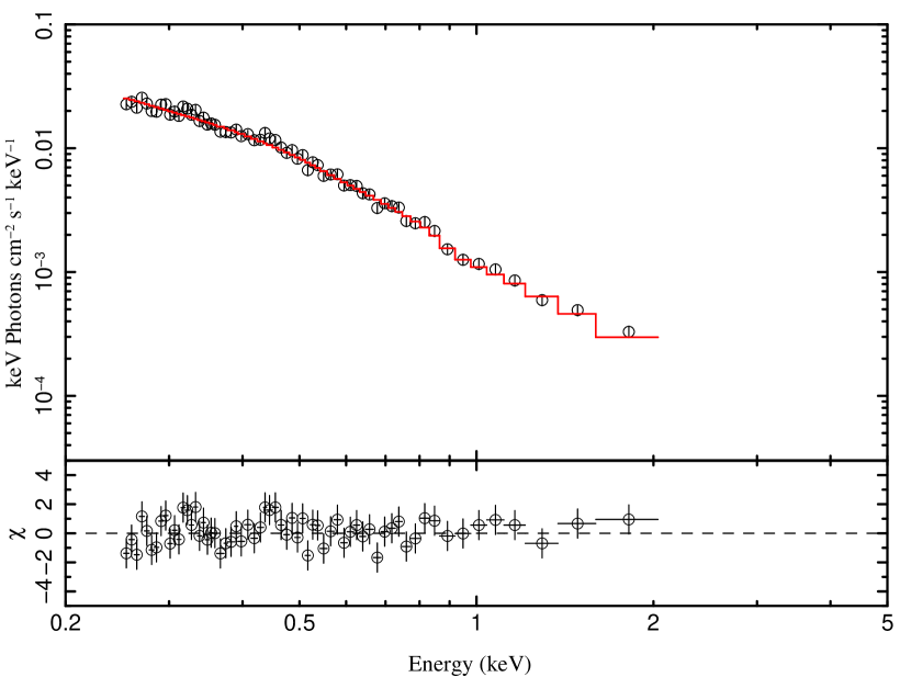
Figure 5: Best fit to the low phase data using models $Mlo\_bb\_bkn\_edge$ (left panel) and $Mlo\_2bb\_pow\_edge$ (right panel) which includes the (H-like) oxygen VIII K edge. The best fit parameters are given in Table 1.

The low phase spectrum cannot be adequately described by scaling the overall normalization of either of the best fit high phase models, suggeting that the shape of the low phase spectrum is different from that of the high phase. Analyzing the r.m.s. variability at different energies Middleton et al. (2009) also concluded that the variability is mainly from the hard photons. The right panel of Fig. 4 shows that the differences between the low and high phases are most prominent at higher energies. In particular, the residuals in Fig. 4 show a sharp drop in the continuum flux between 0.8–0.9 keV, which then slowly increases toward the expected continuum flux at higher energies, reminiscent of an absorption edge. The inclusion of an edge improves the fits significantly (at $>$4$\sigma$ level) for both single-blackbody+broken power-law model and double-blackbody+power-law model. The best fit values for the edge threshold energy and absorption depth are $0.87\pm 0.04$ keV and $0.29\pm 0.11$ respectively for the single-blackbody+broken power-law model, and $0.86^{+0.05}_{-0.06}$ keV and $0.23^{+0.12}_{-0.11}$ respectively for the double-blackbody+power-law model. The edge is most likely associated to the 0.87 keV (rest frame) K-edge of (H-like) oxygen VIII which is quite commonly seen in Seyferts (see e.g., Reynolds, 1997), and is indicative of the presence of optically thin, photoionized matter along the line of sight. RE J1034+396 however is at a redshift of 0.042; therefore the 0.87 keV edge (in rest frame) should appear at 0.84 keV (easily within the 90% confidence error bar for both models). The presence of a warm absorber should create other features in the spectrum, e.g. the 0.74 keV K edge from He-like O VII. While the residuals in Fig. 5 do show a drop in the flux, it is not very significant statistically.

To estimate the column density ($N_{\rm OVIII}$) of the O VIII ions responsible for the edge we used Eq.(1) of Verner et al. (1996) and calculated the absorption cross section $\sigma$ (for O VIII, $\sigma[{\rm E}=0.87\;{\rm keV}]=0.098$ Mb). Since $\tau=N_{\rm OVIII}\cdot\sigma$, we obtain $N_{\rm OVIII}=3\times 10^{18}$ cm^-2. Estimating the number density ($n_{\rm OVIII}$) requires a size-scale for the warm absorber. Assuming that the QPO originates in the accretion disk, the warm absorber is could be confined within the orbit of the QPO, or in case of an outflow it originates inside the QPO orbit. The mass of the supermassive black hole in RE J1034+396 is in the range of $1-7\times 10^{6}$ M_⊙ (Bian & Huang, 2010; Zhou et al., 2010). A circular Keplerian orbit would have a radius of $9.4(M/[4\times 10^{6}M_{\odot}])^{-2/3}(P/[1hr])^{2/3}\;r_{\rm g}$, which would be an upper limit on the size of the absorber in this case. This would give $n_{\rm OVIII}=3\times 10^{5}$ cm^-3 for the number density of OVIII ions. Note however that this assumes a Keplerian orbit origin for the QPO, and therefore depends on the mass of the central supermassive black hole. Thus in RE J1034+396 we may be seeing an infalling “blob”, the emission from which is periodically absorbed as it passes behind a warm absorber in the immediate vicinity of the central engine. If the “blob” is at $\sim$9 $r_{\rm g}$, that would imply the ionizing flux must be generated within 9 $r_{\rm g}$ (or else we would not see absorption), and this would be easier to accomplish if the black hole is spinning since the disk can get down to a smaller radius (e.g. as low as 1.25 $r_{\rm g}$ for a maximally spinning black hole). Recent work by Crummy et al. (2006) has shown that NLS1 spectra can be modeled using reflection from a disk around a spinning black holes (see Miller, 2007, for a review).

We also created a multidimensional grid of models using the XSTAR photoionization code, to create a more physical model for the warm absorber and explore a wide range of column density, ionization parameter, oxygen and neon abundance. Fits to the low-phase data using this model suggests a warm absorber column density of $\sim 4\times 10^{21}$ cm^-2, log($\xi$)=$3.2_{-0.1}^{+0.2}$, and an oxygen abundance of $2.1_{-0.5}^{+0.8}$ relative to solar. The neon abundance could not be well constrained from the data, although the best-fit solution suggests a sub-solar value.

Another possible physical scenario for the difference between high and low phase spectrum could be that the warm absorber is along the line of sight, between us and the source (where the QPO originates), and the warm absorber responds to flux variations in the source itself, i.e. it is more ionized and transparent at high fluxes and less at lower fluxes. However, based on our modeling of the spectra using physically motivated models generated using XSTAR this scenario appears unlikely because the change in luminosity of the ionizing flux between low and high phases is too small to create the observed difference in the depth of the OVIII edge (also see §3).

It is interesting to note in this context that a somewhat complementary situation has been observed in the Seyfert galaxy NGC 1365, where Risaliti et al. (2009) have reported a possible transit of an obscuring cloud (with $N_{H}\sim 3.5\times 10^{23}$ cm^-2 and other inferred properties similar to that of a broad-line region cloud) in front of the central X-ray source.

Signatures of variable absorption on short timescales have been previously observed in high resolution Chandra spectra of the stellar black hole candidate H1743–22 (Miller et al., 2006). For H1743–22, the lines were slightly blueshifted, suggesting an outflow origin. For RE J1034+396, we do not have definitive evidence for an outflow, but the best fit edge energy for both models is higher (though within 90% confidence interval) than the rest frame energy of the oxygen edge. If the warm absorber in RE J1034+396 is indeed in an outflow, then the observed oscillations could originate due to an instability in the inner accretion disk threaded by a poloidal magnetic field, giving rise to an outflowing wind or jet (Blandford & Payne, 1982; Tagger & Pellat, 1999). The observed oscillations in this case would correspond to scaled up versions of low-frequency QPOs (see e.g., van der Klis, 2006) seen in stellar mass X-ray binaries.

Since the presence of a warm absorber is bound to have noticeable imprints on other regions of the electromagnetic spectrum, especially in UV and soft X-rays, future deep UV and X-ray observations of RE J1034+396 will be useful not only in constraining the origin of the oscillations, but also in gaining a better understanding of the physical emission mechanism of sources like RE J1034+396 which show a strong soft-X-ray excess. Future X-ray missions with improved sensitivity and larger collecting area like the International X-ray Observatory (IXO; Miller et al., 2009; White et al., 2010) would play key role in understanding accretion geometry as well as emission/absorption mechanism in these sources.

Table 1: Summary of fits.

Phase	Model	Best-fit parameters	Best-fit statistics
High	$Mhi\_bb\_bkn$	$kT_{bb}=0.1_{-0.02}^{+0.03}$
		$N_{bb}/10^{-5}=3.2_{-1.7}^{+2.9}$
		$\Gamma_{1}=3.6\pm 0.1$
		$N_{p}/10^{-3}=1.5\pm 0.1$
		$E_{b}=1.9_{-0.3}^{+0.6}$
		$\Gamma_{2}=1.9_{-0.9}^{+0.4}$
			$\chi^{2}/\nu=125.6/141$
High	$Mhi\_2bb\_pow$	$kT_{bb1}=0.06\pm 0.01$
		$N_{bb1}/10^{-4}=2.8^{+0.4}_{-0.3}$
		$kT_{bb2}=0.14\pm 0.02$
		$N_{bb2}/10^{-5}=6.9^{+1.6}_{-1.3}$
		$\Gamma=2.0\pm 0.4$
		$N_{p}/10^{-4}=6^{+3}_{-2}$
			$\chi^{2}/\nu=130.0/141$
Low	$Mlo\_bb\_bkn\_edge$	$kT_{bb}=0.09_{-0.01}^{+0.01}$
		$N_{bb}/10^{-5}=2.9_{-0.4}^{+0.5}$
		$N_{p}/10^{-3}=1.3\pm 0.2$
		$\Gamma_{1}=3.6\pm 0.03$
		$E_{b}=1.8_{-0.2}^{+0.7}$
		$\Gamma_{2}=2.3\pm 0.5$
		$E_{e}$ = $0.87\pm 0.04$
		$\tau=0.29\pm 0.11$
			$\chi^{2}/\nu=136.0/128$
Low	$Mlo\_2bb\_pow\_edge$	$kT_{bb1}=0.06_{-0.02}^{+0.01}$
		$N_{bb1}/10^{-4}=2.4_{-0.0}^{+0.1}$
		$kT_{bb2}=0.14\pm 0.04$
		$N_{bb2}/10^{-5}=5.6\pm 0.2$
		$\Gamma=2.36_{-0.58}^{+0.06}$
		$N_{p}/10^{-4}=6.7_{-2.7}^{+0.4}$
		$E_{e}$ = $0.86_{-0.06}^{+0.05}$
		$\tau=0.23_{-0.11}^{+0.12}$
			$\chi^{2}/\nu=133.6/128$
Low	$Mlo\_2bb\_pow\_xsgrid$	$kT_{bb1}=0.06\pm 0.01$
		$N_{bb1}/10^{-4}=2.4_{-0.0}^{+0.1}$
		$kT_{bb2}=0.14\pm 0.01$
		$N_{bb2}/10^{-5}=5.6_{0}^{+0.2}$
		$\Gamma=2.42_{-0.51}^{+0.01}$
		$N_{p}/10^{-4}=7.4\pm 0.4$
		$N_{H}/10^{21}=4\pm 1$
		log($\xi$) = $3.2_{-0.1}^{+0.2}$
		O${}_{\rm Abund}=2.1_{-0.5}^{+0.8}$
		Ne${}_{\rm Abund}=0.14_{-0.04}^{+0.86}$
			$\chi^{2}/\nu=134.3/126$

Figure 1: The red line shows the 9 point moving averaged light curve extracted from EPIC PN data, from a circular region of 45 arcsecond radius around the source, i.e. before excising the central, piled up core of the PSF. The start time here corresponds to 2007 May 31, 20:11:01 UTC. The high and low phases selected using the algorithm described in §2 are shown in light red and light blue respectively. Please see the electronic edition of the journal for a color version of this figure.

Figure 2: An example showing the selection of good time interval near a trough, following the algorithm described in §2.

References

- Bian & Huang (2010) Bian, W.-H., & Huang, K. 2010, MNRAS, 401, 507
- Blandford & Payne (1982) Blandford, R. D., & Payne, D. G. 1982, MNRAS, 199, 883
- Boller et al. (1996) Boller, T., Brandt, W. N., & Fink, H. 1996, A&A, 305, 53
- Crummy et al. (2006) Crummy, J., Fabian, A. C., Gallo, L., & Ross, R. R. 2006, MNRAS, 365, 1067
- Gierliński et al. (2008) Gierliński, M., Middleton, M., Ward, M., & Done, C. 2008, Nature, 455, 369
- Houck & Denicola (2000) Houck, J. C., & Denicola, L. A. 2000, Astronomical Data Analysis Software and Systems IX, 216, 591
- Kallman & Bautista (2001) Kallman, T., & Bautista, M. 2001, ApJS, 133, 221
- Middleton et al. (2007) Middleton, M., Done, C., & Gierliński, M. 2007, MNRAS, 381, 1426
- Middleton et al. (2009) Middleton, M., Done, C., Ward, M., Gierliński, M., & Schurch, N. 2009, MNRAS, 394, 250
- Middleton & Done (2009) Middleton, M., & Done, C. 2009, arXiv:0908.0224
- Miller (2007) Miller, J. M. 2007, ARA&A, 45, 441
- Miller & Homan (2005) Miller, J. M., & Homan, J. 2005, ApJ, 618, L107
- Miller et al. (2006) Miller, J. M., et al. 2006, ApJ, 646, 394
- Miller et al. (2009) Miller, J., et al. 2009, astro2010: The Astronomy and Astrophysics Decadal Survey, 2010, 208
- Morgan et al. (1997) Morgan, E. H., Remillard, R. A., & Greiner, J. 1997, ApJ, 482, 993
- Osterbrock & Pogge (1985) Osterbrock, D. E., & Pogge, R. W. 1985, ApJ, 297, 166
- Pounds et al. (1995) Pounds, K. A., Done, C., & Osborne, J. P. 1995, MNRAS, 277, L5
- Puchnarewicz et al. (1998) Puchnarewicz, E. M., Mason, K. O., & Siemiginowska, A. 1998, MNRAS, 293, L52
- Puchnarewicz et al. (1995) Puchnarewicz, E. M., Mason, K. O., Siemiginowska, A., & Pounds, K. A. 1995, MNRAS, 276, 20
- Proga & Kallman (2004) Proga, D., & Kallman, T. R. 2004, ApJ, 616, 688
- Reeves et al. (2008) Reeves, J., Done, C., Pounds, K., Terashima, Y., Hayashida, K., Anabuki, N., Uchino, M., & Turner, M. 2008, MNRAS, 385, L108
- Reynolds (1997) Reynolds, C. S. 1997, MNRAS, 286, 513
- Risaliti et al. (2009) Risaliti, G., et al. 2009, ApJ, 696, 160
- Ross & Fabian (1993) Ross, R. R., & Fabian, A. C. 1993, MNRAS, 261, 74
- Schurch & Done (2007) Schurch, N. J., & Done, C. 2007, MNRAS, 381, 1413
- Shakura & Sunyaev (1973) Shakura, N. I., & Sunyaev, R. A. 1973, A&A, 24, 337
- Tagger & Pellat (1999) Tagger, M., & Pellat, R. 1999, A&A, 349, 1003
- Titarchuk (1994) Titarchuk, L. 1994, ApJ, 434, 570
- van der Klis (2006) van der Klis, M. 2006, In: Compact Stellar X-ray Sources, Cambridge Astrophysics Series, 39, Cambridge University Press
- Verner et al. (1996) Verner, D. A., Ferland, G. J., Korista, K. T., & Yakovlev, D. G. 1996, ApJ, 465, 487
- Watarai et al. (2000) Watarai, K.-y., Fukue, J., Takeuchi, M., & Mineshige, S. 2000, PASJ, 52, 133
- White et al. (2010) White, N. E., Parmar, A., Kunieda, H., Nandra, K., Ohashi, T., & Bookbinder, J. 2010, arXiv:1001.2843
- Zhou et al. (2010) Zhou, X.-L., Zhang, S.-N., Wang, D.-X., & Zhu, L. 2010, ApJ, 710, 16