Physical properties of ESA Rosetta target asteroid (21) Lutetia: Shape and flyby geometry

Abstract

Aims. We determine the physical properties (spin state and shape) of asteroid (21) Lutetia, target of the ESA Rosetta mission, to help in preparing for observations during the flyby on 2010 July 10 by predicting the orientation of Lutetia as seen from Rosetta.

Methods. We use our novel KOALA inversion algorithm to determine the physical properties of asteroids from a combination of optical lightcurves, disk-resolved images, and stellar occultations, although the latter are not available for (21) Lutetia.

Results. We find the spin axis of (21) Lutetia to lie within 5° of ($\lambda=52$°, $\beta=-6$°) in Ecliptic J2000 reference frame (equatorial $\alpha=52$°, $\delta=+12$°), and determine an improved sidereal period of 8.168 270 $\pm$ 0.000 001 h. This pole solution implies the southern hemisphere of Lutetia will be in “seasonal” shadow at the time of the flyby. The apparent cross-section of Lutetia is triangular as seen “pole-on” and more rectangular as seen “equator-on”. The best-fit model suggests the presence of several concavities. The largest of these is close to the north pole and may be associated with large impacts.

1 Introduction

The origin and evolution of the Solar System and its implications for early planetesimal formation are key questions in planetary science. Unlike terrestrial planets, which have experienced significant mineralogical evolution, through endogenic activity, since their accretion, small Solar System bodies have remained essentially unaltered. Thus, a considerable amount of information regarding the primordial planetary processes that occurred during and immediately after the accretion of the early planetesimals is still present among this population. Consequently, studying asteroids is of prime importance in understanding the planetary formation processes [Bottke et al. 2002] and, first and foremost, requires a reliable knowledge of their physical properties (size, shape, spin, mass, density, internal structure, etc.) in addition to their compositions and dynamics. Statistical analyses of these parameters for a wide range of asteroids can provide relevant information about inter-relationships and formation scenarios.
In this respect, our observing program with adaptive optics, allowing diffraction-limited observations from the ground with 10 m-class telescopes, has now broken the barrier which separated asteroids from real planetary worlds [e.g., Conrad et al. 2007; Carry et al. 2008; Drummond et al. 2009; Carry et al. 2010; Drummond et al. 2010]. Their shapes, topography, sizes, spins, surface features, albedos, and color variations can now be directly observed from the ground. This opens these objects to geological, rather than astronomical-only, study. While such surface detail is only possible for the largest asteroids, our main focus is on determining accurately the size, shape, and pole. Among them, we have observed (21) Lutetia, an asteroid that will be observed in-situ by the ESA Rosetta mission.
The Rosetta Mission will encounter its principal target, the comet 67P/Churyumov-Gerasimenko, in 2014. However, its interplanetary journey was designed to allow close encounters with two main-belt asteroids: (2867) Šteins and (21) Lutetia. The small asteroid (2867) Šteins was visited on 2008 September 5 at a minimum distance of about 800 km [Schulz et al. 2009] and (21) Lutetia will be encountered on 2010 July 10. Knowing the geometry of the flyby (e.g., visible hemisphere, sub-spacecraft coordinates as function of time, and distance) before the encounter is crucial to optimize the observation sequence and schedule the on-board operations. The size of Lutetia [estimated at $\sim$100 km, see Tedesco et al. 2002, 2004; Mueller et al. 2006] allows its apparent disk to be spatially resolved from Earth. Our goal is therefore to improve knowledge of its physical properties to prepare for the spacecraft flyby.
Lutetia, the Latin name for the city of Paris, is a main-belt asteroid (semi-major axis 2.44 AU) that has been studied extensively from the ground [see Barucci et al. 2007, for a review, primarily of recent observations]. Numerous studies have estimated indirectly its spin [by lightcurve, e.g., Lupishko et al. 1987; Dotto et al. 1992; Torppa et al. 2003]. Size and albedo were reasonably well determined in the 1970s by Morrison [1977] using thermal radiometry (108–109 km), and by Zellner & Gradie [1976] using polarimetry (110 km). Five somewhat scattered IRAS scans [e.g., Tedesco et al. 2002, 2004] yielded a higher albedo and smaller size than the dedicated observations in the 1970s. Mueller et al. [2006] derived results from new radiometry that are roughly compatible with the earlier results or with the IRAS results, depending on which thermal model is used. Carvano et al. [2008] later derived a lower albedo from ground-based observations, seemingly incompatible with previous works. Radar data analyzed by Magri et al. [1999, 2007] yielded an effective diameter for Lutetia of 116 km; reinterpretation of those data and new radar observations [Shepard et al. 2008] suggest an effective diameter of 100 $\pm$ 11 km and an associated visual albedo of 0.20. Recent HST observations of Lutetia [Weaver et al. 2009] indicate a visual albedo of about 16%, a result based partly on the size/shape/pole determinations from our work in the present paper and Drummond et al. [2010].
Lutetia has been extensively studied using spectroscopy in the visible, near- and mid-infrared and its albedo measured by polarimetry and thermal radiometry [McCord & Chapman 1975; Chapman et al. 1975; Zellner & Gradie 1976; Bowell et al. 1978; Rivkin et al. 1995; Magri et al. 1999; Rivkin et al. 2000; Lazzarin et al. 2004; Barucci et al. 2005; Birlan et al. 2006; Nedelcu et al. 2007; Barucci et al. 2008; Shepard et al. 2008; DeMeo et al. 2009; Vernazza et al. 2009; Lazzarin et al. 2009, 2010; Perna et al. 2010; Belskaya et al. 2010]. We present a discussion on Lutetia’s taxonomy and composition in a companion paper [Drummond et al. 2010].
Thermal infrared observations used to determine the size and albedo of Lutetia were initially inconsistent, with discrepancies in diameters and visible albedos reported [e.g., Zellner & Gradie 1976; Lupishko & Belskaya 1989; Belskaya & Lagerkvist 1996; Tedesco et al. 2002; Mueller et al. 2006; Carvano et al. 2008]. Mueller et al. [2006] and Carvano et al. [2008], however, interpreted these variations as an indication of surface heterogeneity, inferring that the terrain roughness of Lutetia increased toward northern latitudes, that the crater distribution is different over the northern/southern hemispheres, and includes a possibility of one or several large craters in Lutetia’s northern hemisphere. Indeed, the convex shape model derived from the inversion of 32 optical lightcurves [Torppa et al. 2003] displays a flat top near the north pole of Lutetia. Kaasalainen et al. [2002] have shown that large flat regions in these convex models could be a site of concavities. The southern hemisphere is not expected to be free from craters however, as Perna et al. [2010] detected a slight variation of the visible spectral slope, possibly due to the presence of large craters or albedo spots in the southern hemisphere.
In this paper, we present simultaneous analysis of adaptive-optics images obtained at the W. M. Keck and the European Southern Observatory (ESO) Very Large Telescope (VLT) observatories, together with lightcurves, and we determine the shape and spin state of Lutetia. In section 2, we present the observations, in section 3 the shape of Lutetia, and finally, we describe the geometry of the upcoming Rosetta flyby in section 4.

2 Observations and data processing

2.1 Disk-resolved imaging observations

We have obtained high angular-resolution images of the apparent disk of (21) Lutetia over six nights during its last opposition (late 2008 - early 2009) at the W. M. Keck Observatory with the adaptive-optics-fed NIRC2 camera [$9.942\pm 0.050$ milli-arcsecond per pixel, van Dam et al. 2004]. We also obtained data in 2007 [Perna et al. 2007] at the ESO VLT with the adaptive-optics-assisted NACO camera [$13.27\pm 0.050$ milli-arcsecond per pixel, Rousset et al. 2003; Lenzen et al. 2003]. We list observational circumstances for all epochs in Table 1. Although the AO data used here are the same as in Drummond et al. [2010], we analyze them with an independent approach. We do not use our 2000 epoch, however, from Keck (NIRSPEC instrument) because those data were taken for the purpose of a search for satellites and therefore the Point-Spread Function (PSF) calibrations were not adequate for shape recovery.

Table 1: Heliocentric distance ($r$), range to observer ($\Delta$), solar phase angle ($\alpha$), apparent visual magnitude (m_V), angular diameter ($\phi$), coordinates (longitude $\lambda$ and latitude $\beta$) of the Sub-Earth Point (SEP) and Sub-Solar Point (SSP), for each epoch (mean time listed in UT, without light-time correction). All the data were obtained at W. M. Keck observatory, except the 2007 epochs, which were obtained at ESO Very Large Telescope.

Date	$r$	$\Delta$	$\alpha$	mV	$\phi$	SEPλ	SEPφ	SSPλ	SSPφ
(UT)	(AU)	(AU)	(°)	(mag)	(″)	(°)	(°)	(°)	(°)
2007-06-06T00:19	2.30	1.30	3.2	10.1	0.14	339	73	337	70
2007-06-06T02:56	2.30	1.30	3.2	10.1	0.14	223	73	221	70
2007-06-06T06:45	2.30	1.30	3.3	10.1	0.14	55	73	53	70
2007-06-06T08:08	2.30	1.30	3.3	10.1	0.14	354	73	352	70
2007-06-06T08:16	2.30	1.30	3.3	10.1	0.14	348	73	346	70
2007-06-06T08:22	2.30	1.30	3.3	10.1	0.14	344	73	342	70
2007-06-06T08:27	2.30	1.30	3.3	10.1	0.14	340	73	338	70
2008-10-22T15:14	2.36	1.55	17.9	11.1	0.12	267	-65	298	-82
2008-10-22T15:20	2.36	1.55	17.9	11.1	0.12	263	-65	294	-82
2008-10-22T15:25	2.36	1.55	17.9	11.1	0.12	259	-65	290	-82
2008-10-22T15:33	2.36	1.55	17.9	11.1	0.12	253	-65	284	-82
2008-11-21T10:39	2.41	1.43	4.7	10.5	0.13	61	-70	68	-75
2008-12-02T07:05	2.43	1.44	1.1	10.2	0.13	106	-73	106	-72
2008-12-02T07:12	2.43	1.44	1.1	10.2	0.13	100	-73	101	-72
2008-12-02T07:29	2.43	1.44	1.1	10.2	0.13	89	-73	89	-72
2008-12-02T07:35	2.43	1.44	1.1	10.2	0.13	84	-73	84	-72
2008-12-02T07:49	2.43	1.44	1.1	10.2	0.13	74	-73	74	-72
2008-12-02T07:54	2.43	1.44	1.1	10.2	0.13	70	-73	70	-72
2008-12-02T08:07	2.43	1.44	1.1	10.2	0.13	61	-73	61	-72
2008-12-02T08:12	2.43	1.44	1.1	10.2	0.13	57	-73	57	-72
2008-12-02T08:18	2.43	1.44	1.1	10.2	0.13	53	-73	53	-72
2008-12-02T08:23	2.43	1.44	1.1	10.2	0.13	49	-73	49	-72
2008-12-02T08:28	2.43	1.44	1.1	10.2	0.13	45	-73	46	-72
2008-12-02T08:34	2.43	1.44	1.1	10.2	0.13	41	-73	41	-72
2008-12-02T08:39	2.43	1.44	1.1	10.2	0.13	37	-73	37	-72
2008-12-02T08:45	2.43	1.44	1.1	10.2	0.13	33	-73	33	-72
2008-12-02T08:50	2.43	1.44	1.1	10.2	0.13	29	-73	29	-72
2008-12-02T08:56	2.43	1.44	1.1	10.2	0.13	25	-73	25	-72
2008-12-02T09:01	2.43	1.44	1.1	10.2	0.13	21	-73	21	-72
2008-12-02T09:07	2.43	1.44	1.1	10.2	0.13	17	-73	17	-72
2008-12-02T09:12	2.43	1.44	1.1	10.2	0.13	13	-73	13	-72
2009-01-23T06:24	2.52	1.89	20.1	11.8	0.10	232	-78	209	-59
2009-01-23T09:17	2.52	1.90	20.1	11.8	0.10	105	-78	82	-59
2009-02-02T08:35	2.54	2.03	21.6	12.0	0.09	357	-77	336	-57
2009-02-02T08:41	2.54	2.03	21.6	12.0	0.09	352	-77	331	-57
2009-02-02T08:45	2.54	2.03	21.6	12.0	0.09	350	-77	328	-57

We reduced the data using usual procedures for near-infrared images, including bad pixel removal, sky subtraction, and flat-fielding [see Carry et al. 2008, for a more detailed description]. We then restored the images to optimal angular-resolution using the Mistral deconvolution algorithm [Conan et al. 2000; Mugnier et al. 2004]. The validity of this approach (real-time Adaptive-Optics correction followed by a posteriori deconvolution) has already been demonstrated elsewhere [Marchis et al. 2002; Witasse et al. 2006]. Although PSF observations were not available close in time to each Lutetia observation and could lead to a possible bias on the apparent size of Lutetia, two lines of evidence provide confidence in our results. First, we note that the Next-Generation Wave-Front Controller [NGWFC, van Dam et al. 2007] of NIRC2 provides stable correction and therefore limits such biases. Second, the image analysis presented in Drummond et al. [2010],which does not rely on separately measured PSF profiles [Parametric Blind Deconvolution, see Drummond 2000], confirms our overall size and orientation of Lutetia on the plane of the sky at each epoch. We are thus confident in the large scale features presented by the shape model derived below.
In total, we obtained 324 images of (21) Lutetia on 7 nights over 2007-2009 (Table 1). A subset of the restored images is presented in Fig. 1.

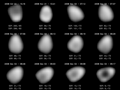
Figure 1: Selected views of (21) Lutetia in the near-infrared. All the images have been deconvolved with Mistral to enhance the definition of the edges. No effort has been made to restore photometric accuracy over the apparent disk and some ringing effects can be seen in the frames. However, this does not influence the shape of the derived contours. All images have been scaled to display the same apparent size and rotated so that the projection of the rotation axis is directed toward the top of the page (the observer is still viewing from above high southern latitudes, i.e., largely pole-on, and so, in 3D, the spin axis is mostly directed out of the page). Observing time (UT), Sub-Earth Point (SEP), and Sub-Solar Point (SSP) coordinates are listed on each frame.

2.2 Optical lightcurve observations

We utilized all 32 optical lightcurves from Torppa et al. [2003] to derive the convex shape of (21) Lutetia from lightcurve inversion [Kaasalainen & Torppa 2001; Kaasalainen et al. 2001]. We present these lightcurves in Fig. 4, together with 18 additional lightcurves acquired subsequent to ESA’s decision to target Lutetia. Some of the new data were taken in 2007 January by the OSIRIS camera on-board Rosetta during its interplanetary journey [Faury et al. 2009]. Eight lightcurves come from the CDR-CDL group led by Raoul Behrend at the Geneva observatory. The aim of this group is to organize photometric observations (including those from many amateurs) for selected asteroids and to search for binary objects [Behrend et al. 2006]. The result is two full composite lightcurves in 2003 and 2010 covering Lutetia’s period. Six other lightcurves come from the Pic du Midi 1m telescope in 2006 [Nedelcu et al. 2007] and 2009 (new data presented here). See Fig. 4 for a detailed listing of the observations. In total we used 50 lightcurves spread over years 1962-2010.

2.3 The KOALA method

We use a novel method to derive physical properties of asteroids from a combination of disk-resolved images, stellar occultation chords and optical lightcurves, called KOALA (for Knitted Occultation, Adaptive-optics, and Lightcurve Analysis). A complete description of the method can be found elsewhere [Kaasalainen 2010], as well as an example of its application on (2) Pallas [Carry et al. 2010].
We first extracted the contour of (21) Lutetia on each image using a Laplacian of Gaussian wavelet [see Carry et al. 2008, for more detail about this method]. These contours provide a direct measurement of Lutetia’s size and shape at each epoch (Table 1). Stellar occultations also provide similar constraints if several chords per event are observed. Unfortunately, there are only two archived stellar occultations by Lutetia [Dunham & Herald 2009] with only one chord each that do not provide useful constraints. The optical lightcurves bring indirect constraints on the shape of Lutetia, provided the albedo is homogeneous over its surface. Indeed, lightcurves are influenced by a combination of the asteroid shape and albedo variation [see the discussion by Carry et al. 2010, regarding the effect of albedo features on the shape reconstruction].
Slight spectral heterogeneity has been reported from visible and near-infrared spectroscopy [Nedelcu et al. 2007; Perna et al. 2010; Lazzarin et al. 2010], spanning several oppositions and hence Sub-Earth Point (SEP) latitudes and longitudes. Although Belskaya et al. [2010] claim that Lutetia’s surface is highly heterogeneous, they indicate that there is no strong evidence for large variations in albedo over the surface. They argue that the observed level of albedo variation is consistent with variations in regolith texture or minerology. We therefore assume homogeneously distributed albedo features on the surface (valid for variations of small amplitude) and that lightcurves are influenced by the shape of Lutetia only.

3 Shape and spin of (21) Lutetia

The shape of asteroid (21) Lutetia is well described by a wedge of Camembert cheese (justifying the Parisian name of Lutetia), as visible in Fig. 2. The shape model derived here suggests the presence of several large concavities on the surface of Lutetia, presumably resulting from large cratering events.
The major feature (#1, see Fig. 2) is a large depression situated close to the north pole around (10°,+60°), suggesting the presence of one or several craters, and giving a flat-topped shape to Lutetia. Mueller et al. [2006] and Carvano et al. [2008] found the surface of the northern hemisphere to be rougher than in the southern hemisphere, possibly due to the presence of large crater(s). Two other large features are possible: the second largest feature (#2) lies at (300°, -25°), and the third (#3) at (20°, -20°).
This shape model provides a very good fit to disk-resolved images (Fig. 3) and optical lightcurves (Fig. 4). The root mean square (RMS) deviations for the two modes of data are, 3.3 km (0.3 pixel) for imaging and 0.15 magnitude (1.7 % relative deviation) for lightcurves. The overall shape compellingly matches the convex shape derived by Torppa et al. [2003], and the pole solution derived here lies 18 degrees from the synthetic solution from Kryszczyńska et al. [2007], based mainly on indirect determinations.
An ellipsoid approximation to the 3D shape model has dimensions $124\times 101\times 80$ km (we estimate the 1 sigma uncertainties to be about $\pm$ $5\times 5\times 15$ km). We note here that dimension along the shortest ($c$) axis of Lutetia is much more poorly constrained here than the $a$ and $b$ axes. Indeed, all the disk-resolved images were obtained with high Sub-Earth Point latitudes ($|$SEP${}_{\beta}|\geq 65$°, “pole-on” views) and we, therefore, have limited knowledge of the size of Lutetia along its rotation axis. Hence, shape models of Lutetia with $b/c$ axes ratio ranging from 1.1 to 1.3 are not invalidated by our observations (all the values and figures presented here are for the model with $b/c=1.2$). Higher values of $b/c$ decrease the quality of the fit, and although lower values are possible (Belskaya et al. [2010] even suggested $b/c$ should be smaller than 1.1), the algorithm begins to break down: (a) spurious localized features appear (generated by the lack of shape constraints along meridians), and (b) the spin axis begins to show large departures from the short axis and would be dynamically unstable. A complete discussion on the size and density of (21) Lutetia is presented in Drummond et al. [2010]. To better constrain the $c$-dimension, we combine the best attributes of our KOALA model and our triaxial ellipsoid model to create a hybrid shape model, with ellipsoid-approximated dimensions 124 $\times$ 101 $\times$ 93 km, and thus having an average diameter of 105 $\pm$ 5 km.
We list in Table 2 the spin solution we find. The high precision (3 ms) on sidereal period results from the long time-line (47 years) of lightcurve observations. This solution yields an obliquity of 95°, Lutetia being being tilted with respect to its orbital plane, similar to Uranus. Consequently, the northern/southern hemispheres of Lutetia experience long seasons, alternating between constant illumination (summer) and constant darkness (winter) while the asteroid orbits around the Sun. This has strong implications for the Rosetta flyby, as described in the following section.

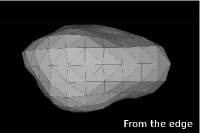
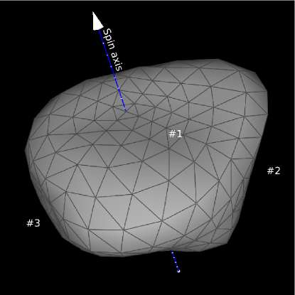
Figure 2: A view of Lutetia’s shape model obtained with the KOALA algorithm The three possible concavities listed in the text are labeled here. The view from the ”top” means a view from above the north pole.

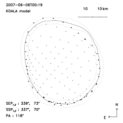
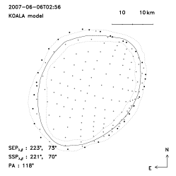
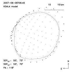
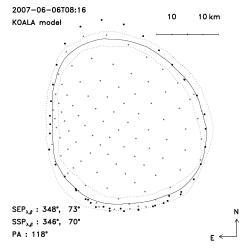
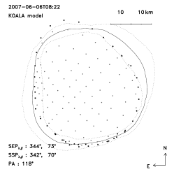
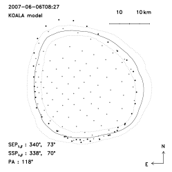
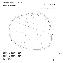
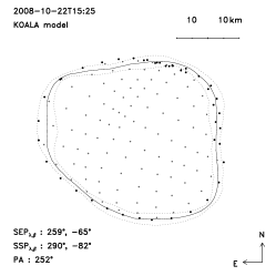
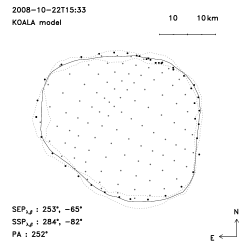
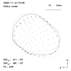
(a) First set of Lutetia contours

Figure 3: Comparison of the KOALA shape model of (21) Lutetia to the contours extracted on the adaptive-optics images. Each vertex of the shape model is represented by a grey dot, with the exception of limb/terminator vertices, which are drawn as black dots. The median AO-contour for each epoch is plotted as a solid grey line, and the 3 $\sigma$ deviation area is delimited by the dotted grey lines. We report the observing time (in UT), Sub-Earth Point (SEP), Sub-Solar Point (SSP) coordinates and Pole Angle (PA: defined as the angle in the plane of the sky between celestial north and the projected asteroid spin-vector, measured counter-clockwise, from north through east) on each frame.

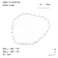
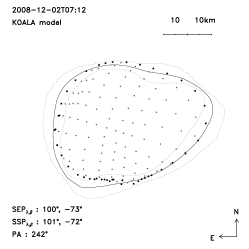
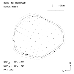
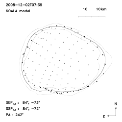
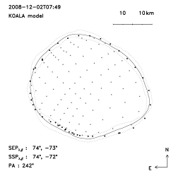
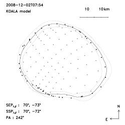
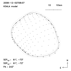
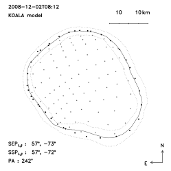
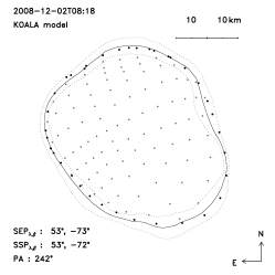
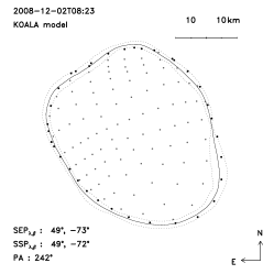
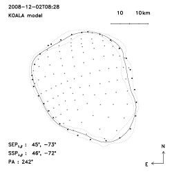
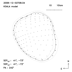
(b) Second set of Lutetia contours

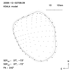
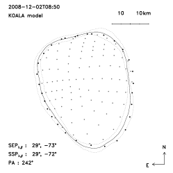
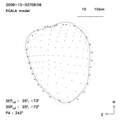
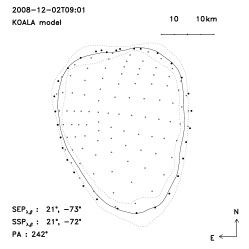
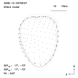
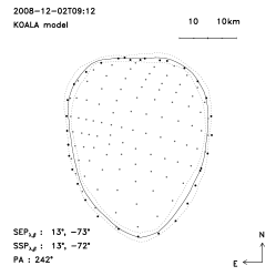
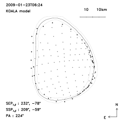
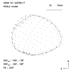
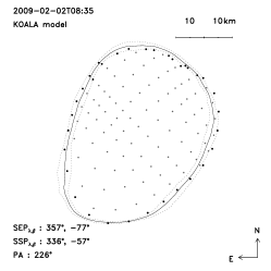
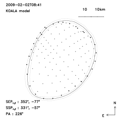
(c) Third set of Lutetia contours

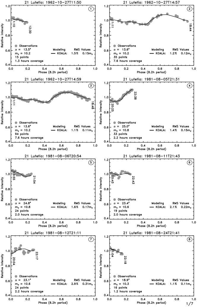
(a) First set of lightcurves (1962–1981)

Figure 4: Synthetic lightcurves obtained with the KOALA model plotted against the 50 lightcurves used in the current study, plotted in arbitrary relative intensity. The observing conditions (phase angle $\alpha$, average apparent visual magnitude $m_{V}$, number of points and duration of the observation) of each lightcurve are reported on each panel, along with the synthetic lightcurve fit RMS (in percent and visual magnitude). Lightcurve observations were acquired by $(1-3)$ Chang & Chang [1963] $(4-9)$ Lupishko et al. [1983], $(10-11)$ Zappala et al. [1984], $(12)$ Lupishko et al. [1983], $(13)$ Zappala et al. [1984], $(14-15)$ Lupishko et al. [1987], $(16)$ Dotto et al. [1992], $(17-21)$ Lupishko & Velichko [1987], $(22)$ Lagerkvist et al. [1995], $(23)$ Lupishko & Velichko [1987], $(24)$ Lagerkvist et al. [1995], $(25-28)$ Denchev et al. [1998], $(29-32)$ Denchev [2000] $(33-36)$ L. Bernasconi, $(37)$ R. Roy, $(38)$ Carvano et al. [2008], $(39-40)$ Nedelcu et al. [2007], $(41)$ OSIRIS on Rosetta [Faury et al. 2009], $(42)$ Belskaya et al. [2010], $(43-46)$ F. Colas, F. Vachier, A. Kryszczynska and M. Polinska, $(47)$ R. Poncy, $(48-49)$ R. Naves, $(50)$ P. Wiggins

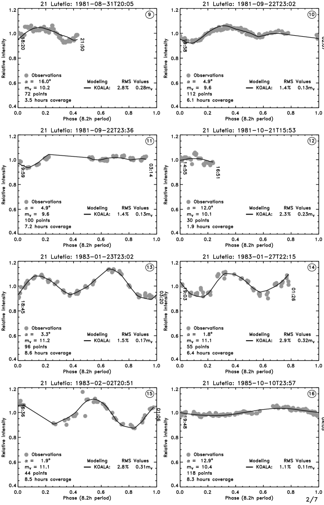
(b) Second set of lightcurves (1981–1985)

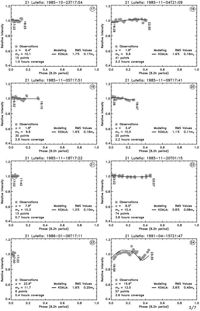
(c) Third set of lightcurves (1985–1991)

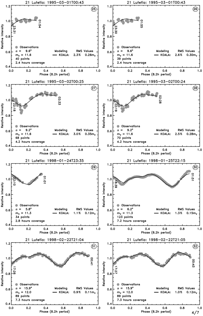
(d) Fourth set of lightcurves (1995–1998)

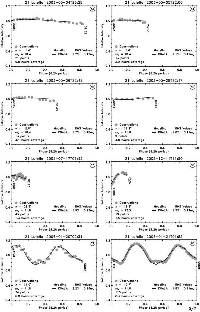
(e) Fifth set of lightcurves (2003–2006)

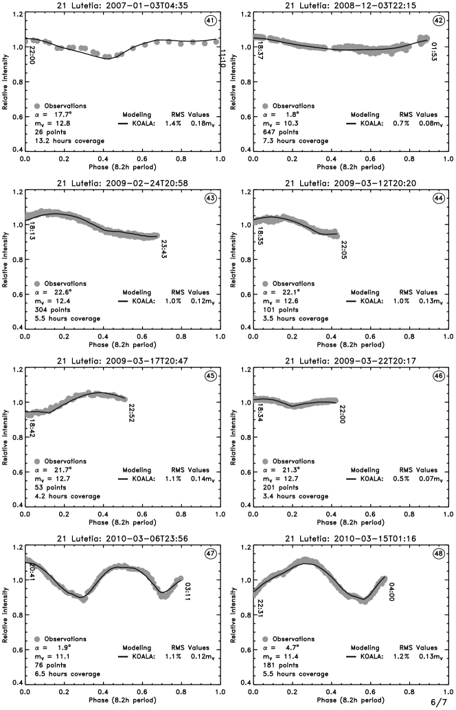
(f) Sixth set of lightcurves (2007-2010)

(f) Seventh set of lightcurves (2010)

Table 2: Characteristics of the pole solution obtained with KOALA. The pole solution is in agreement with the purely triaxial-ellipsoid results (7° of arc difference) presented by Drummond et al. [2010]. We list both $W_{0}$ and $t_{0}$ to orient the shape model in space at any time from the IAU definition [see Seidelmann et al. 2007] or the definition usually used in inversion techniques [following Kaasalainen et al. 2001]

$P_{s}$	ECJ2000	EQJ2000	$W_{0}$	$t_{0}$
(h)	($\lambda_{0}$,$\beta_{0}$ in °)	($\alpha_{0}$, $\delta_{0}$ in °)	(°)	(JD)
8.168 270 $\pm$ 0.000 001	(52,-6) $\pm$ 5	(52,12) $\pm$ 5	94 $\pm$ 2	2444822.35116

4 Rosetta flyby of (21) Lutetia

Finally, we investigate the regions of Lutetia that will be observed by Rosetta during the upcoming flyby on 2010 July 10. We used the shape model and spin solution described in section 3 and the spacecraft trajectory (obtained using the most recent spice kernels) to derive the relative position (SPK) and orientation (PCK) of Rosetta and Lutetia. This provides the relative distance between Rosetta and (21) Lutetia, the coordinates of the Sub-Rosetta Point (SRP) and Sub-Solar Point (SSP), the illuminated fraction of Lutetia surface, and the Solar phase angle as function of time.
At the time of the flyby, the northern hemisphere will be in constant sunlight (SSP_β will be +52°), while regions below -35° latitude will be in a constant shadow (see Table 3 and Fig. 5). Therefore, extreme southern latitudes of Lutetia will not be observable from Rosetta in optical wavelengths, preventing precise shape reconstruction of the southern regions. Therefore, size determination along the rotation axis will probably have to rely on thermal observations conducted with MIRO [Gulkis et al. 2007] (the observation plan for the flyby includes a slew along the shadowed regions of the asteroid).
Rosetta will approach Lutetia with a SRP_β close to +48°, and a nearly constant phase angle of $\sim$10°, observing Lutetia as it rotates around its spin axis. The solar phase angle will then decrease slowly while SRP_β will increase. The lowest solar phase angle (0.7°) will occur at 1040 seconds (17min) before closest approach (CA). A few minutes before CA, the spacecraft will fly over the North pole at a maximum latitude of about +84°, allowing the putative large-scale depression reported here to be observed. CA will then occur at 79° phase angle over +48° latitude, close to the terminator. At that time, the relative speed between Rosetta and Lutetia will be about 15 km/s and the distance will reach its minimum at 3063 km. This implies an apparent size of Lutetia of about 2 degrees at CA, which corresponds approximately to the field of view of the Narrow Angle Camera (NAC) of the OSIRIS instrument [Keller et al. 2007].
The SRP will then move rapidly into the Southern hemisphere. A few tens of seconds after CA, the day-to-night thermal transition will be observed between latitudes +30° and +40°, over 280° longitude, at rapidly increasing phase angles. One hour after CA, the SRP will finally enter into the “seasonal” shadow area between -20° and -40° latitude, at very high phase angles ($\geq 150$°). Differences in the thermal emissions coming from both regions (night and winter) should be detectable with MIRO [Gulkis et al. 2007]. The distance will then increase rapidly while the phase angle will reach an almost constant value of about 170°.

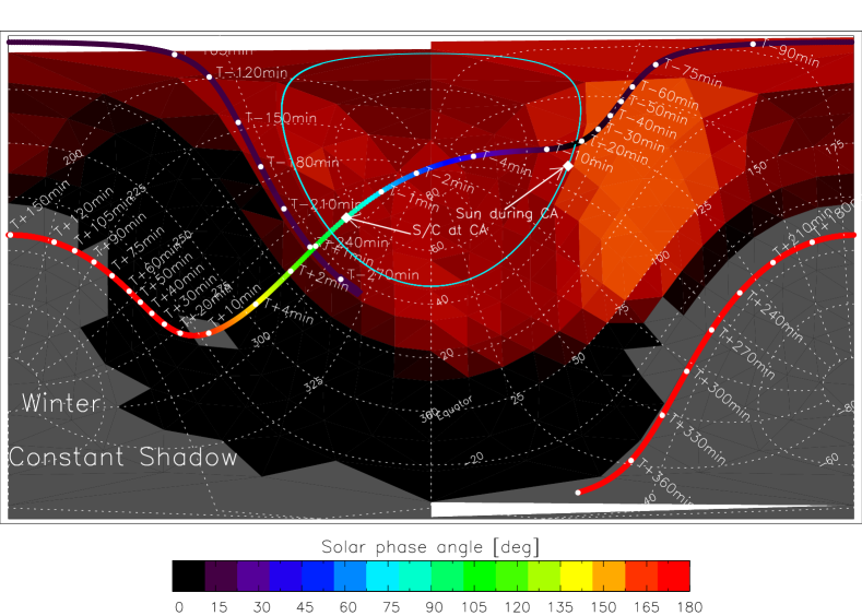
Figure 5: Oblique Mercator projection of the Sub-Rosetta Point (SRP) and Sub-Solar Point (SSP) paths during the Lutetia encounter on 2010 July 10 by the Rosetta spacecraft. The grey area near the South pole represents surface points where the Sun is never above the local horizon at the encounter epoch (constant shadow area). The reddish shades on the surface give the local illumination conditions at closest approach (CA), with the equatorial black band corresponding to night time at CA. Brighter shades of red depict a smaller local solar incidence angle (Sun high in sky), while darker shades represent a larger solar incidence angle. For flyby imaging, crater measurements will be much better in regions of low sun (high incidence angle), while albedo/color will be better discernible at high sun. The thin blue line is the SSP path, with the Sun traversing this path east-to-west on Lutetia’s surface. The location of the SRP with time (thick, multi-colored line) is color-coded in phase angle (see Table 3 for a detailed listing of the path coordinates as a function of time). Positions of the SSP and SRP at CA are labeled for convenience. The actual estimate of the CA time is 15:44 UT, but it may vary by a few tens of seconds, depending on trajectory-correction maneuvers that are applied to the spacecraft before the encounter. Thus, we provide times relative to CA, indicated in minutes.

Table 3: Sub-Rosetta Point (SRP) coordinates (longitude $\lambda$, latitude $\beta$), Sub-Solar Point (SSP) coordinates and phase angle ($\alpha$) as a function of the nominal flyby schedule (UT time $t$) and relatively to the instant of Closest Approach (CA), listed in bold.

Time $t$	$t$-CA	Distance	SRPλ	SRPβ	SSPλ	SSPβ	$\alpha$
(UT)	(min)	(km)	(°)	(°)	(°)	(°)	(°)
11:14:35	-270	242 906	309.5	36.2	310.1	46.6	10.4
11:44:35	-240	215 918	287.5	36.3	288.1	46.6	10.3
12:14:35	-210	188 930	265.4	36.5	266.0	46.6	10.2
12:44:35	-180	161 941	243.4	36.6	244.0	46.6	10.0
13:14:35	-150	134 953	221.4	36.8	221.9	46.6	9.8
13:44:35	-120	107 968	199.3	37.2	199.9	46.6	9.5
13:59:35	-105	94 477	188.3	37.4	188.9	46.6	9.2
14:14:35	-90	80 990	177.3	37.7	177.9	46.6	8.9
14:29:35	-75	67 506	166.3	38.1	166.9	46.6	8.5
14:44:35	-60	54 028	155.3	38.8	155.8	46.6	7.9
14:54:35	-50	45 049	148.0	39.4	148.5	46.6	7.2
15:04:35	-40	36 079	140.7	40.4	141.1	46.6	6.2
15:14:35	-30	27 126	133.4	42.0	133.8	46.6	4.6
15:24:35	-20	18 216	126.1	45.2	126.5	46.6	1.5
15:34:35	-10	9 468	119.1	54.3	119.1	46.6	7.7
15:40:35	-4	4 689	116.9	75.8	114.7	46.6	29.2
15:42:35	-2	3 513	282.3	85.0	113.2	46.6	48.3
15:43:35	-1	3 150	288.8	71.0	112.5	46.6	62.3
15:44:35	CA	3 016	289.4	54.7	111.8	46.6	78.7
15:45:35	1	3 140	289.2	38.3	111.0	46.6	95.1
15:46:35	2	3 496	288.7	24.2	110.3	46.6	109.2
15:48:35	4	4 666	287.5	5.0	108.8	46.6	128.4
15:54:35	10	9 443	283.5	-16.7	104.4	46.6	150.1
16:04:35	20	18 192	276.3	-25.9	97.1	46.6	159.2
16:14:35	30	27 104	269.0	-29.1	89.7	46.6	162.4
16:24:35	40	36 058	261.7	-30.7	82.4	46.6	164.0
16:34:35	50	45 029	254.4	-31.6	75.0	46.6	165.0
16:44:35	60	54 009	247.0	-32.3	67.7	46.6	165.6
16:59:35	75	67 486	236.0	-32.9	56.7	46.6	166.3
17:14:35	90	80 969	225.0	-33.4	45.6	46.6	166.7
17:29:35	105	94 455	214.0	-33.7	34.6	46.6	167.0
17:44:35	120	107 944	203.0	-33.9	23.6	46.7	167.2
18:14:35	150	134 925	181.0	-34.2	1.6	46.7	167.6
18:44:35	180	161 912	158.9	-34.4	339.5	46.7	167.8
19:14:35	210	188 903	136.9	-34.6	317.5	46.7	167.9
19:44:35	240	215 894	114.9	-34.7	295.5	46.7	168.0
20:14:35	270	242 885	92.8	-34.8	273.4	46.7	168.1
20:44:35	300	269 874	70.8	-34.9	251.4	46.7	168.2
21:14:35	330	296 862	48.7	-34.9	229.3	46.7	168.2
21:44:35	360	323 849	26.7	-35.0	207.3	46.7	168.3

5 Conclusions

We have reported disk-resolved imaging observations of (21) Lutetia obtained with the W. M. Keck and Very Large Telescope observatories in 2007, 2008, and 2009. We have derived the shape and spin of (21) Lutetia using the Knitted Occultation, Adaptive-optics, and Lightcurve Analysis (KOALA) method, which is based on combining these AO images with optical lightcurves gathered from over four decades.
The shape of (21) Lutetia is well described by a Camembert wedge, and our shape model suggests the presence of several concavities near its north pole and around its equator. The spin axis of Lutetia is tilted with respect to its orbital plane, much like Uranus, implying strong seasonal effects on its surface. At the time of the Rosetta flyby, (21) Lutetia’s northern hemisphere will be illuminated while the southern hemisphere will be in long-term darkness, hindering the size determination from Rosetta.
The next opportunity to observe Lutetia’s shortest dimension, impacting its volume determination, will occur in 2011 July, one year after Rosetta flyby, when the sub-Earth point will be close to its equator (SEP_β of +31°). During this time, observations using large telescopes equipped with adaptive-optics will allow refinement of Lutetia’s short dimension and thus improve the volume determination. This ground-based support will be essential to take advantage of the high-precision mass determination provided by the spacecraft deflection observed during the flyby.

References

- Barucci et al. (2008) Barucci, M. A., Fornasier, S., Dotto, E., et al. 2008, Astronomy and Astrophysics, 477, 665
- Barucci et al. (2005) Barucci, M. A., Fulchignoni, M., Fornasier, S., et al. 2005, Astronomy and Astrophysics, 430, 313
- Barucci et al. (2007) Barucci, M. A., Fulchignoni, M., & Rossi, A. 2007, Space Science Reviews, 128, 67
- Behrend et al. (2006) Behrend, R., Bernasconi, L., Roy, R., et al. 2006, Astronomy and Astrophysics, 446, 1177
- Belskaya et al. (2010) Belskaya, I. N., Fornasier, S., Krugly, Y. N., et al. 2010, submitted to Astronomy and Astrophysics
- Belskaya & Lagerkvist (1996) Belskaya, I. N. & Lagerkvist, C.-I. 1996, Planetary and Space Science, 44, 783
- Birlan et al. (2006) Birlan, M., Vernazza, P., Fulchignoni, M., et al. 2006, Astronomy and Astrophysics, 454, 677
- Bottke et al. (2002) Bottke, Jr., W. F., Cellino, A., Paolicchi, P., & Binzel, R. P. 2002, Asteroids III, 3
- Bowell et al. (1978) Bowell, E., Chapman, C. R., Gradie, J. C., Morrison, D., & Zellner, B. H. 1978, Icarus, 35, 313
- Carry et al. (2008) Carry, B., Dumas, C., Fulchignoni, M., et al. 2008, Astronomy and Astrophysics, 478, 235
- Carry et al. (2010) Carry, B., Dumas, C., Kaasalainen, M., et al. 2010, Icarus, 205, 460
- Carvano et al. (2008) Carvano, J. M., Barucci, M. A., Delbò, M., et al. 2008, Astronomy and Astrophysics, 479, 241
- Chang & Chang (1963) Chang, Y. C. & Chang, C. S. 1963, Acta Astronautica Sinica, 11, 139
- Chapman et al. (1975) Chapman, C. R., Morrison, D., & Zellner, B. H. 1975, Icarus, 25, 104
- Conan et al. (2000) Conan, J.-M., Fusco, T., Mugnier, L. M., & Marchis, F. 2000, The Messenger, 99, 38
- Conrad et al. (2007) Conrad, A. R., Dumas, C., Merline, W. J., et al. 2007, Icarus, 191, 616
- DeMeo et al. (2009) DeMeo, F. E., Binzel, R. P., Slivan, S. M., & Bus, S. J. 2009, Icarus, 202, 160
- Denchev (2000) Denchev, P. 2000, Planetary and Space Science, 48, 987
- Denchev et al. (1998) Denchev, P., Magnusson, P., & Donchev, Z. 1998, Planetary and Space Science, 46, 673
- Dotto et al. (1992) Dotto, E., Barucci, M. A., Fulchignoni, M., et al. 1992, Astronomy and Astrophysics Supplement Series, 95, 195
- Drummond (2000) Drummond, J. D. 2000, in Laser Guide Star Adaptive Optics for Astronomy, ed. N. Ageorges & C. Dainty, 243–262
- Drummond et al. (2009) Drummond, J. D., Christou, J. C., & Nelson, J. 2009, Icarus, 202, 147
- Drummond et al. (2010) Drummond, J. D., Conrad, A. R., Merline, W. J., et al. 2010, submitted to Astronomy and Astrophysics
- Dunham & Herald (2009) Dunham, D. W. & Herald, D. 2009, Asteroid Occultations V7.0. EAR-A-3-RDR-OCCULTATIONS-V7.0., NASA Planetary Data System
- Faury et al. (2009) Faury, G., Jorda, L., Lamy, P. L., et al. 2009, in Bulletin of the American Astronomical Society, Vol. 41, Bulletin of the American Astronomical Society, 559
- Gulkis et al. (2007) Gulkis, S., Frerking, M., Crovisier, J., et al. 2007, Space Science Reviews, 128, 561
- Kaasalainen (2010) Kaasalainen, M. 2010, ArXiv e-prints, Inverse Problems and Imaging, in press
- Kaasalainen & Torppa (2001) Kaasalainen, M. & Torppa, J. 2001, Icarus, 153, 24
- Kaasalainen et al. (2001) Kaasalainen, M., Torppa, J., & Muinonen, K. 2001, Icarus, 153, 37
- Kaasalainen et al. (2002) Kaasalainen, M., Torppa, J., & Piironen, J. 2002, Astronomy and Astrophysics, 383, L19
- Keller et al. (2007) Keller, H. U., Barbieri, C., Lamy, P. L., et al. 2007, Space Science Reviews, 128, 433
- Kryszczyńska et al. (2007) Kryszczyńska, A., La Spina, A., Paolicchi, P., et al. 2007, Icarus, 192, 223
- Lagerkvist et al. (1995) Lagerkvist, C.-I., Erikson, A., Debehogne, H., et al. 1995, Astronomy and Astrophysics Supplement Series, 113, 115
- Lazzarin et al. (2010) Lazzarin, M., Magrin, S., Marchi, S., et al. 2010, submitted to MNRAS
- Lazzarin et al. (2004) Lazzarin, M., Marchi, S., Magrin, S., & Barbieri, C. 2004, Astronomy and Astrophysics, 425, L25
- Lazzarin et al. (2009) Lazzarin, M., Marchi, S., Moroz, L. V., & Magrin, S. 2009, Astronomy and Astrophysics, 498, 307
- Lenzen et al. (2003) Lenzen, R., Hartung, M., Brandner, W., et al. 2003, SPIE, 4841, 944
- Lupishko & Belskaya (1989) Lupishko, D. F. & Belskaya, I. N. 1989, Icarus, 78, 395
- Lupishko et al. (1983) Lupishko, D. F., Belskaya, I. N., & Tupieva, F. A. 1983, Soviet Astronomy Letters, 9, 358
- Lupishko & Velichko (1987) Lupishko, D. F. & Velichko, F. P. 1987, Kinematika i Fizika Nebesnykh Tel, 3, 57
- Lupishko et al. (1987) Lupishko, D. F., Velichko, F. P., Bel’Skaia, I. N., & Shevchenko, V. G. 1987, Kinematika i Fizika Nebesnykh Tel, 3, 36
- Magri et al. (1999) Magri, C., Ostro, S. J., Rosema, K. D., et al. 1999, Icarus, 140, 379
- Magri et al. (2007) Magri, C., Ostro, S. J., Scheeres, D. J., et al. 2007, Icarus, 186, 152
- Marchis et al. (2002) Marchis, F., de Pater, I., Davies, A. G., et al. 2002, Icarus, 160, 124
- McCord & Chapman (1975) McCord, T. B. & Chapman, C. R. 1975, Astrophysical Journal, 195, 553
- Morrison (1977) Morrison, D. 1977, Icarus, 31, 185
- Mueller et al. (2006) Mueller, M., Harris, A. W., Bus, S. J., et al. 2006, Astronomy and Astrophysics, 447, 1153
- Mugnier et al. (2004) Mugnier, L. M., Fusco, T., & Conan, J.-M. 2004, Journal of the Optical Society of America A, 21, 1841
- Nedelcu et al. (2007) Nedelcu, D. A., Birlan, M., Vernazza, P., et al. 2007, Astronomy and Astrophysics, 470, 1157
- Perna et al. (2007) Perna, D., Dotto, E., De Luise, F., et al. 2007, in Bulletin of the American Astronomical Society, Vol. 38, Bulletin of the American Astronomical Society, 448
- Perna et al. (2010) Perna, D., Dotto, E., Lazzarin, M., et al. 2010, Astronomy and Astrophysics, 513, L4
- Rivkin et al. (1995) Rivkin, A. S., Howell, E. S., Britt, D. T., et al. 1995, Icarus, 117, 90
- Rivkin et al. (2000) Rivkin, A. S., Howell, E. S., Lebofsky, L. A., Clark, B. E., & Britt, D. T. 2000, Icarus, 145, 351
- Rousset et al. (2003) Rousset, G., Lacombe, F., Puget, P., et al. 2003, SPIE, 4839, 140
- Schulz et al. (2009) Schulz, R., Accomazzo, A., Küppers, M., Schwehm, G., & Wirth, K. 2009, in Bulletin of the American Astronomical Society, Vol. 41, Bulletin of the American Astronomical Society, 563
- Seidelmann et al. (2007) Seidelmann, P. K., Archinal, B. A., A’Hearn, M. F., et al. 2007, Celestial Mechanics and Dynamical Astronomy, 98, 155
- Shepard et al. (2008) Shepard, M. K., Clark, B. E., Nolan, M. C., et al. 2008, Icarus, 195, 184
- Tedesco et al. (2002) Tedesco, E. F., Noah, P. V., Noah, M. C., & Price, S. D. 2002, Astronomical Journal, 123, 1056
- Tedesco et al. (2004) Tedesco, E. F., Noah, P. V., Noah, M. C., & Price, S. D. 2004, IRAS-A-FPA-3-RDR-IMPS-V6.0, NASA Planetary Data System
- Torppa et al. (2003) Torppa, J., Kaasalainen, M., Michalowski, T., et al. 2003, Icarus, 164, 346
- van Dam et al. (2007) van Dam, M. A., Johansson, E. M., Stomski Jr., P. J., et al. 2007, Performance of the Keck II AO system
- van Dam et al. (2004) van Dam, M. A., Le Mignant, D., & Macintosh, B. 2004, Applied Optics, 43, 5458
- Vernazza et al. (2009) Vernazza, P., Brunetto, R., Binzel, R. P., et al. 2009, Icarus, 202, 477
- Weaver et al. (2009) Weaver, H. A., Feldman, P. D., Merline, W. J., et al. 2009, ArXiv e-prints
- Witasse et al. (2006) Witasse, O., Lebreton, J.-P., Bird, M. K., et al. 2006, Journal of Geophysical Research (Planets), 111, 7
- Zappala et al. (1984) Zappala, V., di Martino, M., Knezevic, Z., & Djurasevic, G. 1984, Astronomy and Astrophysics, 130, 208
- Zellner & Gradie (1976) Zellner, B. H. & Gradie, J. C. 1976, Astronomical Journal, 81, 262