The Bianchi Variety

Abstract

The totality $\mathrm{Lie\,}(V)$ of all Lie algebra structures on a vector space $V$ over a field $\mathbb{F}$ is an algebraic variety over $\mathbb{F}$ on which the group $\mathrm{GL\,}(V)$ acts naturally. We give an explicit description of $\mathrm{Lie\,}(V)$ for $\dim V=3$ which is based on the notion of compatibility of Lie algebra structures.

Keywords: Lie Algebra, Poisson Geometry, Commutative Algebra, Cohomology of Lie Algebras, Moduli Space, Deformation.

MSC Classification: 13D10, 14D99, 17B99, 53D99.

Introduction

Historical remarks

The problem of classifying 3–dimensional Lie algebras over $\mathbb{R}$ was firstly solved by L. Bianchi at the end of the eigtheen century. Recently, various works concerning classifications of low–dimensional Lie algebras appeared (see, for instance, [6] for a list of 4–dimensional Lie algebras and [7] for a special list of real Lie algebras of dimension $\leq 8$). Now Bianchi classification can be obtained in a more elegant coordinate–free manner. For instance, in [4] this is done on the basis of the invariants of Lie structures, in [2] the co–differential graded calculus is used, in [2] the outer derivations, etc. A shortcoming of the original Bianchi method, as well as of the above–cited works, is that they do not allow a satisfactory description of deformations of 3–dimensional Lie algebras (see [2, 3, 8] and references therein).

It should be especially stressed the recently emerged important role of Poisson geometry in various questions related with Lie algebras and, first of all, classification, representation, deformations, etc. (see [6], [13] and [9]). We shall exploit it throughout the paper.

Aim of the paper

Let $V$ be a vector space over field $\mathbb{F}$ of characteristic different from 2. All Lie algebra structures on $V$ form an algebraic variety denoted by $\mathrm{Lie\,}(V)$. We call it “the Bianchi variety” if $\dim V=3$. The aim of this paper is to describe the Bianchi variety in a geometrically transparent manner.

Our approach is based on the notion of compatibility of Lie structures (see, for instance, [13]) and differential calculus over the “manifold” $V^{*}$ in the spirit of [1]. First we show that all three–dimensional unimodular Lie algebra structures form an algebraic variety $\mathrm{Lie\,}_{0}(V)$ which is naturally identified with the space of symmetric bilinear forms on $V^{*}$. Recall that a Lie algebra is unimodular if operators of its adjoint representation are traceless. Then we show that a generic Lie structure can be obtained by adding a non–unimodular “charge” to a unimodular structure. This “charge” (see pag. 12) is a particular non–unimodular structure, which reduces the problem to a description of how such a “charge” can be attached to unimodular structures.

The obtained description of $\mathrm{Lie\,}(V)$ allows, besides others, to see directly peculiarities of deformations of 3–dimensionale Lie structures. Also from this point of view the Bianchi classification can be seen as moduli space $\frac{\mathrm{Lie\,}(V)}{\mathrm{GL\,}(V)}$.

Notations and preliminaries

We shall use the Einstein summation convention, assuming that the index “$i$” in $\frac{\partial}{\partial x_{i}}$ is treated as an upper one.

By a Lie structure on a vector space $V$ we mean a skew–symmetric $\mathbb{F}$–bracket $[\,\cdot\,,\,\cdot\,]$ on $V$, which fulfills the Jacobi Identity

$$[v,[w,z]]=[[v,w],z]+[w,[v,z]]\quad\forall v,w,z\in V.$$

Fix a basis $\{x_{1},x_{2},\ldots,x_{n}\}$ of $V$. This induces a basis $\{\xi^{1},\xi^{2},\ldots,\xi^{n}\}$ of $V^{*}$, a volume $n$–covector $\boldsymbol{\xi}\stackrel{{\scriptstyle\mathrm{def}}}{{=}}\xi^{1}\wedge\xi^{2}\wedge\cdots\wedge\xi^{n}$, and its dual $\boldsymbol{v}$.

An element $c$ of $V\otimes_{\mathbb{F}}\bigwedge^{2}(V^{*})$ looks as $c=c^{k}_{ij}x_{k}\otimes\xi^{i}\wedge\xi^{j}$ and defines a Lie algebra structure iff

$$c_{aj}^{k}c_{bc}^{j}+c_{cj}^{k}c_{ab}^{j}+c_{bj}^{k}c_{ca}^{j}=0,\quad a,b,c,k=1,2,\ldots,n.$$ (1)

This way $\mathrm{Lie\,}(V)$ is identified with the affine algebraic variety in $V\otimes_{\mathbb{F}}\bigwedge^{2}(V^{*})$ determined by equations (1), and a Lie structure $c$ identifies with the family of its structure constants $\{c_{ij}^{k}\}$. Obviously, a natural action of $\mathrm{GL\,}(V)$ on $V\otimes_{\mathbb{F}}\bigwedge^{2}(V^{*})$ leaves $\mathrm{Lie\,}(V)$ invariant, and defines an action of $\mathrm{GL\,}(V)$ on $\mathrm{Lie\,}(V)$.

If $\dim V=3$, we introduce the basis $\{\boldsymbol{\xi}^{h}\}_{h=1,2,3}$ of $\bigwedge^{2}(V^{*})$, $\boldsymbol{\xi}^{h}\stackrel{{\scriptstyle\mathrm{def}}}{{=}}\epsilon^{h}_{\ ij}\xi^{i}\wedge\xi^{j}$, where $\epsilon_{\ ij}^{h}$ is purely skew–symmetric symbol. Then an element $c$ of $V\otimes_{\mathbb{F}}\bigwedge^{2}(V^{*})$ looks as $c=c_{h}^{k}x_{k}\otimes\boldsymbol{\xi}^{h}$, where $c_{ij}^{k}=c_{h}^{k}\epsilon_{\ ij}^{h}$, and (1) becomes

$$\sum_{i}\epsilon_{mi}^{h}c_{i}^{m}c_{h}^{k}=0,\quad k=1,2,3.$$ (2)

1 Differential Calculus over algebra $S(V)$

In this section elements of differential calculus over $V^{*}$ are sketched, in the the spirit of differential calculus over commutative algebras (see [1]). Below $V$ stands for e a finite–dimensional $\mathbb{F}$–vector space, $n=\dim V$, and $S(V)=\bigoplus S_{i}(V)$, where $S_{i}(V)$ is the $i$–th symmetric power of $V$. The algebra $S(V)$ is naturally interpreted as the algebra of polynomials on $V^{*}$, whose $\mathbb{F}$–spectrum identifies with $V^{*}$. Consequently, the necessary elements of differential calculus on the “manifold” $V^{*}$ are interpreted as those over commutative algebra $S(V)$.

Denote by $D(V^{*})$ the $S(V)$–module of derivations of the algebra $S(V)$, which we interpret as vector fields on $V^{*}$. Then, obviously, the map

$$D(V^{*}) \longrightarrow S(V)\otimes_{\mathbb{F}}V^{*}$$ (3)

$$X \leftrightarrow X|_{V}$$

$$X_{\theta}=a_{i_{1},\dots,i_{n},i}x_{1}^{i_{1}}\cdots x_{n}^{i_{n}}\frac{\partial}{\partial x_{i}} \leftrightarrow a_{i_{1},\ldots,i_{n},i}x_{1}^{i_{1}}\cdots x_{n}^{i_{n}}\otimes\xi^{i}=\theta$$

where $\frac{\partial}{\partial x_{i}}(v_{1}v_{2}\cdots v_{m})\stackrel{{\scriptstyle\mathrm{def}}}{{=}}\sum_{i=1}^{n}\xi^{i}(v)v_{1}\cdots v_{i-1}v_{i}\cdots v_{m}$, is a $S(V)$–module isomorphism. Put

$$D_{\bullet}(V^{*})\stackrel{{\scriptstyle\mathrm{def}}}{{=}}\bigoplus_{i}D_{i}(V^{*}),$$ (4)

where $D_{i}(V^{*})$ is the $S(V)$–module of skew–symmetric multi–$i$–derivations of the algebra $S(V)$, which we interpret as $i$–vector fields on $V^{*}$. Then a similar isomorphism between $D_{\bullet}(V^{*})$ and $S(V)\otimes_{\mathbb{F}}\bigwedge^{\bullet}V^{*}$ holds. In particular, $c=c_{{ij}}^{k}x_{k}\otimes\xi^{i}\wedge\xi^{j}$ corresponds to the bi–vector field

$${P^{c}}\stackrel{{\scriptstyle\mathrm{def}}}{{=}}c_{ij}^{k}x_{k}\frac{\partial}{\partial x_{i}}\wedge\frac{\partial}{\partial x_{j}}.$$ (5)

If $n=3$ and $c=c_{h}^{k}x_{k}\otimes\boldsymbol{\xi}^{h}$, (5) reads

$${P^{c}}\stackrel{{\scriptstyle\mathrm{def}}}{{=}}c_{h}^{k}\epsilon_{ij}^{h}x_{k}\frac{\partial}{\partial x_{i}}\wedge\frac{\partial}{\partial x_{j}}.$$ (6)

The algebra $S(V)\otimes_{\mathbb{F}}\bigwedge^{\bullet}(V^{*})$ is $\mathbb{Z}_{2}$–graded. For example, linear vector fields are exactly elements of bidegree $(1,1)$. We emphasize that accordingly to (3) linear vector fields correspond to endomorphisms of vector space $V$,

$${X_{\varphi}}\stackrel{{\scriptstyle\mathrm{def}}}{{=}}\varphi_{i}^{j}x_{j}\frac{\partial}{\partial x_{i}},$$ (7)

where, by definition, $X_{\varphi}(v)=\varphi(v)$, $v\in V$.

The Liouville vector field on $V^{*}$

$$X_{\mathrm{id}}=x^{i}\frac{\partial}{\partial x^{i}}$$

plays a special role, and is denoted by $\Delta$. A bi–vector is called linear when its bidegree is $(1,2)$, quadratic if it is $(2,2)$, etc. These definitions extend straightforwardly to all tensor fields over $V^{*}$.

Similarly,

$$\Lambda^{\bullet}(V^{*})\stackrel{{\scriptstyle\mathrm{def}}}{{=}}\bigoplus_{i}\Lambda^{i}(V^{*}),$$ (8)

is the $S(V)$–module of polynomial differential forms on $V^{*}$. Here the $S(V)$–module $\Lambda^{i}(V^{*})$ of $i$–th order differential forms on $V^{*}$ is identified with the $i$–th skew–symmetric power $\bigwedge^{i}(S(V)\otimes_{\mathbb{F}}V)$ of the $S(V)$–module $S(V)\otimes_{\mathbb{F}}V$, which coincides with $S(V)\otimes_{\mathbb{F}}\bigwedge^{\bullet}(V)$. In particular, this identification for $i=1$ looks as

$$\Lambda^{1}(V^{*}) \longrightarrow S(V)\otimes_{\mathbb{F}}V$$ (9)

$$\omega_{q}=a^{i}_{i_{1},\ldots,i_{n}}x_{1}^{i_{1}}\cdots x_{n}^{i_{n}}dx_{i} \leftrightarrow a^{i}_{i_{1},\dots,i_{n}}x_{1}^{i_{1}}\cdots x_{n}^{i_{n}}\otimes x_{i}=q.$$

In view of the above isomorphisms, natural operations with multi–vector fields and differential forms, such as insertion, Lie derivative, Schouten bracket, etc., are easily reproduced in $S(V)\otimes_{\mathbb{F}}\bigwedge^{\bullet}(V^{*})$ and $S(V)\otimes_{\mathbb{F}}\bigwedge^{\bullet}(V)$. These algebras are naturally bi–graded ($\mathbb{Z}^{2}$–graded). The total degree of an element of bidegree $(p,q)$ is $p+q$. Obviously, a tensor field $T$ is homogeneous of total degree $k$ iff $L_{\Delta}(T)=kT$. The Schouten bracket is denoted by $[[\cdot,\cdot]]$.

Elements of $S(V)\otimes_{\mathbb{F}}V^{*}\subset S(V)\otimes_{\mathbb{F}}\bigwedge^{\bullet}(V^{*})$ (resp., $S(V)\otimes_{\mathbb{F}}V\subset S(V)\otimes_{\mathbb{F}}\bigwedge^{\bullet}(V)$) will be called linear. A linear 1–form ${\omega_{q}}\stackrel{{\scriptstyle\mathrm{def}}}{{=}}q^{ij}x_{i}dx_{j}$, is closed iff the matrix $q=\|q^{ij}\|$ is symmetric. Also, observe that if $n=3$ and $q$ is skew–symmetric then $\omega_{q}\wedge d\omega_{q}$ is zero.

A bivector $P\in S(V)\otimes_{\mathbb{F}}\bigwedge^{2}(V^{*})$ is called Poisson if $[[P,P]]=0$. The following fundamental correspondence, for the first time established by S. Lie, is the starting point of the paper.

Proposition 1.

There is a one–to–one correspondence between Lie algebra structures on $V$ and linear Poisson bivectors on $V^{*}$. Namely,

$$c\equiv\{c_{ij}^{k}\}\leftrightarrow P^{c}=c_{ij}^{k}x_{k}\frac{\partial}{\partial x_{i}}\wedge\frac{\partial}{\partial x_{j}}.$$ (10)

$P^{c}$ given by (5) is called the Poisson bi–vector associated with $c$, and the corresponding to it bracket is referred to as the Lie–Poission bracket on $S(V)$ (see [6]).

Recall (see[12]) that the map

$$d_{P}\stackrel{{\scriptstyle\mathrm{def}}}{{=}}[[P,\,\cdot\,]]:D_{\bullet}(V^{*})\longmapsto D_{\bullet}(V^{*}),\quad P\in D_{2}(V^{*})$$ (11)

is a differential in $D(V^{*})$, i.e., $d_{P}^{2}=0$, iff $P$ is a Poisson bivector. Moreover we have (see [12])

Proposition 2.

There exists an unique homomorphism $\Gamma_{P}:D_{\bullet}(V^{*})\longrightarrow\Lambda^{\bullet}(V^{*})$ of $S(V)$–algebras which is a cochain map from $(D_{\bullet}(V^{*}),d_{P})$ to $(\Lambda^{\bullet}(V^{*}),d)$.

1–cocycles (resp., 1–coboundaries) of $d_{P}$ are called canonical (resp., Hamiltonian) vector fields on $V^{*}$ (with respect to the Poisson structure $P$ on $V^{*}$). The Hamiltonian vector field corresponding to the Hamiltonian function $f\in S(V)$ will be denoted by $P_{f}$, i.e., $P_{f}=d_{P}(f)$. It is easy to see that $P_{f}=-i_{df}(P)$ (the contraction of $df$ and $P$).

When $P=P_{c}$, the corresponding to the Hamiltonian vector fields foliation is referred to as the symplectic foliation determined by $c$.

From now on we shall assume that $\dim V=3$. The volume form $\boldsymbol{v}=dx^{1}\wedge dx^{2}\wedge dx^{3}$ determines a standard duality between $i$–vector fields and $(3-i)$–differential forms. The linear bi–vector $P^{c}$ defined by (6) is dual to the linear 1–form

$$\alpha_{c}=\sum_{h}c_{{h}}^{k}x_{k}dx_{h},$$

i.e., $P^{c}(f,g)\boldsymbol{v}=df\wedge dg\wedge\alpha_{c}$, $f,g\in S(V)$.

We have (see[13])

Lemma 1.

$P\in D_{2}(V^{*})$ is Poisson iff $\alpha\wedge d\alpha=0$ for the dual to $P$ 1–form $\alpha$.

Denote by $q_{c}$ the bilinear form on $V^{*}$ corresponding to $\alpha_{c}$ in (9).

Corollary 1.

If $q_{c}$ is either symmetric, or skew–symmetric, then $c$ is a a Lie structure on $V$.

Proof.

Directly from Lemma 1 and Proposition 1. ∎

Hence $\mathrm{Lie\,}(V)$ can be identified with a subset in the space of linear differential 1–forms. As such, it contains the subspace $\mathrm{Lie\,}_{0}(V)$ of differential forms which correspond to symmetric bilinear forms on $V$ in (9), and the subspace $N$ of those which correspond to skew–symmetric differential forms. Recall that a structure $c$ is unimodular if and only if $\alpha_{c}$ is symmetric (see[13]). Accordingly, elements of $\mathrm{Lie\,}_{0}(V)$ (resp., $N$) are called unimodular (resp., purely non–unimodular).

Since a bilinear form splits into the sum of a symmetric and a skew–symmetric part, a Lie structure $c$ on $V$ can be “disassembled” into the sum of an unimodular component with a purely non–unimodular one,

$$\alpha_{c}=dF+\alpha,\quad dF\in\mathrm{Lie\,}_{0}(V),\alpha\in N.$$ (12)

In terms of Lie structures, (12) reads $c=c_{F}+c_{\alpha}$, where $c_{F}$ (resp., $c_{\alpha}$) is the Lie structure corresponding to $dF$ (resp., $\alpha$), and in terms of brackets,

$$[v,w]=[v,w]_{0}+[v,w]_{1},\quad v,w\in V$$

where $[\,\cdot\,,\,\cdot\,]$ (resp., $[\,\cdot\,,\,\cdot\,]_{0}$, $[\,\cdot\,,\,\cdot\,]_{1}$) is the Lie bracket on $V$ corresponding to $c$ (resp., $c_{F}$, $c_{\alpha}$).

Recall the following

Definition 1.

Elements $c_{1},c_{2}\in\mathrm{Lie\,}(V)$ are said to be compatible if $c_{1}+c_{2}\in\mathrm{Lie\,}(V)$.

So, the unimodular part $c_{F}$ of $c$ and its purely non–unimodular part $c_{\alpha}$ are compatible.

Disassembling (12) can also be read as $\alpha_{c}=\pi_{0}(\alpha_{c})+\alpha$, where

$$V\otimes_{\mathbb{F}}{\textstyle\bigwedge^{2}(V^{*})}\stackrel{{\scriptstyle\pi_{0}}}{{\longrightarrow}}\mathrm{Lie\,}_{0}(V)$$ (13)

is the canonical projection of bilinear forms onto symmetric ones.

Remark 1.

The possibility to identify Lie structures as a bilinear forms is a peculiarity of the three–dimensional case only.

The compatibility condition of two Lie structures are, obviously, expressed in terms of their unimodular and purely non–unimodular part as follows.

Lemma 2.

Lie structures $c_{dF+\alpha}$ and $c_{dG+\beta}$ are compatible if and only if

$$[[c_{F},c_{\beta}]]+[[c_{G},c_{\alpha}]]=0,$$ (14)

or, equivalently,

$$dF\wedge\beta+dG\wedge\alpha=0.$$ (15)

The following fact is obvious as well.

Lemma 3.

Let $P$ and $Q$ be commuting bi–vectors, and $v,w\in V$, Then $[[vP,wQ]]=vP(w)\wedge Q-wQ(v)\wedge P$.

2 Finite and infinitesimal $\mathrm{GL\,}(V)$–actions

Fix an automorphism $\psi$$\in\mathrm{GL\,}(V)$. The adjoint to $\psi$ map is a diffeomorphism of $V^{*}$, which we still denote by $\psi$. Indeed, $\psi$, the diffeomorphism, corresponds (in the sense of [1]) to the algebra automorphism of $S(V)$ whose restriction to $V$ coincides with $\psi$, the automorphism.

Then the action of $\psi$ is naturally prolonged to differential forms and multi–vector fields on $V^{*}$, and, in view of isomorphisms (3) and (9), to the algebras $S(V)\otimes_{\mathbb{F}}\bigwedge^{\bullet}(V^{*})$ and $S(V)\otimes_{\mathbb{F}}\bigwedge^{\bullet}(V)$, respectively. We keep the same symbol $\psi$ for the prolonged automorphism, except for differential forms, when the pull-back $\psi^{*}$ is used.

An easy consequence of Lemma 1 is that the action of $\mathrm{GL\,}(V)$ on linear differential 1–forms restricts to $\mathrm{Lie\,}(V)$. In terms of Lie brackets this action reads

$$[v,w]^{\prime}\stackrel{{\scriptstyle\mathrm{def}}}{{=}}\psi^{-1}([\psi(v),\psi(w)]),\quad v,w\in V,$$

where $[\,\cdot\,,\,\cdot\,]$ (resp., $[\,\cdot\,,\,\cdot\,]^{\prime}$) corresponds to $\alpha_{c}$, (resp., $\psi^{*}(\alpha_{c})$). It is straightforward to verify that $P^{\psi(c)}=\psi(P^{c})$.

Remark 2.

The identification $\alpha_{c}\leftrightarrow P^{c}$ of linear 1–forms with linear bi–vector does not commute with actions of $\mathrm{GL\,}(V)$ on them. Namely, we have

$$\psi^{*}(\alpha_{c})\cdot\det\psi=\alpha_{\psi(c)},\quad\psi\in\mathrm{GL\,}(V).$$

Denote by $\mathrm{Stab\,}(c)\stackrel{{\scriptstyle\mathrm{def}}}{{=}}\{\psi\in\mathrm{GL\,}(V)\ |\ {\psi(c)=c}\}\subseteq\mathrm{GL\,}(V)$ the stabilizer of $c$.

An endomorphism $\varphi$$\in\mathrm{End\,}(V)$, i.e., a linear vector field on $V^{*}$ (see (7)), can be interpreted as an infinitesimal automorphism and, as such, it acts on tensor fields on $V^{*}$ by Lie derivation. On the other hand, the differential $d_{P^{c}}$ (see (11)) acts on $\varphi$ and produces $d_{P^{c}}(\varphi)$. It is easy to verify that $L_{X_{\varphi}}(\alpha_{c})=\alpha_{d_{P^{c}}(\varphi)}.$ The infinitesimal counterpart of the stabilizer is the symmetry Lie sub–algebra

$$\mathrm{sym\,}(c)\stackrel{{\scriptstyle\mathrm{def}}}{{=}}\{\varphi\in\mathrm{End\,}(V)\ |\ L_{X_{\varphi}}(c)=0\}\subseteq\mathrm{End\,}(V).$$

Remark 3.

Notice that $d_{P^{c}}(\varphi)$ is a linear bi–vector field on $V^{*}$, but not necessarily a Poisson one.

We conclude this section by collecting basic facts about the cohomology of Lie structures (see [14] for more details), which will be used to describe the orbits of the Bianchi variety.

A linear bi–vector field $P$ such that $d_{P^{c}}(P)=0$ is called a 2–cocyle of $c$. These cocycles form a subspace $Z^{2}(c)$ in $\mathrm{End\,}(V)$. A linear bi–vector field $P$ such that $P=d_{P^{c}}(\varphi)$, for some endomorphism $\varphi$, is called a 2–coboundary of $c$. The totality of 2–coboundaries is a subspace of $Z^{2}(c)$ denoted by $B^{2}(c)$. The quotient space $H^{2}(c)\stackrel{{\scriptstyle\mathrm{def}}}{{=}}\frac{Z^{2}(c)}{B^{2}(c)}$ is called the 2–cohomology of $c$.

Intuitively, the tangent space at $c$ to $\mathrm{Lie\,}(V)$ may be taught as the affine subspace parallel to $Z^{2}(c)$ and passing through $c$. Similarly, the tangent space at $c$ to $\mathrm{GL\,}(V)\cdot c$ may be viewed as the affine subspace parallel to $B^{2}(c)$ and passing through $c$. So, in “smooth” points of $\mathrm{Lie\,}(V)$, we can interpret $\dim Z^{2}(c)$ as the dimension of $\mathrm{Lie\,}(V)$ at $c$, $\dim B^{2}(c)$ as the dimension of the orbit of $c$, and the difference $\dim Z^{2}(c)-\dim B^{2}(c)=\dim H^{2}(c)$ as its co–dimension.

3 The Canonical Disassembling of a 3–Dimensional Lie Structure

Firstly observe that $\mathrm{GL\,}(V)$ preserves the fibers of the projection $\pi_{0}$ of $V\otimes_{\mathbb{F}}V$ over $\mathrm{Lie\,}_{0}(V)$.

Put $Z_{N}^{2}(dF)\stackrel{{\scriptstyle\mathrm{def}}}{{=}}Z^{2}(c_{F})\cap N$. The following assertion is a direct consequence of the above definitions.

Proposition 3.

In the above notation the following conditions are equivalent:

• $dF+\alpha$ corresponds to a Lie structure,

• $c_{F}$ and $c_{\alpha}$ are compatible,

• $[[c_{F},c_{\alpha}]]=0$,

• $dF\wedge\alpha=0$,

• $\alpha\in Z_{N}^{2}(dF)$.

An easy consequence of Proposition 3 is the following

Lemma 4.

$Z_{N}^{2}(dF)=\zeta^{-1}(c_{F})$, with $\zeta\stackrel{{\scriptstyle\mathrm{def}}}{{=}}\left.\left(\pi_{0}\right)\right|_{\mathrm{Lie\,}(V)}$.

Note that the map $\zeta$ is not of constant–rank. Namely, the dimension of $\zeta^{-1}(c_{F})$ depends on the rank of the polynomial $F$. It should be stressed that $\zeta^{-1}(c_{F})$ is naturally interpreted as a variety of purely non–unimodular structures compatible with $dF$. We shall show that its dimension equals $3-\mathrm{rank\,}(dF)$.

To this end, we compute the Schouten brackets between the basis elements $\{x_{i}dx_{j}\}_{i,j=1,2,3}$ of $\mathrm{Lie\,}_{0}(V)$ and the purely non–unimodular Lie structures $\alpha_{i}\stackrel{{\scriptstyle\mathrm{def}}}{{=}}\varepsilon_{i}^{\ i_{1}i_{2}}x_{i_{1}}dx_{i_{2}}$, i.e., the basis elements of $N$.

We usually write ${\textstyle\frac{1}{2}}d(x_{i}^{2})$ instead of $x_{i}dx_{i}$, $i=1,2,3$.

Proposition 4.

$$[[c_{{\textstyle\frac{1}{2}}d(x_{i}^{2})},c_{\alpha_{j}}]]=\left\{\begin{array}[]{ll}0&\textrm{ if }j\neq i,\\ 2x_{j}\boldsymbol{\xi}&\textrm{ otherwise;}\end{array}\right.\quad[[c_{{\textstyle\frac{}{}}dx_{i_{1}}x_{i_{2}}},c_{\alpha_{j}}]]=\left\{\begin{array}[]{ll}0&\textrm{ if }j\neq i_{1},i_{2},\\ 2x_{i_{1}}\boldsymbol{\xi}&\textrm{ if }j=i_{2},\\ 2x_{i_{2}}\boldsymbol{\xi}&\textrm{ if }j=i_{1}.\end{array}\right.$$

Proof.

From $d\alpha_{j}=\varepsilon_{j}^{\ i_{1}i_{2}}dx_{i_{1}}\wedge dx_{i_{2}}$ it follows that $dx_{i}^{2}\wedge\alpha_{j}=0$ when $j\neq i$ and $dx_{i_{1}}x_{i_{2}}\wedge\alpha_{j}=0$ when $j\neq i_{1},i_{2}$. Then, in view of Corollary 3, this gives the result for $i\neq j$ and for $i\neq i_{1},i_{2}$.

Next, by using Lemma 3 we have

$$[[c_{x_{1}dx_{1}},c_{x_{2}dx_{3}-x_{3}dx_{2}}]] =[[x_{1}\xi^{2}\wedge\xi^{3},x_{2}\xi^{1}\wedge\xi^{2}-x_{3}\xi^{3}\wedge\xi^{1}]]$$

$$={x_{1}\xi^{3}\wedge\xi^{1}\wedge\xi^{2}+x_{1}\xi^{2}\wedge\xi^{3}\wedge\xi^{1}}=2x_{1}\boldsymbol{\xi}.$$

Similarly one computes the remaining commutators. ∎

Lemma 5.

${\mathrm{codim\,}}Z_{N}^{2}(dF)={\mathrm{rank\,}}(dF)$.

Proof.

Let $F={\textstyle\frac{1}{2}}(\lambda x_{1}^{2}+\mu x_{2}^{2}+\nu x_{3}^{2})$ and $\alpha=a\alpha_{1}+b\alpha_{2}+c\alpha_{3}$. Then

$$[[c_{F},c_{\alpha}]]=(2\lambda{a}x_{1}+2\mu\emph{b}x_{2}+2\nu{c}x_{3})\boldsymbol{\xi}$$

is zero if and only if the $\mathbb{F}$–valued vector $(\lambda a,\mu b,\nu c)$ vanishes. ∎

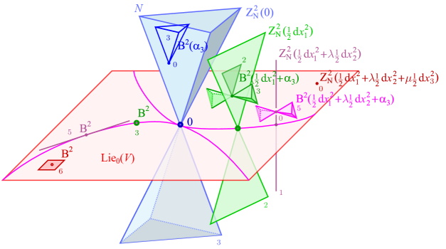
Figure 1: The Bianchi variety.

Figure 1 visualizes Lemma 5. The four “vertical” linear spaces, crossing the “horizontal” plane $\mathrm{Lie\,}_{0}(V)$, represent the $\zeta$–fibers attached to the rank–0 Lie structure (blue point), to a rank–1 structure (green point), to a rank–2 structure (purple poin), and to a non–degenerate structure (red point).

The disassembling property of Lie structures leads to a natural factorization of the action of $\mathrm{GL\,}(V)$ on $\mathrm{Lie\,}(V)$. Namely, $\mathrm{GL\,}(V)$ preserves $\zeta$. In view of that, the study of the moduli space $\frac{\mathrm{Lie\,}(V)}{\mathrm{GL\,}(V)}$ naturally splits into two steps. The first of them is to describe the moduli space of the symmetric bilinear forms (which is well–known for some fields $\mathbb{F}$), while the second is to describe the moduli space $\frac{Z^{2}_{N}(dF)}{\mathrm{Stab\,}(dF)}$.

To this end consider the subvariety $\Sigma\stackrel{{\scriptstyle\mathrm{def}}}{{=}}\{(dF,\psi)\ |\ \psi\in\mathrm{Stab\,}(dF)\}\subseteq\mathrm{Lie\,}_{0}(V)\times\mathrm{GL\,}(V)$ and its natural projection $\sigma:\Sigma\longmapsto\mathrm{Lie\,}_{0}(V)$, $(dF,\psi)\longmapsto dF$. Now fix an orbit $\Omega\stackrel{{\scriptstyle\mathrm{def}}}{{=}}\mathrm{GL\,}(V)\cdot dF$ of the $\mathrm{GL\,}(V)$–action on $\mathrm{Lie\,}_{0}(V)$ (see Remark 2). Lemma 5 tells precisely that $\zeta|_{\Omega}$ is a $(3-\mathrm{rank\,}dF)$–dimensional vector bundle over $\Omega$.

Observe that $\sigma|_{\Omega}$ is a principal group bundle over $\Omega$, acting on $\zeta|_{\Omega}$.

Lemma 6.

The quotient bundle $\frac{\zeta|_{\Omega}}{\sigma|_{\Omega}}$ is endowed with an absolute parallelism and, therefore, it is trivial.

Proof.

Take $dF,dG\in\Omega$, and choose $\varphi\in\mathrm{GL\,}(V)$ such that $dG=\varphi^{*}(dF)$. Define parallel displacement $t:\left(\frac{\zeta|_{\Omega}}{\sigma|_{\Omega}}\right)^{-1}(dF)\longrightarrow\left(\frac{\zeta|_{\Omega}}{\sigma|_{\Omega}}\right)^{-1}(dG)$,

$$t(\mathrm{Stab\,}(dF)\cdot(dF+\alpha))\stackrel{{\scriptstyle\mathrm{def}}}{{=}}\mathrm{Stab\,}(dG)\cdot(dG+\varphi^{*}(\alpha)),$$ (16)

and prove that (16) does not depend on the choice of $\alpha$ and $\varphi$.

If $\alpha^{\prime}$ is another choice of the non–unimodular charge of the orbit of $dF+\alpha$, then $\alpha^{\prime}=\phi^{*}(\alpha)$, with $\phi\in\mathrm{Stab\,}(dF)$. So, $\varphi^{-1}\phi\varphi\in\mathrm{Stab\,}(dG)$ implies that $\mathrm{Stab\,}(dG)\cdot(dG+\varphi^{*}(\alpha))=\mathrm{Stab\,}(dG)\cdot(dG+(\varphi^{-1}\phi\varphi)^{*}(\varphi^{*}(\alpha)))=\mathrm{Stab\,}(dG)\cdot(dG+\varphi^{*}(\phi^{*}(\alpha)))=\mathrm{Stab\,}(dG)\cdot(dG+\varphi^{*}(\alpha^{\prime}))$.

If $\overline{\varphi}$ is another transformation such that $dG=\overline{\varphi}^{*}(dF)$, then $\varphi^{-1}\overline{\varphi}\in\mathrm{Stab\,}(dG)$. Hence, $\mathrm{Stab\,}(dG)\cdot(dG+\varphi^{*}(\alpha))=\mathrm{Stab\,}(dG)\cdot(dG+(\varphi^{-1}\overline{\varphi})^{*}(\varphi^{*}(\alpha)))=\mathrm{Stab\,}(dG)\cdot(dG+\overline{\varphi}^{*}(\alpha))$. ∎

Let $c=c_{F}+c_{\alpha}$ be a Lie structure. The orbit $GL(V)\cdot\alpha_{c}$ of $\alpha_{c}$ is precisely the only parallel section of $\frac{\zeta|_{\Omega}}{\sigma|_{\Omega}}$ which takes the value $\mathrm{Stab\,}(dF)\cdot\alpha$ at the point $dF$. In other words, we have proved the main

Theorem 1.

The orbit space $\frac{\mathrm{Lie\,}(V)}{\mathrm{GL\,}(V)}$ is fibered over the orbit space $\frac{S^{2}(V)}{\mathrm{GL\,}(V)}$, the fiber at $\Omega$ being given by the set of parallel sections of $\frac{\zeta|_{\Omega}}{\sigma|_{\Omega}}$.

So, we have the following algorithm for describing orbits of Lie structures:

1. find the orbits of the action of $\mathrm{GL\,}(V)$ on $\mathrm{Lie\,}_{0}(V)$;

2. find the parallel sections of $\frac{\zeta|_{\Omega}}{\sigma|_{\Omega}}$, for any orbit $\Omega$ coming from the first step.

The evident advantage of this procedure is that the fibers of $\zeta$ and $\sigma$ are much smaller than $\mathrm{Lie\,}(V)$ and $\mathrm{GL\,}(V)$, respectively. Moreover, as we shall see, the second step does not depend on the field $\mathbb{F}$.

Remark 4.

Even in the case when the orbit space $\frac{S^{2}(V)}{\mathrm{GL\,}(V)}$ is not known, elements of $\mathrm{Lie\,}_{0}(V)$ are distinguished by their ranks (see [5]). Degenerate forms fill up a cubic hypersurface (purple curve in Fig. 1), which in its turn contains a closed subset of rank–one forms (green points in Fig. 1).

Let $c=c_{F}+c_{\alpha}$ be a Lie structure, and $\Omega$ the orbit of $dF$ in $\mathrm{Lie\,}_{0}(V)$.

Lemma 7.

$\zeta|_{\mathrm{GL\,}(V)\cdot\alpha_{c}}$ is a bundle over $\Omega$ with the fiber $\mathrm{Stab\,}(dF)\cdot\alpha$.

Proof.

Since $\mathrm{GL\,}(V)$ acts as a bundle automorphism on $\zeta|_{\mathrm{GL\,}(V)\cdot\alpha_{c}}$, it suffices to compute the fiber $\zeta|_{\mathrm{GL\,}(V)\cdot\alpha_{c}}^{-1}(dF)$. An element $c^{\prime}=c_{F}+c_{\alpha^{\prime}}$ is in such a fiber if and only if $dF+\alpha^{\prime}\in\mathrm{GL\,}(V)\cdot\alpha_{c}$, i.e., $\alpha^{\prime}=\psi^{*}(\alpha)$, with $\psi\in\mathrm{Stab\,}(dF)$. ∎

Corollary 2.

$\dim\mathrm{GL\,}(V)\cdot\alpha_{c}=\dim(\mathrm{GL\,}(V)\cdot dF)+\dim\mathrm{Stab\,}(dF)\cdot\alpha$.

This corollary suggests a formula for computing $\dim B^{2}(c)$,

$$\dim B^{2}(c)=\dim B^{2}(c_{F})+\dim\left(\frac{\mathrm{Stab\,}(dF)}{\mathrm{Stab\,}(dF)\cap\mathrm{Stab\,}(\alpha)}\right),$$

whose “infinitesimal version” is

$$\dim\left(\frac{\mathrm{End\,}(V)}{\mathrm{sym\,}(dF+\alpha)}\right)=\dim\left(\frac{\mathrm{End\,}(V)}{\mathrm{sym\,}(dF)}\right)+\dim\left(\frac{\mathrm{sym\,}(dF)}{\mathrm{sym\,}(dF)\cap\mathrm{sym\,}(\alpha)}\right).$$ (17)

Remark 5.

Notice that $\mathrm{sym\,}(dF+\alpha)=\mathrm{sym\,}(dF)\cap\mathrm{sym\,}(\alpha)$.

4 Computations

4.1 Unimodular structures

In the case $\alpha=0$ Lemma 7 says that the orbit of $\alpha_{c}$ coincides with $\Omega$. In view of (17), in order to find its dimension, it is sufficient to compute $\dim[\mathrm{sym\,}(dF)]$ (Proposition 5).

Proposition 5.

$$\dim B^{2}(dF)=\left\{\begin{array}[]{cc}6&\textrm{if }\mathrm{rank\,}dF=3\\ 5&\textrm{if }\mathrm{rank\,}dF=2\\ 3&\textrm{if }\mathrm{rank\,}dF=1\end{array}\right.$$

Proof.

We shall show that

$$\dim[\mathrm{sym\,}(dF)]=\left\{\begin{array}[]{cc}3&\textrm{ if }\mathrm{rank\,}dF=3\\ 4&\textrm{ if }\mathrm{rank\,}dF=2\\ 6&\textrm{ if }\mathrm{rank\,}dF=1.\end{array}\right.$$

To this end, prove that $\varphi\in\mathrm{sym\,}(\frac{1}{2}d(x_{1}^{2}+\lambda x_{2}^{2}+\mu x_{3}^{2}))$ if and only if

$$X_{\varphi}=(-\lambda ax_{2}-\mu bx_{3})\frac{\partial}{\partial x_{1}}+(ax_{1}+cx_{2}+ex_{3})\frac{\partial}{\partial x_{2}}+(bx_{1}+fx_{2}+dx_{3})\frac{\partial}{\partial x_{3}},$$ (18)

with the coefficients $a,\ldots,f$ satisfying conditions

$$\left\{\begin{array}[]{c}\lambda c=0\\ \mu d=0\\ \lambda e+\mu f=0.\end{array}\right.$$ (19)

Indeed, since $L_{X_{\varphi}}(\frac{1}{2}d(x_{k}^{2}))=(\varphi_{i}^{j}x_{j}\frac{\partial}{\partial x_{i}})(\frac{1}{2}d(x_{k}^{2}))=\frac{1}{2}d((\varphi_{i}^{j}x_{j}\frac{\partial}{\partial x_{i}})(x_{k}^{2}))=d(\varphi_{i}^{j}x_{j}\delta_{k}^{i}x_{k})=\varphi_{k}^{j}dx_{j}x_{k},$ the Lie derivative

$$L_{X_{\varphi}}({\textstyle\frac{1}{2}}d(x_{1}^{2}+\lambda x_{2}^{2}+\mu x_{3}^{2})) =\varphi_{1}^{1}{\textstyle\frac{1}{2}}d(x_{1}^{2})+\lambda\varphi_{2}^{2}{\textstyle\frac{1}{2}}d(x_{2}^{2})+\mu\varphi_{3}^{3}{\textstyle\frac{1}{2}}d(x_{3}^{2})$$

$$+(\varphi_{1}^{2}+\lambda\varphi_{2}^{1})d(x_{1}x_{2})+(\mu\varphi_{3}^{1}+\varphi_{1}^{3})d(x_{3}x_{1})+(\lambda\varphi_{2}^{3}+\mu\varphi_{3}^{2})d(x_{2}x_{3})$$

vanishes if and only if $X_{\varphi}$ can be put in the form (18), with coefficients satisfying (19). ∎

In the left side of Figure 1 the spaces $B^{2}(dF)$, whose dimension was computed in Proposition 5, are drawn as tangent spaces to $\mathrm{Lie\,}_{0}(V)$.

Proposition 6.

$\dim Z^{2}(c_{F})=9-\mathrm{rank\,}dF$.

Proof.

Observe that $Z^{2}(c_{F})=\mathrm{Lie\,}_{0}(V)\oplus Z_{N}^{2}(dF)$ and apply Lemma 5. ∎

Figure 1 makes evident Proposition 6. Indeed, $Z^{2}(c_{F})$ is precisely the space spanned by the “horizontal” subspace $\mathrm{Lie\,}_{0}(V)$ and the “vertical” subspaces $Z_{N}^{2}(dF)$.

The above results concerning the orbits of unimodular structures are summarized in the next table for $\mathbb{F}=\mathbb{R}$.

Type	Bianchi type(s)	Lie structure(s)	$\mathrm{rank\,}dF$	$\dim\mathrm{GL\,}(V)\cdot dF$	$\dim Z_{N}^{2}(dF)$	$\dim Z^{2}(c_{F})$	$\dim H^{2}(c_{F})$
$A_{0}$	AI	Abelian	0	0	3	9	9
$A_{1}$	AII	Heisenberg	1	3	2	8	5
$A_{2}^{-}$, $A_{2}^{+}$	AVI0, AVII0	$\mathfrak{e}(1,1)$, $\mathfrak{e}(2)$	2	5	1	7	2
$A_{3}^{-}$, $A_{3}^{+}$	AVIII, AIX	$\mathfrak{o}(2,1)$, $\mathfrak{o}(3)$	3	6	0	6	0

Remark 6.

In this table we introduce a new notation for isomorphism classes of three–dimensional Lie algebras, hoping it will be more informative. The original Bianchi notation can be found in [10].

4.2 Non–unimodular structures

4.2.1 $\mathrm{rank\,}dF=0$.

Then $dF=0$, $\Omega=\mathrm{GL\,}(V)\cdot dF=\{0\}$, $Z_{N}^{2}(0)=N$ and $\mathrm{Stab\,}(c_{F})=\mathrm{GL\,}(V)$. In other words, $\frac{\zeta|_{\Omega}}{\sigma|_{\Omega}}$ consists of just one fiber, which identifies with

$$\frac{N}{\mathrm{GL\,}(V)}.$$ (20)

Independently on the field $\mathbb{F}$, it can be easily proved (see [13]) the following

Proposition 7.

The moduli space (20) consists of two orbits, one of which is 0.

Proposition 8.

$\varphi\in\mathrm{sym\,}(\alpha_{3})$ if and only if

$$X_{\varphi}=(ax_{1}+bx_{2})\frac{\partial}{\partial x_{1}}+(cx_{1}-ax_{2})\frac{\partial}{\partial x_{2}}+(dx_{1}+ex_{2}+fx_{3})\frac{\partial}{\partial x_{3}}.$$ (21)

Proof.

It directly follows from

$$L_{X_{\varphi}}(\alpha_{3}) =(\varphi_{i}^{j}x_{j}{\textstyle\frac{\partial}{\partial x_{i}}})(x_{1}dx_{2}-x_{2}dx_{1})=$$

$$=\varphi_{i}^{j}x_{j}\delta_{1}^{i}dx_{2}+x_{1}d(\varphi_{i}^{j}x_{j}\delta_{2}^{i})-\varphi_{i}^{j}x_{j}\delta_{2}^{i}dx_{1}-x_{2}d(\varphi_{i}^{j}x_{j}\delta_{1}^{i})=$$

$$=\varphi_{1}^{j}(x_{j}dx_{2}-x_{2}dx_{j})+\varphi_{2}^{j}(x_{1}dx_{j}-x_{j}dx_{1})=-\varphi_{1}^{3}\alpha_{1}-\varphi_{2}^{3}\alpha_{2}+(\varphi_{1}^{1}+\varphi_{2}^{2})\alpha_{3}.$$

∎

The “vertical” blue subspace in Figure 1 is $N$. The 3–dimensional space $B^{2}(\alpha_{3})$ is shown inside $N$.

Notice that when $\mathbb{F}=\mathbb{R}$ or $\mathbb{C}$, Proposition 8 is sufficient to prove that the orbit of $\alpha_{3}$ is 3–dimensional and, therefore, it coincides with $N\smallsetminus\{0\}$.

4.2.2 $\mathrm{rank\,}dF=1$.

Independently on the field $\mathbb{F}$, all rank–1 elements of $\mathrm{Lie\,}_{0}(V)$ belong to the same orbit $\Omega=\mathrm{GL\,}(V)\cdot{\textstyle\frac{1}{2}}d(x_{1}^{2})$. To compute the fiber of $\frac{\mathrm{Lie\,}(V)}{\mathrm{GL\,}(V)}$ over $\Omega$, it suffices to compute the moduli space

$$\frac{Z_{N}^{2}({\textstyle\frac{1}{2}}d(x_{1}^{2}))}{\mathrm{Stab\,}({\textstyle\frac{1}{2}}d(x_{1}^{2}))}$$ (22)

(see Theorem 1).

Observe that $Z_{N}^{2}({\textstyle\frac{1}{2}}d(x_{1}^{2}))$ is the 2–dimensional vector space spanned by $\alpha_{2}$ and $\alpha_{3}$ (see the proof of Lemma 5). Fix a non–zero element $a\alpha_{2}+b\alpha_{3}$. Then it is possible to choose an automorphism $\psi\in\mathrm{GL\,}(V)$ which preserves $x_{1}$ and sends $bx_{2}-ax_{3}$ to $x_{2}$. In other words, $\psi\in\mathrm{Stab\,}({\textstyle\frac{1}{2}}d(x_{1}^{2}))$ and $\psi^{*}(a\alpha_{2}+b\alpha_{3})=\alpha_{3}$, thus proving the following

Proposition 9.

The moduli space (22) consists of two orbits, one of which is 0.

4.2.3 $\mathrm{rank\,}dF=2$.

The orbits of rank–2 structures in $\mathrm{Lie\,}_{0}(V)$ are $\Omega=\mathrm{GL\,}(V)\cdot dF$, $F={\textstyle\frac{1}{2}}(x_{1}^{2}+\epsilon x_{2}^{2})$, with $\epsilon\in\mathbb{F}$ (see [5]). Recall that $Z_{N}^{2}(dF)$ is the 1–dimensional subspace spanned by $\alpha_{3}$ (see the proof of Lemma 5).

We shall show that the fiber over $\Omega$ is $\mathbb{F}$.

Proposition 10.

Let $\mathbb{F}$ be $\mathbb{R}$ (resp., $\mathbb{C}$). Then the moduli space

$$\frac{Z_{N}^{2}(dF)}{(\mathrm{Stab\,}dF)},\quad F={\textstyle\frac{1}{2}}(x_{1}^{2}+\epsilon x_{2}^{2}),\epsilon=\pm 1\ (\textrm{resp.}\ 1)$$ (23)

coincides with $\langle\alpha_{3}\rangle$.

Proof.

Notice that he stabilizer in $\mathrm{Stab\,}(dF)$ of an element $\lambda\alpha_{3}\in Z_{N}^{2}(dF)$ coincides with $\mathrm{Stab\,}(\lambda\alpha_{3})\cap\mathrm{Stab\,}(dF)$. To prove the result, it suffices to show that $\mathrm{Stab\,}(dF)$ is contained in $\mathrm{Stab\,}(\lambda\alpha_{3})$.

This is obvious for $\lambda=0$. For $\lambda\neq 0$ we, first, observe that $\mathrm{Stab\,}(\lambda\alpha_{3})=\mathrm{Stab\,}(\alpha_{3})$. Then, it follows from Propositions 5 and 8 that a symmetry of $dF$ is also a symmetry of $\alpha_{3}$. ∎

The proof of the above proposition is simplified by infinitesimal arguments, which does not work if $\mathbb{F}$ is different from $\mathbb{R}$ or $\mathbb{C}$. For a generic $\mathbb{F}$ see [13].

4.2.4 Cocycles of non–unimodular Lie structures

Lemma 8.

If $c$ is a non–unimodular Lie structures, then $\dim Z^{2}(c)=6$.

Proof.

Any non–unimodular Lie structure is equivalent to $c_{{\textstyle\frac{1}{2}}(\lambda x_{1}^{2}+\mu x_{2}^{2})}+c_{\alpha_{3}}$. Let $dF=d({\textstyle\frac{1}{2}}(ax_{1}^{2}+bx_{2}^{2}+cx_{3}^{2})+ex_{2}x_{3}+fx_{1}x_{3}+gx_{1}x_{2})$ (resp., $\alpha=k\alpha_{1}+l\alpha_{2}+m\alpha_{3}$) be an arbitrary element of $\mathrm{Lie\,}_{0}(V)$ (resp., $N$). Then, independently on $\lambda$ and $\mu$, the commutator

$$[[c_{{\textstyle\frac{1}{2}}(\lambda x_{1}^{2}+\mu x_{2}^{2})}+c_{\alpha_{3}},c_{F}+c_{\alpha}]] =[[c_{{\textstyle\frac{1}{2}}(\lambda x_{1}^{2}+\mu x_{2}^{2})},c_{\alpha}]]$$

$$+[[c_{{\textstyle\frac{1}{2}}(ax_{1}^{2}+bx_{2}^{2}+cx_{3}^{2})+ex_{2}x_{3}+fx_{1}x_{3}+gx_{1}x_{2}},c_{\alpha_{3}}]]$$

$$=(k\lambda 2x_{1}+l\mu 2x_{2}+c2x_{3}+2ex_{2}+2fx_{1})\boldsymbol{\xi}$$

$$=2((f+k\lambda)x_{1}+(e+l\mu)x_{2}+cx_{3})\boldsymbol{\xi}$$

vanishes if and only if the three equations $f+k\lambda=0$, $e+l\mu=0$ and $c=0$ are satisfied. ∎

The obtained results are summarized in the following table, where $c=c_{F}+c_{\alpha}$.

Type	Bianchi type(s)	$\mathrm{rank\,}dF$	$\dim B^{2}(c)$	$\dim Z^{2}(c)$	$\dim H^{2}(c)$
$B_{0}$	V	0	3	6	3
$B_{1}$	IV	1	5	6	1
$B_{2,\lambda}^{\pm}$	III, VIh, VIIh	2	5	6	1

5 Compatibility varieties

Let $c\in\mathrm{Lie\,}(V)$.

Definition 2.

The affine algebraic variety $\mathrm{Lie\,}(V,c)\stackrel{{\scriptstyle\mathrm{def}}}{{=}}\mathrm{Lie\,}(V)\cap Z^{2}(c)\subseteq Z^{2}(c)$ is called the compatibility variety of $c$.

Obviously, $\mathrm{Lie\,}(V,c)$ can be understood as the set of Lie structures which are compatible with $c$, or as the union of all linear subspace of $\mathrm{Lie\,}(V)$ passing through $c$. So, $\mathrm{Lie\,}(V,c)$ is a conic variety.

The canonical disassembling of $\mathrm{Lie\,}(V)$ and other results of Section 3 are reproduced as well for the compatibility variety $\mathrm{Lie\,}(V,c)$, with unimodular $c$. In particular, $\mathrm{Lie\,}_{0}(V)\subseteq\mathrm{Lie\,}(V,c_{F})$ for any $F$. Consider the map $\zeta^{F}\stackrel{{\scriptstyle\mathrm{def}}}{{=}}\pi_{0}|_{\mathrm{Lie\,}(V,c_{F})}$. Then we have

$$(\zeta^{F})^{-1}(dG)=Z_{N}^{2}(dG)\cap Z_{N}^{2}(dF).$$

5.1 Computations

In this subsection we shall describe the varieties $\mathrm{Lie\,}(V,c)$, for all types of structures $c$. Obviously, $\mathrm{Lie\,}(V,0)=\mathrm{Lie\,}(V)$, so we assume $c\neq 0$.

We introduce the notation

$$s^{2}\stackrel{{\scriptstyle\mathrm{def}}}{{=}}\mathrm{span\,}\{{\textstyle\frac{1}{2}}d(x_{1}^{2}),{\textstyle\frac{1}{2}}d(x_{2}^{2}),{\textstyle\frac{1}{2}}d(x_{1}x_{2})\}.$$

Notice that $s^{2}$ identifies with the space of symmetric bilinear forms on $\mathrm{span\,}\{\xi^{1},\xi^{2}\}$.

5.1.1 Compatibility variety of $A_{3}^{\pm}$ structures

Let $c=c_{F}$. If $\mathrm{rank\,}(F)=3$, then $Z_{N}^{2}(dF)=0$ and $\mathrm{Lie\,}(V,c)=\mathrm{Lie\,}_{0}(V)$ is a 6–dimensional vector subspace (see Fig. 2).

Figure 2: Only when $c$ is an unimodular structure of type $A_{3}^{\pm}$, $\mathrm{Lie\,}(V,c)$ is a linear space.

5.1.2 Compatibility variety of $A_{2}^{\pm}$ structures

Let now $F={\frac{1}{2}}(x_{1}^{2}+\epsilon x_{2}^{2})$, $\epsilon\in\mathbb{F}\smallsetminus\{0\}$.

Lemma 9.

$Z^{2}(\alpha_{3})\cap\mathrm{Lie\,}_{0}(V)=s^{2}$.

Proof.

Immediately from Proposition 4. ∎

Proposition 11.

$\mathrm{Lie\,}(V,c_{F})$ is the union

$$\mathrm{Lie\,}(V,c_{F})=\mathrm{Lie\,}_{0}(V)\cup\mathrm{span\,}\{s^{2},\alpha_{3}\}$$ (24)

of a 6–dimensional and a 4–dimensional subspace, intersecting along the 3–dimensional subspace $s^{2}$.

Proof.

Obviously, the right–hand side of (24) is contained in the left one. Let $c^{\prime}=c_{G}+\alpha\in\mathrm{Lie\,}(V,c_{F})$ with $\alpha\neq 0$.

Since $c^{\prime}$ is compatible with $c_{F}$, $dF\wedge d\alpha_{c^{\prime}}=0$. But $dF\wedge d\alpha_{c^{\prime}}=dF\wedge d\alpha$, so $dF\wedge d\alpha=0$, i.e. $\alpha\in Z_{N}^{2}(dF)$. In view of Lemma 5, $Z_{N}^{2}(dF)$ is the one–dimensional subspace generated by $\alpha_{3}$. Hence $\alpha=\lambda\alpha_{3}$, $\lambda\neq 0$.

This shows that $c_{G}$, being compatible with $\alpha$, is compatible with $\alpha_{3}$ and, by Lemma 9, is a linear combination of $\frac{1}{2}d(x_{1}^{2}),\frac{1}{2}d(x_{2}^{2}),d(x_{1}x_{2})$. ∎

Figure 3 shows that the structure of $\mathrm{Lie\,}(V,c_{F})$ is quite simple. The 3–dimensional subspace $s^{2}$ is precisely the locus where the fibers of $\zeta^{F}$ are nontrivial. The restriction of $\zeta^{F}$ to it is a trivial bundle with fiber $\mathrm{span\,}\{\alpha_{3}\}$.

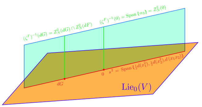
Figure 3: The compatibility variety af a structure $c_{F}$ of type $A_{2}^{\pm}$.

5.1.3 Compatibility variety of $A_{1}$ structures

This case is more complicated (see Fig. 4). Let $F={\textstyle\frac{1}{2}}x_{1}^{2}$.

Proposition 12.

If $(0,0)\neq(a,b)\in\mathbb{F}^{2}$, then $\zeta^{F}$ is a rank–2 trivial bundle over the line $\mathrm{span\,}\{{\textstyle\frac{1}{2}}d(x_{1}^{2})\}$ with the fiber $\mathrm{span\,}\{\alpha_{2},\alpha_{3}\}$, and over $\mathrm{span\,}\{{\textstyle\frac{1}{2}}d(x_{1}^{2}),{\textstyle\frac{1}{2}}d((bx_{2}-ax_{3})^{2})\}\smallsetminus\mathrm{span\,}\{{\textstyle\frac{1}{2}}d(x_{1}^{2})\}$, $\zeta^{F}$ is a rank–1 trivial bundle with the fiber $\mathrm{span\,}\{a\alpha_{2}+b\alpha_{3}\}$. Fibers of $\zeta^{F}$ are trivial over the rest of $\mathrm{Lie\,}_{0}(V)$.

Proof.

As it follows from Lemma 5, $Z_{N}^{2}(dF)=\mathrm{span\,}\{\alpha_{2},\alpha_{3}\}$. Therefore, the intersection $Z_{N}^{2}(dF)\cap Z_{N}^{2}(dG)$ is 2–dimensional if and only if $Z_{N}^{2}(dF)=Z_{N}^{2}(dG)$, i.e., if $dG$ belongs to the line $\mathrm{span\,}\{{\textstyle\frac{1}{2}}d(x_{1}^{2})\}$.

The intersection $Z_{N}^{2}(dF)\cap Z_{N}^{2}(dG)$ can be of dimension 1 in the following two cases. First, $Z_{N}^{2}(dG)$ is a 2–dimensional subspace intersecting $\mathrm{span\,}\{\alpha_{2},\alpha_{3}\}$ along a line, and, second, $Z_{N}^{2}(dG)$ is a 1–dimensional subspace contained in $\mathrm{span\,}\{\alpha_{2},\alpha_{3}\}$.

In the first case, a line in $\mathrm{span\,}\{\alpha_{2},\alpha_{3}\}$ can be written as $\mathrm{span\,}\{a\alpha_{2}+b\alpha_{3}\}$, with $(0,0)\neq(a,b)$. Then $dG={\textstyle\frac{1}{2}}d((bx_{2}-ax_{3})^{2})$ is the only rank–1 structure such that $Z_{N}^{2}(dG)$ intersects $\mathrm{span\,}\{\alpha_{2},\alpha_{3}\}$ along $\mathrm{span\,}\{a\alpha_{2}+b\alpha_{3}\}$.

In the second case, $dG$ must be a rank–2 structure such that $Z_{N}^{2}(dG)$ is precisely $\mathrm{span\,}\{a\alpha_{2}+b\alpha_{3}\}$. Up to proportionality, this is $G={\textstyle\frac{1}{2}}(x_{1}^{2}+(bx_{2}-ax_{3})^{2})$. ∎

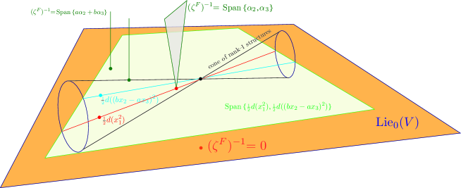
Figure 4: The compatibility variety af a structure $c_{F}$ of type $A_{1}$.

5.1.4 Compatibility varieties of $B_{0}$ structures

If $\alpha_{i}$ (resp., $d(x_{i}x_{j})$) is a base vector of $N$ (resp., $\mathrm{Lie\,}_{0}(V)$), then the dual to it covector will denoted by $\alpha_{i}^{\circ}$ (resp., $d(x_{i}x_{j})^{\circ}$).

As it follows from Lemma 8, the space of 2–cocycles of the structure $c_{F}+c_{\alpha_{3}}$, with $F={{\textstyle\frac{1}{2}}(\lambda x_{1}^{2}+\mu x_{2}^{2})}$, is the 6–dimensional space

$$\mathrm{span\,}\{s^{2},\alpha_{1}-\lambda d(x_{1}x_{3}),\alpha_{2}-\mu d(x_{2}x_{3}),\alpha_{3}\}.$$ (25)

If $c$ is a structure of type $B_{0}$, i.e., $\lambda=\mu=0$, then

$$\mathrm{Lie\,}(V,c)=\zeta^{-1}(s^{2}).$$ (26)

$\zeta|_{\mathrm{Lie\,}(V,c)}$ is a stratified vector bundle over $s^{2}$. Indeed (see Lemma 5), $\zeta$ is of rank 3 over $\{0\}$, it is of rank 2 over the quadric $d(x_{1}^{2})^{\circ}d(x_{2}^{2})^{\circ}-(d(x_{1}x_{2})^{\circ})^{2}=0$, and it is of rank 1 over the rest of $s^{2}$ (see Fig. 5).

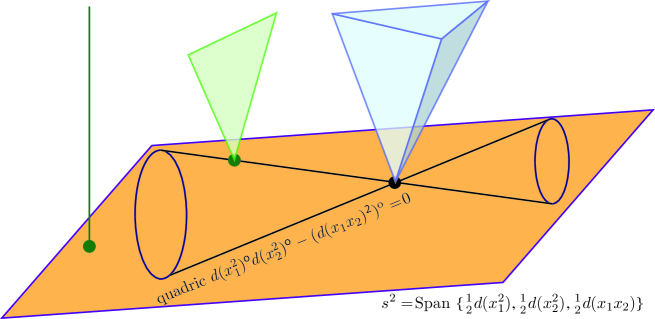
Figure 5: The compatibility variety of a non–unimodular Lie structure of type $B_{0}$.

5.1.5 Compatibility varieties of $B_{1}$ structures

If $c$ is a structure of type $B_{1}$, then $\lambda=1$ and $\mu=0$. Directly from (25) it follows that $\mathrm{Lie\,}(V,c)$ is the intersection of $\zeta^{-1}(\mathrm{span\,}\{s^{2},d(x_{1}x_{3})\})$ with the affine hyperplane $(\alpha_{1})^{\circ}=-(d(x_{1}x_{3}))^{\circ}$. Moreover, if $c_{G}+ad(x_{1}x_{3})+\alpha\in\mathrm{Lie\,}(V,c)$, with $c_{G}\in s^{2}$, it is easy to prove that $a=0$. In other words,

$$\mathrm{Lie\,}(V,c)=\zeta^{-1}(s^{2})\cap\{(\alpha_{1})^{\circ}=0\},$$ (27)

i.e., $\zeta|_{\mathrm{Lie\,}(V,c)}$ is a stratified vector bundle over $s^{2}$, whose fibers are subspaces of the corresponding fibers of $\zeta$.

Describe now the corresponding strata. Let $c_{G}+\alpha\in\mathrm{Lie\,}(V,c)$. If $c_{G}\in\mathrm{span\,}\{{\textstyle\frac{1}{2}}d(x_{1}^{2})\}$ then $\zeta|_{\mathrm{Lie\,}(V,c)}^{-1}(c_{G})=\mathrm{span\,}\{\alpha_{2},\alpha_{3}\}$. If $c_{G}$ is a point of the quadric $d(x_{1}^{2})^{\circ}d(x_{2}^{2})^{\circ}-(d(x_{1}x_{2})^{\circ})^{2}=0$, not belonging to the line $\mathrm{span\,}\{{\textstyle\frac{1}{2}}d(x_{1}^{2})\}$, then $\zeta|_{\mathrm{Lie\,}(V,c)}^{-1}(c_{G})$ is the 1–dimensional subspace $(\alpha_{1})^{\circ}=0$ of $\zeta^{-1}(c_{G})$. If $c_{G}$ is not in the quadric above, then $\zeta|_{\mathrm{Lie\,}(V,c)}^{-1}(c_{G})$ coincides with $\zeta^{-1}(c_{G})$, i.e., $\mathrm{span\,}\{\alpha_{3}\}$ (see Fig. 6).

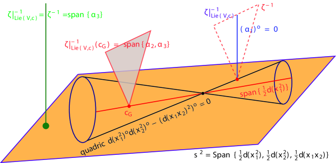
Figure 6: The compatibility variety of a non–unimodular Lie structure of type $B_{1}$.

5.1.6 Compatibility varieties of $B_{2,\nu}^{\pm}$ structures

Finally, if $\lambda=\pm\mu=\nu^{-1}$, then $c$ is a structure of type $B_{2,\nu}^{\pm}$. In this case $\mathrm{Lie\,}(V,c)$ is the intersection of $\zeta^{-1}(\mathrm{span\,}\{s^{2},d(x_{1}x_{3}),d(x_{2}x_{3})\})$ with the affine subspace

$$\left\{\begin{array}[]{l}(\alpha_{1})^{\circ}=-\nu(d(x_{1}x_{3}))^{\circ}\\ (\alpha_{2})^{\circ}=\mp\nu(d(x_{2}x_{3}))^{\circ}.\end{array}\right.$$

Moreover, if $c^{\prime}=c_{G}+ed(x_{1}x_{3})+fd(x_{2}x_{3})+\alpha\in\mathrm{Lie\,}(V,c)$, with $c_{G}\in s^{2}$, it is easy to prove that $e^{2}=\pm f^{2}$.

If $e=f=0$, i.e., the unimodular component of $c^{\prime}$ belongs to $s^{2}$, then

$$\mathrm{Lie\,}(V,c)\cap\zeta^{-1}(s^{2})=\zeta^{-1}(s^{2})\cap\{(\alpha_{1})^{\circ}=(\alpha_{2})^{\circ}=0\},$$ (28)

i.e., the restriction of $\zeta|_{\mathrm{Lie\,}(V,c)}$ over $s^{2}$ is a trivial vector bundle with the fiber $\mathrm{span\,}\{\alpha_{3}\}$.

If $ef\neq 0$, then it is easy to prove that $c^{\prime}=ac+e(d(x_{1}x_{3})-\nu\alpha_{1})+f(d(x_{2}x_{3})\mp\nu\alpha_{2})$. In other words, the restriction of $\zeta|_{\mathrm{Lie\,}(V,c)}$ over the degenerate quadric $\{(d(x_{1}x_{3})^{\circ})^{2}\mp(d(x_{2}x_{3})^{\circ})^{2}=0\}\subseteq\mathrm{span\,}\{{\scriptstyle\frac{1}{2}}d(x_{1}^{2})\pm{\scriptstyle\frac{1}{2}}d(x_{2}^{2}),d(x_{1}x_{3}),d(x_{2}x_{3})\}$ is the graph of the map

$$a({\scriptstyle\frac{1}{2}}d(x_{1}^{2})\pm{\scriptstyle\frac{1}{2}}d(x_{2}^{2}))+ed(x_{1}x_{3})+fd(x_{2}x_{3})\longmapsto\nu(a\alpha_{3}-e\alpha_{1}\mp f\alpha_{2}).$$ (29)

Comparing (26), (27), (28) and (29), one observes that when the rank of the unimodular component of $c$ increases, the dimension of the fibers of $\zeta|_{\mathrm{Lie\,}(V,c)}$ over $s^{2}$ decreases. Observe that in all cases, $\mathrm{Lie\,}(V,c)\cap\mathrm{Lie\,}_{0}(V)=s^{2}$. It is worth also stressing that elements $c^{\prime}\in\mathrm{Lie\,}(V,c)$ such that $\zeta(c^{\prime})\not\in s^{2}$ exists only for structures $c$ of the type $B_{2,\nu}^{\pm}$ (see Fig. 7).

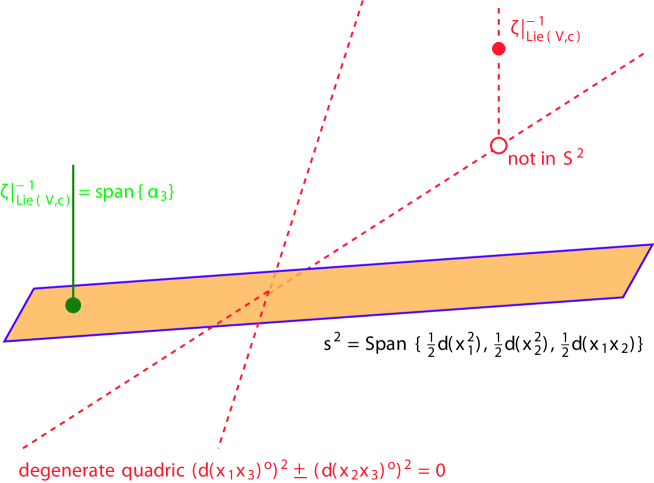
Figure 7: The compatibility variety of a non–unimodular Lie structure of type $B_{2,\nu}^{\pm}$.

5.2 Deformations of Lie structures

Recall that a (algebraic, smooth, continuous) deformation of a Lie structure $c$ is a (algebraic, smooth, continuous) curve in $\mathrm{Lie\,}(V)$, i.e., a map $\gamma:\mathbb{F}\longmapsto\mathrm{Lie\,}(V)$, passing through $c$.

Denote by $\mathcal{F}$ the algebra of algebraic functions on $\mathrm{Lie\,}(V)$, i.e., the quotient of $S(V\otimes_{\mathbb{F}}V)$ by the ideal generated by (2). If $\mathbb{F}=\mathbb{R}$, define also $C^{\infty}(\mathrm{Lie\,}(V))$ as the quotient of the algebra $C^{\infty}(V\otimes_{\mathbb{F}}V)$ by the ideal generated by (2). A map from $\mathbb{F}$ to $\mathrm{Lie\,}(V)$ is called alebraic (resp., smooth) if it corresponds to an algebra homomorphism $\mathcal{F}\longmapsto\mathbb{F}[x]$ (resp., $C^{\infty}(\mathrm{Lie\,}(V))\longmapsto C^{\infty}(\mathbb{R})$) in the sense of [1]. In particular, a linear map from $\mathbb{F}$ to $\mathrm{Lie\,}(V)$, i.e., an $\mathbb{F}$–homomorphsim from $\mathbb{F}$ to $V\otimes_{\mathbb{F}}V$ whose image is contained in $\mathrm{Lie\,}(V)$, is algebraic (and smooth, if $\mathbb{F}=\mathbb{R}$).

A defomation is called linear if $\gamma$ is a straight line. Observe that the linear deformation

$$\gamma_{d}(t)\stackrel{{\scriptstyle\mathrm{def}}}{{=}}(1-t)c+td$$ (30)

of $c$ is naturally associated with the element $d\in\mathrm{Lie\,}(V,c)$, $d\neq 0$. Obviously, any linear deformation of $c\in\mathrm{Lie\,}(V)$ is of the form $\gamma_{d}$.

We define an infinitesimal deformation to be tangent vector at $c$ of a deformation $\gamma$. In particular, the infinitesimal deformation associated with $\gamma_{d}$ is the affine vector $\gamma^{\prime}_{d}(0)$, connecting $c$ and $d$. Infinitesimal deformations must be understood as elements of the tangent space to $\mathrm{Lie\,}(V)$. Two infinitesimal deformations are called equivalent if one is obtained from another by action of $d_{c}\psi$, with $\psi\in\mathrm{Stab\,}(c)$.

The tangent space to $\mathrm{Lie\,}(V)$ is naturally identified with $Z^{2}(c)$, and the above described action of $\mathrm{Stab\,}(c)$ coincides with a natural action of $\mathrm{Stab\,}(c)$ on $Z^{2}(c)$. Moreover, the subset of $Z^{2}(c)$ that corresponds to the linear deformations coincides with $\mathrm{Lie\,}(V,c)$, and the action of $\mathrm{Stab\,}(c)$ restricts to it.

5.3 Some examples of deformations

Now we shall exploit the above description of $\mathrm{Lie\,}(V,c)$ in order to describe deformations of a 3–dimensional Lie structure $c$ and their equivalence classes as well. By abusing the language we shall call the quotient $\frac{\mathrm{Lie\,}(V,c)}{\mathrm{Stab\,}(c)}$ “orbit space”.

To this end, it will be necessary to consider some special subgroups of $\mathrm{GL\,}(V)$.

Remark 7.

If $F={\frac{1}{2}}(x_{1}^{2}+x_{2}^{2}\pm x_{3}^{2})$, then $\mathrm{Stab\,}(c_{F})$ is $O(3)$ (resp., $O(2,1)$) (see also Proposition 5). Similarly, for $F={\frac{1}{2}}(x_{1}^{2}\pm x_{2}^{2})$, the group $\mathrm{Stab\,}(c_{F})$ will be denoted $O(2,0)$ or $O(1,1,0)$, respectively. Finally, notice that $\mathrm{Stab\,}(c_{F})$, for $F={\frac{1}{2}}x_{1}^{2}$, coincides with the stabilizer of $x_{1}$. We do not describe the orbits of the action of $\mathrm{Stab\,}(c_{F})$ on $\mathrm{Lie\,}_{0}(V)$, since this concerns the theory of symmetric bilinear forms (see [5]).

Denote by $p:\mathrm{Lie\,}(V)\longmapsto\frac{\mathrm{Lie\,}(V)}{\mathrm{GL\,}(V)}$ a natural projection of sets. Recall that a (algebraic, smooth) deformation $\gamma$ of $c=\gamma(0)$ is called a contraction of $c$ if $p\circ\gamma$ takes two different values for $t=0$ and $t\neq 0$.

5.3.1 Deformations of $A_{3}^{+}$ structures

Let $F={\frac{1}{2}}(x_{1}^{2}+x_{2}^{2}+x_{3}^{2})$ and $c=c_{F}$. Then $\mathrm{Lie\,}(V,c)=\mathrm{Lie\,}_{0}(V)$ (see Subsection 5.1.1), and $\mathrm{Stab\,}(c)=O(3)$ (see Remark 7). Hence the orbit space identifies with $\frac{S^{2}(V)}{O(3)}$, i.e., with the space of diagonal 3 by 3 matrices over $\mathbb{F}$.

Observe that no deformation of $c$ is a contraction. The reader should not confuse between deformations of Lie algebras and deformations of Lie algebra structures.

5.3.2 Deformations of $A_{2}^{+}$ structures

Let $F={\frac{1}{2}}(x_{1}^{2}+x_{2}^{2})$ and $c=c_{F}$.

Observe that in this case $s^{2}$ is $O(2,0)$–invariant and the orbits of the restricted action of $O(2,0)$ are the same as the orbits of the natural action of $O(2)$ on $s^{2}$. It is easy to prove that the set of parallel sections of $\zeta^{F}|_{\Omega}$, for such an $\Omega$, is identified with $\mathbb{F}$.

Remark 8.

If intersection of two subspaces of a vector space is non–trivial, then there are smooth curves passing from one subspace to the other, in contrast with the algebraic ones. In particular there are smooth curves connecting any point of $\mathrm{Lie\,}_{0}(V)$ with any point of $\mathrm{span\,}\{s^{2},\alpha_{3}\}$ (See Figure 3). This is obviously not the case for algebraic curves. So, this example illustrates the difference between algebraic and smooth deformations.

5.3.3 Deformations of $A_{1}$ structures

Let $F={\frac{1}{2}}(x_{1}^{2})$ and $c=c_{F}$.

In this case, the line $\mathrm{span\,}\{\frac{1}{2}(x_{1}^{2})\}$ is $\mathrm{Stab\,}(c)$–invariant and the restricted action is trivial, i.e., $\Omega$ is a point. Similarly to Proposition 9, one proves that there is only one nonzero parallel section of $\zeta^{F}|_{\Omega}$.

Under the action of $\mathrm{Stab\,}(c)$, the plane $\mathrm{span\,}\{\frac{1}{2}(x_{1}^{2}),\frac{1}{2}((bx_{2}-ax_{3})^{2})\}$ (see Fig. 4) rotates around the axis $\mathrm{span\,}\{\frac{1}{2}(x_{1}^{2})\}$. If $\Omega$ is an orbit of $\mathrm{Stab\,}(c)$ not contained in this axis, then the set of parallel sections of $\zeta^{F}|_{\Omega}$ is identified with $\mathbb{F}$.

5.4 Effect of deformations on symplectic foliation in the case $\mathbb{F}=\mathbb{R}$

A deformation of a Lie structure $c$ induces a deformation of the symplectic foliation of $P^{c}$. Note that only the solvable 3–dimensional Lie stuctures admit non–trivial deformations. In such a case, $P^{c}$ can be brought to the form

$$P_{c}=X_{\phi}\wedge\frac{\partial}{\partial x^{3}},$$ (31)

with $\phi\in\mathrm{End\,}(\mathbb{R}^{2})$. Indeed, solvable Lie structures $B_{0}$, $B_{1}$, $B_{2,\lambda}^{\pm}$, and $A_{2}^{\pm}$ are of this form, with $\varphi$ being

$$\scriptsize{\left(\begin{array}[]{cc}-1&0\\ 0&-1\end{array}\right)},\ \scriptsize{\left(\begin{array}[]{cc}-1&1\\ 0&-1\end{array}\right)},\ \scriptsize{\left(\begin{array}[]{cc}-\lambda&1\\ \mp 1&-\lambda\end{array}\right)},\textrm{{\normalsize\ and }}\scriptsize{\left(\begin{array}[]{cc}0&1\\ \mp 1&0\end{array}\right)},$$

respectively. The nil-potent Lie structure $A_{1}$ corresponds to $\varphi=\scriptsize{\left(\begin{array}[]{cc}0&1\\ 0&0\end{array}\right)}$.

If $X_{\phi}=\phi_{a}^{b}x_{b}\frac{\partial}{\partial x_{a}}$, $a,b=1,2$, then $P^{c}=\phi_{a}^{b}x_{b}\frac{\partial}{\partial x_{a}}\wedge\frac{\partial}{\partial x_{3}}$,

$$\alpha_{c}=\frac{1}{2}\left(\phi_{2}^{1}dx_{1}^{2}-\phi_{1}^{2}dx_{2}^{2}\right)+\phi_{2}^{2}x_{2}dx_{1}-\phi_{1}^{1}x_{1}dx_{2},$$ (32)

and, therefore,

$$P^{c}_{x_{1}} = -\phi(x_{1})\frac{\partial}{\partial x^{3}},$$

$$P^{c}_{x_{2}} = -\phi(x_{2})\frac{\partial}{\partial x^{3}},$$

$$P^{c}_{x_{3}} = X_{\phi}.$$

Notice that in each point $p=(x_{1},x_{2},x_{3})$ where $\phi(x_{1})$ and $\phi(x_{2})$ are not simultaneously zero, $\mathrm{span\,}\{P^{c}_{x_{1}},P^{c}_{x_{2}}\}$ is the line generated by ${\scriptstyle\left.\frac{\partial}{\partial x^{3}}\right|_{p}}$. So, it holds the following lemma.

Lemma 10.

Symplectic leaves of a solvable Lie structure corresponding to Poisson bi–vector (31) are either pull–backs of trajectories of $X_{\phi}$ in $\mathbb{R}^{2}\smallsetminus\ker\phi$ via the projection $\mathbb{R}^{3}\longmapsto\mathbb{R}^{2}$, or single points of the subspace $\ker\phi\oplus\langle x_{3}\rangle$.

5.4.1 Deformation of $B_{2,\lambda}^{\pm}$ to $A_{2}^{\pm}$

In this case, elliptic (resp. hyperbolic) spirals converge to circles (resp. hyperbola), as $\lambda\to 0$. Since the $B_{2}^{\lambda}$’s are mutually non–isomorphic for different values of $\lambda$, such deformation is not a contraction.

5.4.2 Deformation of $B_{2,1}^{\pm}$ to $A_{1}$

Consider the family of structures $\{c_{\mu}^{\pm}\}_{\mu\in\mathbb{R}^{+}}$ of the form (31), with

$$\varphi_{\mu}^{\pm}={\left(\begin{array}[]{cc}-1&1\\ \mp\mu&-1\end{array}\right)}$$

and

$$\alpha_{c_{\mu}^{\pm}}=\frac{1}{2}(dx_{1}^{2}\pm\mu dx_{2}^{2})+\alpha_{3}.$$

Then the trajectory of $X_{\varphi_{\mu}^{\pm}}$ issuing from $(x_{1}^{0},x_{2}^{0})$, $x_{1}^{0}\neq 0$, is given by

$$x_{1}(t) = e^{-t}\sqrt{(x_{1}^{0})^{2}+\mu(x_{2}^{0})^{2}}\cos\left(\arctan\left(\sqrt{\mu}\frac{x_{2}^{0}}{x_{1}^{0}}\right)+\sqrt{\mu}t\right)$$

$$x_{2}(t) = e^{-t}\sqrt{\frac{(x_{1}^{0})^{2}}{\mu}+(x_{2}^{0})^{2}}\sin\left(\arctan\left(\sqrt{\mu}\frac{x_{2}^{0}}{x_{1}^{0}}\right)+\sqrt{\mu}t\right)$$

and

$$x_{1}(t) = \frac{x_{1}^{0}+\sqrt{\mu}x_{2}^{0}}{2}e^{(\sqrt{\mu}-1)t}+\frac{x_{1}^{0}-\sqrt{\mu}x_{2}^{0}}{2}e^{-(\sqrt{\mu}+1)t}$$

$$x_{2}(t) = \frac{x_{1}^{0}+\sqrt{\mu}x_{2}^{0}}{2\sqrt{\mu}}e^{(\sqrt{\mu}-1)t}-\frac{x_{1}^{0}-\sqrt{\mu}x_{2}^{0}}{2\sqrt{\mu}}e^{-(\sqrt{\mu}+1)t}$$

Trajectories of $X_{\varphi_{\mu}^{+}}$ (red) and of $X_{\varphi_{\mu}^{-}}$ (blue), issuing from vertices of a regular hexagon centered at the origin, are represented in Figure 8, for $\mu$ running from almost zero (first picture) to 1 (last picture). We see that both elliptic (determined by $c_{\mu}^{+}$) and hyperbolic (determined by $c_{\mu}^{-}$) spirals converge to the same foliation as $\mu\to 0$, and the constructed deformation is a contraction.

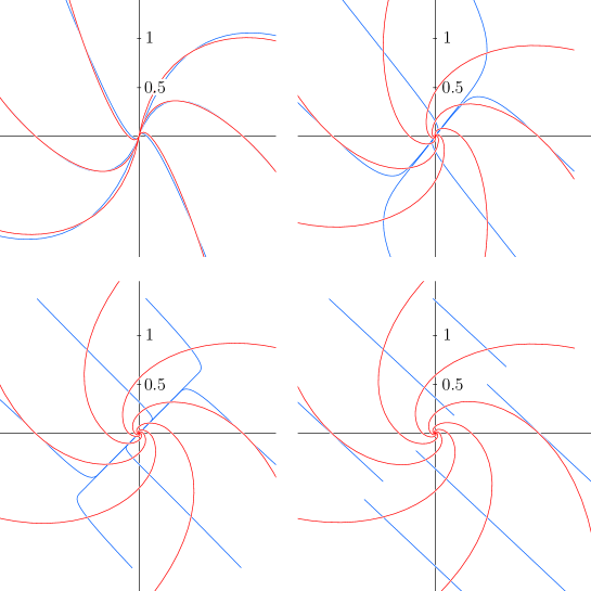
Figure 8: Projection on the $(x_{1},x_{2})$–plane of the symplectic leaves of the structures $B_{2,1}^{+}$ (red) and $B_{2,1}^{-}$ (blue), as they undergo a simultaneous deformation to $A_{1}$ (red and blue overlapped).

5.4.3 Deformation of $B_{1}$ to $A_{1}$

The deformation $\{c_{\lambda}\}_{\lambda\in\mathbb{R}}$ of the form (31), with

$$\varphi_{\lambda}={\left(\begin{array}[]{cc}-\lambda&1\\ \mp 0&-\lambda\end{array}\right)}$$

and

$$\alpha_{c_{\lambda}}=\frac{1}{2}dx_{1}^{2}+\lambda\alpha_{3},$$

is a contraction. The trajectory of $X_{c_{\lambda}}$ issuing from $(x_{1}^{0},x_{2}^{0})$, which is given by

$$x_{1}(t) = x_{1}^{0}e^{-\lambda t}$$

$$x_{2}(t) = (x_{1}^{0}t+x_{2}^{0})e^{-\lambda t}$$

and converges to the vertical straight line passing through $(x_{1}^{0},x_{2}^{0})$, as $\lambda\to 0$.

Aknowledgements

The author is indebted to prof. Vinogradov, who carefully supervised the works on the manuscript since its conception, and to prof. Marmo, for inspiring advices.

References

- [1] J. Nestruev: Smooth Manifolds and Observables, Springer, USA (2001).
- [2] C. Otto, M. Penkava: The Moduli Space of Three Dimensional Lie Algebras, http://arxiv.org/abs/math/0510207v1.
- [3] A. Fialowski, M. Penkava: Formal deformations, contractions and moduli spaces of Lie algebras, http://arxiv.org/abs/math/0702268v1.
- [4] Y. Agaoka: On the Variety of 3–Dimensional of Lie algebras, Lobachevskii Journal of Mathematics Vol 3 (1999), 5–17.
- [5] T. Y. Lam: Introduction to Quadratic Forms over Fields, AMS Graduate Studies in Mathematics, vol. 67, USA (2005).
- [6] J.F. Cariñena, A. Ibort, G. Marmo, A. Perelomov: On the geometry of Lie algebras and Poisson tensors, J. Phys. A: Math Gen. 27 (1994) 7425–7449.
- [7] P. Turkowski: Low–dimensional real Lie algebras, J. Math. Phys. 29, 10 (1988) 2139–2144.
- [8] J.F.Carinena, J.Grabowski, G.Marmo: Contractions: Nijenhuis and Saletan tensors for general algebraic structures, http://arxiv.org/abs/math/0103103v2.
- [9] J. Grabowski, G. Marmo, A. M. Perelomov: Poisson structures: towards a classi cation, Preprint ESI 17 (1993), Vienna.
- [10] B.A. Dubrovin, A.T. Fomenko, R.G. Burns: Modern Geometry, Springer-Verlag Berlin and Heidelberg GmbH & Co. K (1990).
- [11] A. M. Vinogradov: The union of the Schouten and Nijenhuis brackets, cohomology, and superdifferential operators, Mat. Zametki, 47:6 (1990), 138–140 (in Russian).
- [12] A. Cabras, A. M. Vinogradov: Extensions of the Poisson brackets to differential forms and multi–vector fields, J. of Geometry and Physics (1992) 75–100.
- [13] G. Marmo, G. Vilasi, A. M. Vinogradov: The local structure of –Poisson and –Jacobi manifolds, J. of Geometry and Physics, 25 (1998), 141–182.
- [14] D. V. Alekseevskii, V. V. Lychagin, A. M. Vinogradov: Geometry I: basic ideas and concepts of differential geometry, Volume 1, Volume 28 of Springer Series in Nonlinear Dynamics, Birkhäuser (1991).