The orbital period and system parameters of the recurrent nova T Pyx

Abstract

T Pyx is a luminous recurrent nova that accretes at a much higher rate than is expected for its photometrically determined orbital period of about 1.8 hours. We here provide the first spectroscopic confirmation of the orbital period, $P=1.8295$ hours ($f=13.118368\pm 1.1\times 10^{-5}$ c/d), based on time-resolved optical spectroscopy obtained at the VLT and the Magellan telescopes. We also derive an upper limit of the velocity semi-amplitude of the white dwarf, $K1=17.9\pm 1.6\,$km s^-1, and estimate a mass ratio of $q=0.20\pm 0.03$. If the mass of the donor star is estimated using the period-density relation and theoretical main-sequence mass-radius relation for a slightly inflated donor star, we find $M_{2}=0.14\pm 0.03\,$ M_⊙. This implies a mass of the primary white dwarf of $M_{1}=0.7\pm 0.2\,$ M_⊙. If the white-dwarf mass is $>$ 1 M_⊙, as classical nova models imply, the donor mass must be even higher. We therefore rule out the possibility that T Pyx has evolved beyond the period minimum for cataclysmic variables. We find that the system inclination is constrained to be $i\approx 10$ degrees, confirming the expectation that T Pyx is a low-inclination system. We also discuss some of the evolutionary implications of the emerging physical picture of T Pyx. In particular, we show that epochs of enhanced mass transfer (like the present) may accelerate or even dominate the overall evolution of the system, even if they are relatively short-lived. We also point out that such phases may be relevant to the evolution of cataclysmic variables more generally.

1 Introduction

Binary systems containing a Roche-lobe filling main-sequence star that loses mass to a primary white dwarf (WD) are referred to as cataclysmic variables (CVs, see Warner, 1995 for an overview). T Pyx is a luminous CV in which the donor star is transferring mass at a very high rate onto a high-mass white dwarf, resulting in unusually frequent thermo-nuclear runaways (TNRs) on the surface of the primary. Between the years 1890 $-$ 1967, T Pyx has undergone five such nova eruptions, with an recurrence time of about 20 years between the eruptions, and was therefore classified as a member of the recurrent nova (RN) subclass. However, the last eruption was in 1966, which means that T Pyx has now passed its mean recurrence time by more than 20 years. The eruptive behavior of RNe in comparison with classical novae is thought to be due to a high mass-transfer rate in combination with a massive primary white dwarf  (Yaron et al., 2005).

Patterson et al. (1998) carried out an extensive photometric study of T Pyx and found a stable, periodic signal at $P=1.83$ hours that was interpreted as the likely orbital period. This would place T Pyx below the CV period gap and suggests a donor mass around $M_{2}\sim 0.1$ M_⊙. This is surprising. According to standard evolutionary models, a CV below the period gap should be faint and have a low accretion rate driven primarily by gravitational radiation (GR). Yet T Pyx’s quiescent luminosity and status as a RN both imply that it has a high accretion rate of $>10^{-8}$ M_⊙ yr^-1 (Patterson et al., 1998; Selvelli et al., 2008). This is about two orders of magnitude higher than expected for ordinary CVs at this period.

Assuming that the determination of the photometric orbital period is correct, the existence of T Pyx is interesting for at least two reasons. First, unless we are seeing the system in a transient evolutionary state, its lifetime would have to be very short $\tau\sim M_{2}/\dot{M}_{2}\mathrel{\hbox to0.0pt{\raise 2.15277pt\hbox{$<$}\hss}{\lower 2.15277pt\hbox{$\sim$}}}10$ Myrs. This would imply the existence of an evolutionary channel leading to the fast destruction of at least some short-period CVs. Second, TNRs frequent enough to qualify as RNe are thought to be possible only on high-mass accreting WDs ($M_{1}\mathrel{\hbox to0.0pt{\raise 2.15277pt\hbox{$>$}\hss}{\lower 2.15277pt\hbox{$\sim$}}}1$ M_⊙). Moreover, RNe are the only class of novae in which the WD is expected to gain more mass between eruptions than it loses during them. This would make T Pyx a strong candidate Type Ia supernova progenitor.

However, the recent study of the system by Schaefer, Pagnotta & Shara (2009) (see also Selvelli et al., 2008) suggests, first, that T Pyx is, in fact, in a transient evolutionary state, and, second, that, integrated over many nova eruptions, its WD does lose more mass than it gains. More specifically, Schaefer, Pagnotta & Shara (2009) suggest that T Pyx was an ordinary cataclysmic variable until it erupted as a nova in 1866. This eruption triggered a wind-driven supersoft X-ray phase (as first suggested by Knigge, King & Patterson, 2000), resulting in an unusually high luminosity and accretion rate. However, unlike in the original scenario proposed by Knigge, King & Patterson (2000), the supersoft phase is not self-sustaining, so that the accretion rate has been declining ever since the 1866 nova eruption from $\dot{M}\sim 10^{-7}$ M_⊙ yr^-1 to $10^{-8}$M_⊙ yr^-1. As a result, T Pyx has faded by almost 2 magnitudes since the nova eruption (Schaefer, Pagnotta & Shara, 2009). Based on this, and the fact that T Pyx has already passed its mean recurrence time by more than 20 years, Schaefer, Pagnotta & Shara (2009) argue that T Pyx might no longer even be a recurrent nova. If these ideas are correct, T Pyx is not a viable SN Ia progenitor, and its remaining lifetime can be substantially longer than a few million years. However, if all its ordinary nova eruptions are followed by relatively long-lived (> 100 yrs) intervals of wind-driven evolution at high $\dot{M}$, its secular evolution may nevertheless be strongly affected, with significant implications for CV evolution more generally (see also Section 5).

A key assumption in virtually all of these arguments is that the photometric period measured by Patterson et al. (1998) is, in fact, the orbital period of the system. So far, there has only been one attempt to obtain a spectroscopic period for T Pyx, by Vogt et al. (1990), who reported a spectroscopic modulation with $P=3.44$ hours. Such a long orbital period above the CV period gap would be much more consistent with the high accretion rate found in T Pyx. In this study, we present the first definitive spectroscopic determination of the orbital period of T Pyx, showing that it is, in fact, consistent with Patterson et al.’s photometric period. We also use our time-resolved spectroscopy to estimate the main system parameters, such as the velocity semi-amplitude of the white dwarf ($K1$), the mass-ratio (q), the masses ($M_{1}$ and $M_{2}$) and the orbital inclination ($i$). Finally, we discuss the implications of our results for the evolution of T Pyx and related systems.

2 Observations and Their Reduction

2.1 VLT Multi-fibre Spectroscopy

Multi-fibre Spectroscopy of T Pyx was obtained during five nights in 2004 and 2005 with the GIRAFFE/FLAMES instrument mounted on the Unit Telescope 2 of the VLT at ESO Paranal, Chile. The data were taken in the integrated field-unit mode. The total field of view in this mode is about 11.5" $\times$ 7.3" and thus covers most of T Pyx’s 10" diameter nova shell (Williams, 1982). We used the fibre system ARGUS, which consists of 317 fibres distributed across the field, of which 5 are pointing to a calibration unit and 15 are pointing to sky. The grating order was 4, which gives a resolution of R=12000. The wavelength range was chosen between 4501 to 5078 Å, so that the emission-line spectrum would include the Bowen blend at 4645 – 4650 Å  and the HeII at 4686 Å. With this setup, the dispersion is 0.2 Å/pix, corresponding to about 12.5 km s^-1/pix. The full widths at half-maximum (FWHMs) of a few spectral lines obtained simultaneously with the science spectra from fibres pointing to the calibration unit indicate that the spectral resolution is about 0.4 Å. A log of the observations can be found in Table LABEL:tab:obs.

The initial steps in the data reduction were performed using the ESO pipeline for GIRAFFE. The pipeline is based on the reduction software BLDRS from the Observatory of Geneva. The basic functions of the pipeline are to provide master calibration data and dispersion solutions. The pipeline also provides an image of the reconstructed field of view, which can be used to associate a specific fibre to a given object. In order to extract the spectrum from the desired fibre and to correct for the contribution from the sky background and cosmic rays, the output from the pipeline was processed further in IRAF. The PSF of our target, T Pyx, is spread out over several fibres and 6 single fibre spectra containing significant target flux were extracted and median combined after weighting each spectrum by the mean flux in the region 4660 - 4710 Å(covering HeII at 4686 Å). Cosmic rays were removed by first binning the spectra over 7 pixels (the cosmic rays have a typical width of 2 $-$ 6 pixels). The smoothed spectra were then subtracted from the corresponding fibre spectra to only leave the residuals and the cosmic rays. Cosmic rays were then removed and the residuals added back to the target spectra. Fibres containing the sky were extracted and combined to create a master-sky spectrum. Finally, the master-sky was subtracted from the combined science spectrum.

2.2 Magellan Long-slit Spectroscopy

T Pyx was observed again during four nights in March 2008, this time on the 6.5 meter Baade telescope Magellan I at Las Campanas, Chile (see Table LABEL:tab:obs for a log of the observations). Long-slit spectroscopy was obtained with the instrument IMACS using the Gra-1200-17.45 grating with a 0.9" slit, resulting in a dispersion of 0.386 Å/pix, corresponding to about 25 km s^-1/pix. We estimate that the spectral resolution of these observations is about 1.5 Å, as measured from the FWHMs of a few spectral lines in the arc-lamp spectra. The overall spectra span over four CCDs and cover a total wavelength range of 4000 – 4800 Å. All frames from the four CCDs were treated separately during both the 2D and 1D reduction steps.

The spectra were reduced in IRAF using standard packages. A master bias produced from combining all bias frames obtained during the four nights was subtracted from the science frames and the overscan region was used to remove the residual bias. A master flat-field, corrected for illumination effects was produced. The spectra were then flat-field corrected and extracted. Line identifications of the ThArNe lamp spectra obtained during the nights were carried out with the help of NOAO Spectral Atlas Central and the NIST Atomic Spectra Database. The spectra were cosmic ray rejected using the method described previously for the VLT dataset. A flux calibration was done using data of the white-dwarf flux-standard star EG274, obtained during the same nights as the target spectra. Also, extinction data from the site and flux reference data of EG274 from  Hamuy, et al. (1992) were used.

Analysis of the reduced VLT and Magellan data were carried out using the packages MOLLY and DOPPLER, provided by Tom Marsh.

Table 1: Log of the observations (the date is according to UT time at the start of the night).

Date	Tel/Inst.	No. of Exp.	Exp.[s]
041210	VLT/GIRAFFE	28	180
041224	VLT/GIRAFFE	28	180
050127	VLT/GIRAFFE	29	180
050128	VLT/GIRAFFE	28	180
050131	VLT/GIRAFFE	29	180
080316	MAGELLAN/IMACS	37	240
080317	MAGELLAN/IMACS	62	240
080318	MAGELLAN/IMACS	62	240
080319	MAGELLAN/IMACS	39	240

3 Data Analysis

3.1 The Overall Spectrum

T Pyx has a high-excitation emission-line spectrum that is unusual when compared to systems with a low $\dot{M}$, but the overall spectrum is similar to that for nova-like variables, supporting the idea that T Pyx has a high accretion rate. Its brightness has been found to be fading for the last century, indicating a decrease in $\dot{M}$, and its 2009 magnitude in blue was B = 15.7 mag (Schaefer, Pagnotta & Shara, 2009). Double-peaked lines originating from the disc are seen in the spectrum, and the bright disc outshines any spectral signature of the primary WD and the donor star. The strongest feature is the doubled-peaked HeII line at 4686 Å. Double-peaked lines identified as HeI at $\lambda$4713, $\lambda$4921 and $\lambda$5015, as well as the Balmer lines, are also present (Figure 1(a) and Figure 1(b)).

The Bowen blend at $\lambda$4640 $-$ $\lambda$4650 is clearly visible and consists of several lines of NIII and CIII. The Bowen blend is also seen in other CVs and in low-mass X-ray binaries with high-accretion rates. In some cases, it has been related to emission from the donor star (eg. Steeghs & Casares, 2002), where it is thought to be produced by a fluorescence process as the front side of the donor is strongly irradiated by the hot accretor. The Bowen blend was clearly visible in the spectrum of T Pyx obtained by Margon & Deutsch (1998), and based on this, we were hoping to detect narrow components associated with the donor. However, no narrow donor star features were found in the blend.

Data analysis was carried out for all the strongest lines but our final results are based on analysis of the HeII line at 4686 Å  and the HeI line at 4921 Å.

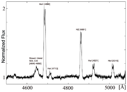
(a) The normalized and averaged spectra constructed from 140 individual exposures obtained at the VLT telescope.

(b) The flux-calibrated average of 200 spectrum observed with the Magellan telescope.

Figure 1:

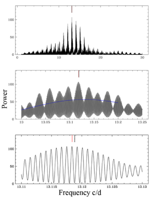
Figure 2: Power spectrum of the HeII radial-velocity data, obtained from the combined VLT and Magellan data sets. The vertical grey line in the bottom panel represents the best period found by Patterson et al. 1998, along with its error. The red line represents the recalculated period using the latest photometric ephemeris (see Section 3.2.1) where the period derivative has been taken into account (Patterson et al. in preparation).

3.2 The Orbital Period

3.2.1 The Photometric Ephemeris

The key goal of our study is to obtain a definitive determination of T Pyx’s orbital period based on time-resolved spectroscopy. More specifically, we wish to test if the photometric modulation reported by Patterson et al. (1998) is orbital in nature. The photometric ephemeris is given by Patterson et al. (1998) as

Minimum light = HJD $2446439.428+0.0762233E+3.5\times 10^{-11}E^{2}$.

The quadratic term is highly significant and indicates a very high period derivative of $\dot{P}\simeq 9\times 10^{-10}$ (this corrects a typo in the original paper). The period is found to be increasing, which is not expected for a system that has not yet passed the minimum period. If the photometric signal is orbital, the current evolutionary time-scale of the system is only $\tau\sim P/\dot{P}\sim 3\times 10^{5}$ yrs. Such a short period change time-scale is highly unusual for a CV.

The Center for Backyard Astronomy (CBA) has continued to gather additional timings in the period 1996 – 2009. This new photometry, along with an updated ephemeris, will be published in due course (Patterson et al., in preparation). However, since this new data set is much more suited to a comparison against our spectroscopic observations (since it overlaps in time), Joe Patterson has kindly made this latest set of CBA timings available to us. Our own prelimary analysis of all the existing timings yields a photometric ephemeris of

Minimum light = HJD(UTC) $2451651.65255(35)+0.076227249E(16)+2.546(54)\times 10^{-11}E^{2}$.

The numbers in parenthesis are the uncertainties on the two least significant digits, and were estimated via bootstrap simulations. Taking the period change into account, the average period at the time of the optical spectroscopy was $P=0.076228860\pm 3.0\times 10^{-8}$ d (corresponding to $f=13.1183912\pm 5.2\times 10^{-6}$ c/d).

This new ephemeris confirms that the period continues to increase at a fast rate. More specifically, the current estimate of the period derivative is $\dot{P}=(6.68\pm 0.14)\times 10^{-10}$, corresponding to a timescale of $P/\dot{P}\simeq 3\times 10^{5}$ yrs. It is important to take this period derivative into account when comparing spectroscopic and photometric periods.

3.2.2 The Spectroscopic Period

In order to establish the orbital period spectroscopically, we carried out a radial-velocity study using the double-Gaussian method (Schneider & Young, 1980). This method is most effective in the line wings, which are formed in the inner regions of the accretion disc. As discussed further in Section 3.4, we tried a variety of Gaussian FWHM’s, as well as a range of separations between the two Gaussians.

The results shown in this section are for a FWHM = 450 km s^-1 and a separation of 300 km s^-1, and are based on the full combined VLT + Magellan data set, spanning the time period December 2004 to March 2008. The radial-velocity study was carried out for several spectral lines but for the purpose of this section, we will focus exclusively on the radial-velocities derived from the strong HeII line at 4686 Å, since this line provides the most accurate results. The power spectrum (Scargle, 1982) of this spectroscopic data set is presented in Figure 2. The top panel, covering a broad frequency range, confirms that there is a strong signal near the photometrically predicted 13 c/d. No signal is found at $P=3.44$ hours, corresponding to the period found by Vogt et al. (1990). The middle and bottom panels show close-ups of narrower frequency ranges around this power spectral peak. Note, in particular, that the red line in the bottom panel marks the photometrically predicted frequency for the epoch corresponding to the mid-point of our spectroscopic data set. For comparison, we also show the frequency of the linear ephemeris determined by Patterson et al. (1998) for just the 1996-1997 timings, along with its error. The spectroscopic and photometric periods appear to be mutually consistent, but only if we account for the photometry period derivative. More specifically, the $\dot{P}$-corrected photometric prediction lies extremely close to the peak of the most probable spectroscopic alias.

This apparent consistency can be checked more quantitatively. The orbital frequency predicted by the photometry for the average epoch of our spectroscopy is $f_{phot}=13.1183912\pm 5.2\times 10^{-6}$ c/d, where the error is once again based on bootstrap simulations. Similarly, we have carried out a bootstrap error analysis for the frequency determined from our spectroscopy. Since we are only interested in the agreement between the photometry and the spectroscopy, we only considered the spectroscopic alias closest to the photometrically determined frequency (this is also the highest alias). This yielded $f_{spec}=13.118368\pm 1.1\times 10^{-5}$ c/d. The difference between these determinations formally amounts to just under 2$\sigma$. We consider this to be acceptable agreement.

The level of agreement between spectroscopic and photometric periods is important. The spectroscopy on its own is sufficient to establish beyond doubt that T Pyx is a short-period system with $P_{orb}\simeq 1.8$ hrs. However, the fact that we can establish reasonable consistency with the photometric data if (and only if) we account for the photometric period derivative suggests that (i) we can trust the much higher precision photometric data to provide us with the most accurate estimate of the orbital period, and (ii) that the large period derivative suggested by the photometry is, in fact, correct.

3.3 Trailed Spectrograms and Doppler Tomography

In order to visualize the orbital behavior of the spectral profiles, trailed spectrograms were constructed for HeII, HeI, H$\beta$ and the Bowen blend. These spectrograms, shown in Figure 3, are phase binned to match the orbital resolution of our data (37 bins for the VLT data and 27 bins for the Magellan data), and are here plotted over 2 periods. All lines show emission features moving from the blue to the red wing, and localized emission is seen in the red wing at phase, $\phi\approx 0.6$. Similar structures are seen in the spectrograms for both the HeII and the Bowen blend indicating that they originate in the same line-forming region, presumably the accretion disc.

Doppler tomography (Marsh & Horne, 1988), is an indirect imaging method where the emission-line profiles, depending on phase, are plotted onto a velocity scale. The method was used to visualize, in velocity space, the origin of the emission features found in T Pyx. In Figure 4, Doppler tomograms for the most prominent lines are presented. For the reconstruction of the tomograms, the systemic velocity, $\gamma$ was set to zero (see Section 3.4.1). All lines show asymmetrically distributed emission from the disc. These asymmetric features are also seen in the trailed spectrograms (Figure 3). No emission can be connected to the bright spot, the accretion stream or the donor star. The map of the Bowen blend was constructed from a composite of the three lines, NIII at $\lambda$4640.64 and CIII at $\lambda$4650.1 and $\lambda$4647.4.

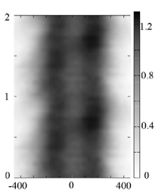
(a) Magellan, HeII(4686)

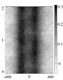
(b) Magellan, HeI(4921)

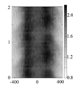
(c) VLT, HeII(4686)

(d) VLT, H$\beta$(4861)

Figure 3: Trailed spectrograms, phase binned to match the orbital resolution (37 bins for the VLT data and 27 bins for the Magellan data), are here plotted over 2 periods. Phases are plotted against velocities (in km s^-1).

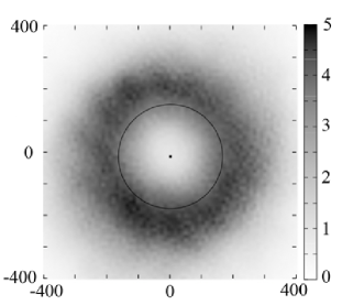
(a) Magellan, HeII(4686)

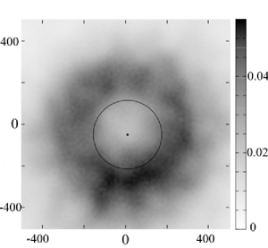
(b) Magellan, Bowen blend NIII(4641) and CIII(4650, 4647)

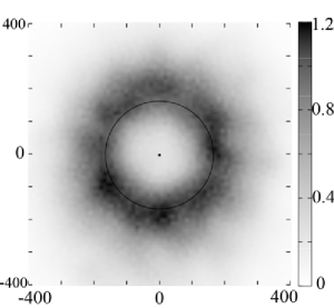
(c) Magellan, HeI(4921)

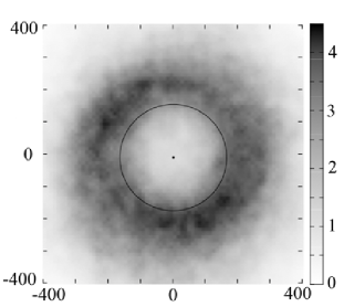
(d) VLT, HeII(4686)

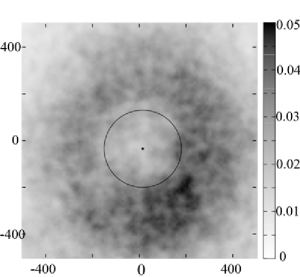
(e) VLT, Bowen blend NIII(4641) and CIII(4650, 4647)

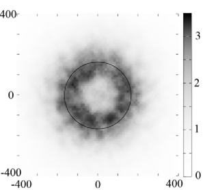
(f) VLT, H$\beta$(4861)

Figure 4: Doppler tomograms for the most prominent lines. The center of symmetry in each map is marked as a dot and the outer disc radius is plotted as a circle. Both axis are in km s^-1.

3.4 A Radial-Velocity Study of T Pyx

3.4.1 The Systemic Velocity

We noticed early on in our analysis for both the VLT and Magellan data sets that the systemic velocity, $\gamma$, appeared to be varying with time. In order to confirm the reality of these variations, we extracted spectra from a few VLT/GIRAFFE/FLAMES fibres that were centered on knots in the nova shell surrounding T Pyx. The intrinsic radial velocities of these large-scale knots are not expected to change appreciably over a time-scale of months, so they provide a useful check on the stability of our wavelength calibration. We found that the shifts seen in the radial velocity data for the central object are much larger than those seen for the knots, suggesting that these shifts cannot be explained by instrumental effects alone. However, since we have only five nights worth of VLT data spread over two months, our data set is too sparse to allow a careful study of trends in the apparent $\gamma$ velocities. For the purpose of the present study, we thus subtracted the mean nightly $\gamma$ from all radial velocities before carrying out any analysis. This should minimize the risk of biasing our results.

3.4.2 The Velocity Semi-Amplitude

In order to establish the velocity semi-amplitude, $K1$, of the WD, further analysis was pursued on the radial-velocity data obtained from the double-Gaussian method. A least squares fit was made to the radial velocity curves by keeping the orbital period fixed, but allowing the three parameters, the systemic velocity, $\gamma$, the velocity semi-amplitude, $K$, and the phase, $\phi_{0}$, to vary. Phase zero corresponds to the photometric phase minimum light. The errors on the input radial velocity data, provided in MOLLY, were used to calculate the $\chi^{2}$ and then rescaled so that $\chi^{2}=1$. The technique was applied to several strong lines in both the VLT and Magellan data sets, but the radial velocity data measured from the HeII line at 4686 Å, and in particular from the Magellan dataset, gave the most reliable fits. The results were plotted in a diagnostic diagram (see Shafter, 1983; Thorstensen, 1986 and Horne, Wade, & Szkody, 1986). However, as can be seen in Figure 5, the key parameters ($\gamma$, $K$ and $\phi_{0}$) did not converge convincingly for any combination of the FWHM and separation. Normally, it is thought that the bright spot or other asymmetries in the disc are responsible for distorting the diagnostic diagram. However, in T Pyx the disc appears to be rather symmetric, and no contribution from the bright spot is seen (see Figure 4). We conclude that the radial velocity curves obtained from the double-Gaussian method are, most likely, not tracking the velocity of the primary WD, and therefore, $K1$, and $\phi_{0}$ cannot be estimated reliably using this method.

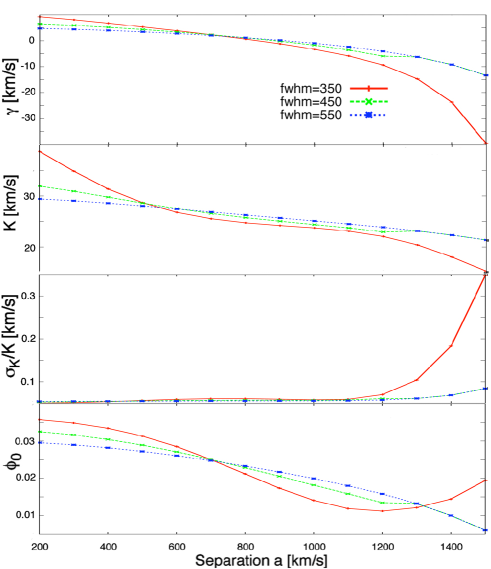
Figure 5: Diagnostic diagram for the HeII line, Magellan. None of the parameters ($\gamma$, $K$ and $\phi_{0}$) are converging for any combination of the FWHM and separation.

In order to improve on the results obtained from the double-Gaussian method, we used two other techniques to obtain an estimate of $K1$. First, we measured the velocity center of the lines by fitting Gaussians to the individual spectral lines. Two Gaussians were fitted to the double-peaked lines, keeping the FWHM and the rest wavelength of the line fixed, but allowing the peak offsets and the peak strengths to vary. Radial velocity curves were then plotted for both blue and red wings. As can be seen from the trailed spectrograms, Figure 3, the red wing (in particular for the HeII lines) does not show the same smooth orbital signal as the blue wing. Consequently, only the data from the blue wing was taken into account when measuring $K1$. Several lines from both the VLT and Magellan data sets were analyzed. The data were phase-binned to the orbital resolution, velocity-binned in a $\sim$ 100 pixel wide region around the line, and the nightly mean $\gamma$ was subtracted. HeII at $\lambda$4686 is the strongest line and was ultimately used to estimate our best-bet value of the velocity semi-amplitude of the WD: $K1=17.9\pm 1.6$ km s^-1. Figure 6 shows the radial velocities obtained for the HeII line in the Magellan data set. Data presented in black are phase-binned to the orbital resolution afforded by our time-resolved spectroscopy, while all invidual data points are shown in grey. Over-plotted onto the radial velocity curve is the best sinusoidal fit, indicating a phasing close to zero, $\phi_{0}=-0.03\pm 0.03$. Figure 7 shows the final trailed spectrograms from the HeII at $\lambda$4686 in the Magellan data set that was used to determine $K1$.

Second, $K1$ can also be measured from the Doppler tomograms, by locating the center of symmetry of the disk emission that dominates the maps. This center should be located at $V_{x}=0$ and $V_{y}=-K1$ (eg. Steeghs & Casares, 2002). After masking out any regions of strong asymmetric non-disk emission, the center of symmetry was found by taking a trial point, smoothing the map azimuthally about this point, and then subtracting this smoothed map from the real map. If the trial point is far from the center of symmetry, the resulting difference map will contain large asymmetric residuals. The optimal center of symmetry is thus the trial point for which the difference map exhibits the smallest residuals (as measured by the standard deviation of the difference map). This procedure yielded estimates for $K1$ that were consistent with those obtained from the Gaussian fits ($14<K1<19$ km s^-1). We thus adopt $K1=17.9\pm 1.6$ km$\,s^{-1}$ as our best-bet estimate.

In closing this section, it should be acknowledged that our final estimate of $K1$ is subject to considerably systematic uncertainties. In particular, it is difficult to rule out that whatever is preventing the double Gaussian method from converging may also bias the Gaussian fits to the line peaks and the center of symmetry of the tomograms. Strictly speaking, our estimate of $K1$ should thus perhaps be viewed as a lower limit. However, we are reasonably confident that our measurements do trace the orbital motion of the WD in T Pyx. This is mainly because the presence of persistent double-peaked lines and ring-like structure in the tomograms implies that there is a strong accretion disk component to the line emission. This disk component must ultimately trace the motion of the WD, and our two preferred methods are designed to exploit this in as direct a fashion as possible, while simultaneously minimizing contamination from asymmetrically placed emission regions.

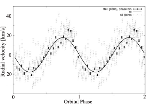
Figure 6: Radial velocity curve of the HeII line, Magellan. Data in black is phase binned while all data are shown in grey. The best sin fit is over-plotted onto the phase-binned data.

3.4.3 The Velocity at the Outer Disc Radius

The peak-to-peak separations of the double peaked emission lines can be used to estimate the projected velocity at the outer disc radius, $v(R_{disk})\sin i$. We thus fitted Gaussians to the phase-binned, double-peaked H$\beta$, HeI and HeII lines in the Magellan data set. The peak-to-peak separations varies significantly with line but the mean value is close to that for HeI. We therefore use the HeI peak-to-peak separation for our estimation of $v(R_{disk})\sin i$, and adopt half the full range as a rough estimate of the associated error, $\Delta V_{peak-to-peak}=290\,\pm\,26$ km s^-1.  Smak (1981) investigated the exact relationship between the true $v(R_{disk})\sin i$ and the measured $\Delta V_{peak-to-peak}$, taking into account the effects of instrumental broadenings and different disk emissivity distributions. He found that, for a wide range of parameters, $v(R_{disk})\sin i=0.5\Delta V_{peak-to-peak}/u$, where $u=1.05\,\pm\,0.05$. Taking this into account, we find $v(R_{disk})\sin i=138\pm 15$ km s^-1.

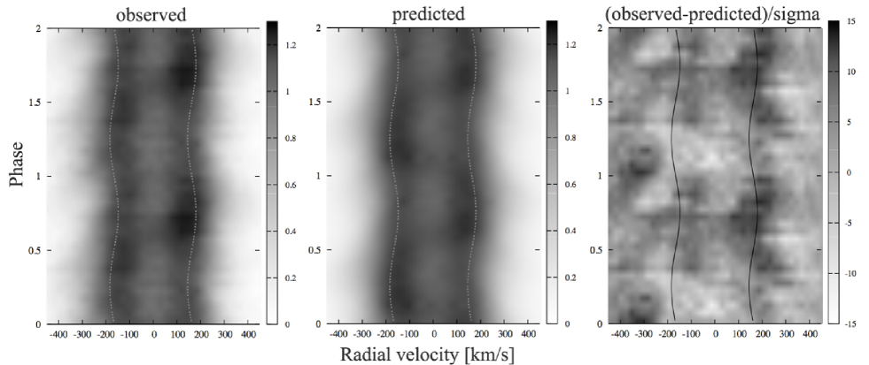
Figure 7: Trailed spectrograms for the HeII line, Magellan.

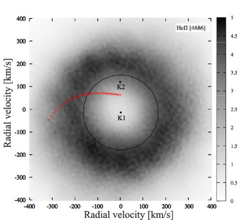
Figure 8: Doppler tomogram for the HeII line, Magellan. The location of the WD, $K1$, the outer disc radius as well as the location of the donor star, $K2$, and the accretion stream is plotted onto the map.

4 Spectroscopic System Parameters

If we are willing to assume that our estimates of $K1$ and $v(R_{disk})\sin i$ are valid, we can use our data to estimate several other system parameters.

4.1 Mass Ratio

The method we use to estimate the mass ratio, $q$, is similar to that described in Warner (1973). The basic idea is that, subject to fairly benign assumption, the ratio $v(R_{disk})\sin i/K_{1}$ should be a function of only $q$. More specifically, we assume that the disk is circular, Keplerian, and, since T Pyx is a high-$\dot{M}$ system, that it extends all the way to the tidal radius. The disk radius can then be taken as $R_{disk}/a=0.60/(1+q)$ (Warner, 1995). These assumptions, together with Kepler’s third law, yield the expected relationship

$$\frac{v(R_{disk})\sin i}{K1}=1.2909\frac{1+q}{q}$$ (1)

Using this expression, we estimate a mass ratio of $q=0.20\pm 0.03$.

Given a mass ratio and disk radius, it is possible to estimate the expected phasing of the bright spot in the system, if we make the usual assumption that the bright spot lies at the point where the ballistic accretion stream from the L₁ point meets the disk edge (see, for example, Patterson, Thorstensen & Knigge, 2008; Patterson et al., 2000). Carrying out this calculation for T Pyx suggests that the bright spot could be located at orbital phase $\phi\simeq-0.03$. This is interesting, because it is consistent with the negligible phase offset we have found between photometric minimum light and the red-to-blue crossing of the WD radial velocity curve. Thus, based on phasing alone, the bright spot could be the source of the photometric modulation. However, there are also other interpretations for the photometric signature. For example, the orbital signal could be dominated by a reflection effect, i.e. the changing projected area of the irradiated face of the donor as it moves around the orbit. This would explain why inferior conjunction of the secondary corresponds to minimum light. On the other hand, it raises the question why we do not see the signature of the irradiated donor in our spectroscopy. As noted above, there is no sign of the narrow Bowen fluorescence lines that one might expect in the case of strong donor irradiation.

4.2 Component Masses

Recurrent novae are expected to harbor a more massive WD than most ordinary CVs, and even than most classical novae. In a classical nova, the mass of the WD is typically close to 1 M_⊙, both theoretically and observationally. Based on this, both Selvelli et al. (2008) and  Schaefer, Pagnotta & Shara (2009) agree on a plausible mass range for the primary WD in T Pyx of 1.25 $-$ 1.4 M_⊙ (using theoretical models by Yaron et al., 2005). From the theoretical point of view, a high-mass WD is needed to achieve a sufficiently short outburst recurrence timescale.

In T Pyx, the bright accretion disc outshines any spectral signature from the donor star, and we can therefore not constrain the donor mass spectroscopically. However, we can use the period-density relation for Roche-lobe filling secondary stars (Eggleton, 1983) to set some constraints.

As shown by Patterson, Thorstensen & Kemp (2005) and Knigge (2006), the donor stars in ordinary CVs below the period gap are inflated by approximately 10% due to mass loss, relative to ordinary main sequence stars of the same mass. Given T Pyx’s peculiar evolutionary state, it is not clear if this level of inflation is appropriate for T Pyx, and we therefore adopt a conservative range of 0% $-$ 20% inflation. In order to estimate the mass of the donor star, we thus take the theoretical main-sequence mass-radius relation from the 5 Gyr isochrone of Baraffe et al. (1998), adjust the stellar radius to account for inflation, and then find the secondary mass that yields the correct density for T Pyx’s orbital period. This yields $M_{2}=0.14\pm 0.03$ M_⊙. Note that the inferred donor mass decreases with increasing levels of radius inflation. The corresponding mass of the WD is then $M_{1}=0.7\pm 0.2\,$M_⊙.

Since this estimate of the WD mass is lower than expected for a recurrent nova, we can also turn the problem around. If the mass of the WD is $>1$ M_⊙, as theoretical nova models imply (Yaron et al., 2005), the mass of the donor becomes > $0.2\,$M_⊙, if our estimate of the mass ratio is correct.

All of these estimates should, of course, be taken with a grain of salt. In particular, they rely on (i) the correctness of our measured $K1$ and (ii) the assumption that the disk extends all the way to the tidal radius. Despite these uncertainties, our calculations highlight an important point: it is highly unlikely that the donor star in T Pyx is already a brown dwarf. For example, if we retain the assumption of maximal disk size, $K1\leq 7$ km s^-1 would be required in order for $M_{2}\leq 0.07$ M_⊙ for any $M_{1}>1\leavevmode\nobreak\$M_⊙. We thus rule out the possibility that T Pyx is a period bouncer in the usual sense, i.e. that it had already reached the minimum period for ordinary CVs ($\simeq 70$ min theoretically, or $\simeq 80$ min observationally), in which case its secondary would now be well below the Hydrogen-burning limit.

4.3 The Orbital Inclination

The orbital inclination for T Pyx is thought to be low due to the sharp spectral profiles and low radial velocity amplitude. Shahbaz et al. (1997) suggested a lower limit of the orbital inclination for T Pyx of $i\sim 6^{\circ}$ based on the peak-to-peak separation of the H$\alpha$ line in their spectra. Patterson et al. (1998) estimated an inclination of $i\sim 10^{\circ}-20^{\circ}$ due to the low amplitude of the orbital signal, and Selvelli et al. (2008) estimated $i\sim 20^{\circ}-30^{\circ}$.

The inclination, $i$, can be estimated from our data via $K1=v_{1}\sin i$, where $v_{1}=(2\pi a)/P\times(q/(q+1))$ and $a$ is the distance between the two components obtained from Kepler’s III law. This provides a constraint on the system inclination of $i=10\pm 2$ degrees, for any reasonable combination of the component masses. We stress that the real uncertainty on the inclination is bound to be larger, because the formal error does not include systematic uncertainties associated with, for example, possible bias in our $K1$ measurement and the assumption of tidal truncation in our derivation of $q$.

5 Summary and Discussion

The main result of our study is the spectroscopic determination of T Pyx’s orbital period, $P_{orb}\simeq 1.83$ hrs. This confirms that the system is a CV below the period gap and implies that its current accretion rate is at least 2 orders of magnitude higher than that of an ordinary CV at this period. We also find that our spectroscopic orbital period is consistent with the photometric ephemeris found for T Pyx (Patterson et al., 1998, an updated version is given in Section 3.2.1). This means not only that photometric timings can be used as a more precise and convenient tracer of the orbital motion, but also that the large period derivative required by the photometric ephemeris marks a genuine change in the orbital period of the system. In fact, the spectroscopic data are consistent with the photometric period only if the period derivative is accounted for. The period derivative obtained here from the latest combined photometric data ($\dot{P}=6.7\times 10^{-10}$) is slightly lower than that obtained by Patterson et al. (1998) from data up to 1997 ($\dot{P}\simeq 9\times 10^{-10}$). A decrease in the rate of period change would be in line with Schaefer, Pagnotta & Shara (2009) scenario that T Pyx’s days as a high-$\dot{M}$ recurrent nova are numbered (at least until its next ordinary nova eruption). In any case, the average time-scale for period change found across all the photometric data are about $3\times 10^{5}$ yrs.

We have also used our spectroscopic data to obtain estimates of other key system parameters, most notably the radial velocity semi-amplitude of the WD, $K1=17.9\pm 1.6$ km s^-1, and the mass ratio, $q=0.20\pm 0.03$. The latter estimate rests on three key assumptions: first, that our determination of $K1$ is correct, second, that our estimate $v(R_{disk})\sin i$ is correct, and, third, that the accretion disk around the WD in T Pyx is tidally limited. Taken at face value, this relatively high value of the mass ratio implies that the donor star in the system is not a brown dwarf. Thus T Pyx is not a period bouncer. If we assume that the radius of the secondary is $10\%\pm 10\%$ inflated relative to an ordinary main sequence star of the same mass, we find that its most likely mass is $M_{2}=0.14\pm 0.03$ M_⊙.

Overall, the physical picture that emerges from our study is consistent with the scenario proposed by Schaefer, Pagnotta & Shara (2009). In particular, they suggest that, prior to the 1866 eruption, T Pyx was an ordinary CV. That eruption then triggered a high-$\dot{M}$ wind-driven phase, as suggested by Knigge, King & Patterson (2000) to account for T Pyx’s exceptional luminosity. However, this phase is not quite self-sustaining, so that T Pyx is now fading and perhaps not even a RN anymore. In line with this picture, we find that the mass ratio and donor mass we derive are not abnormally low for a CV at its orbital period. This shows that the present phase of high-$\dot{M}$ accretion cannot have gone on for too long already. The hint of a declining period derivative may point in the same direction, but this needs to be confirmed.

Does all this mean that the phase of extraordinarily high accretion rates T Pyx is currently experiencing will have no lasting impact on its evolution? Not necessarily. In a stationary Roche-lobe-filling system, the orbital period derivative and total mass-loss rate from the donor (wind loss + mass transfer) are related via

$$\frac{\dot{P}_{orb}}{P_{orb}}=\frac{3\zeta-1}{2}\frac{\dot{M}_{2}}{M_{2}}$$ (2)

where $\zeta$ is the donor’s mass-radius index. In T Pyx, which has an increasing orbital period, we will take $\zeta\simeq-1/3$, which is appropriate for adiabatic mass-loss from a fully convective star (e.g. Knigge, King & Patterson, 2000). We thus expect that $\dot{M_{2}}/M_{2}\simeq{\dot{P}_{orb}}/{P_{orb}}$, which suggests a typical mass-loss rate from the donor of $\dot{M_{2}}\sim 5\times 10^{-7}$ M_⊙/yr in its current state. (The accretion rate onto the WD can be lower than this, since, in the wind-driven scenario, much of this mass escapes in the form of an irradiation-driven outflow from the donor.) If every ordinary nova eruption in T Pyx is followed by $\sim$ 100 yrs of such high-$\dot{M}_{2}$ evolution, the total mass loss from the donor in the luminous phase is $\sim 5\times 10^{-5}$ M_⊙ between any two such eruptions. This needs to be compared to the mass lost from the donor during the remaining part of the cycle. If this is driven by gravitational radiation, the mass loss rate from the donor will be $\dot{M}_{2}\simeq 5\times 10^{-11}$ M_⊙/yr (Knigge, King & Patterson, 2000). The recurrence time of ordinary nova eruptions for such a system is on the order of $10^{5}$ yrs (Yaron et al., 2005), so the total mass lost from the donor during its normal evolution (outside the wind-driven phase) is $5\times 10^{-6}$ M_⊙. This shows that the long-term secular evolution may be dominated by its high-$\dot{M}$ wind-driven phases, even if the duty cycle of these phases is very low (e.g. 0.1% for the numbers adopted above).

It is finally tempting to speculate on the relevance of “T Pyx-like” evolution for ordinary CVs. At first sight, the numbers above suggest that the evolution of a CV caught in such a state may be accelerated by about an order of magnitude. This is interesting, since it could bear on the long-standing problem that there are fewer short-period CVs and period bouncers in current samples than theoretically expected (e.g. Patterson et al., 1998; Pretorius, Knigge & Kolb, 2007; Pretorius et al., 2007; Pretorius & Knigge 2008ab). Moreover, this channel need not be limited to systems containing high-mass WDs that are capable of becoming RNe. After all, it is not the recurrent nova outbursts that are of interest from an evolutionary point of view, but simply the existence of a prolonged high-$\dot{M}$ phase in the aftermath of nova eruptions. In CVs containing lower-mass WDs, such a phase may still occur, although its evolutionary significance could still depend on the WD mass. For example, the interoutburst time-scale is longer for low-mass WDs, and the duration of the high-$\dot{M}$ phase could also scale with WD mass. One obvious objection to this idea is that, observationally, most nova eruptions are not followed by centuries- (or even decades-) long high-$\dot{M}$ phases. However, this need not be a serious issue. Most observed novae are long-period systems, so if the triggering of a wind-driven phase requires a fully convective donor, most novae would not be expected to enter such a phase. It may be relevant in this context that at least one other short-period nova – GQ Mus – exhibited an exceptionally long post-outburst supersoft phase of $\sim 10$ years (Oegelman et al., 1993). Greiner et al. (2003) have also suggested that the duration of the supersoft phase in novae may scale inversely with orbital period.

However, there is another important consequence to the idea that the evolution of many short-period CVs is accelerated by “T Pyx-like” high-luminosity phases. The orbital period-derivative is positive in the high-$\dot{M}$ phase, but negative during the remaining times of GR-driven evolution. But since $\dot{P}_{orb}/P_{orb}\simeq\dot{M}_{2}/M_{2}$ in both phases, the sign of the secular (long-term-average) period derivative will generally correspond to the phase that dominates the secular evolution. So whenever wind-driving dramatically accelerates the binary evolution, the direction of period evolution will also be reversed. Is this a problem? Perhaps. The recent detection of the long-sought period spike in the distribution of CV orbital periods (Gänsicke et al., 2009) suggests that there is, in fact, a reasonably well-defined minimum period for CVs, as has long been predicted by the standard model of CV evolution (e.g. Kolb, 1993). On the other hand, the location of the observed spike ($\simeq 83$ mins) is significantly different from the expected one ($\simeq 65-70$ min). Is it possible that the observed period minimum corresponds to the onset of wind-driving in most CVs? T Pyx, with $P_{orb}\simeq 110$ min would then have to be an outlier, however, perhaps because of an unusually high WD mass.

The idea that T Pyx-like phases may significantly affect the evolution of many CVs is, of course, highly speculative, and we do not mean to endorse it too strongly. However, it highlights the importance of understanding T Pyx: until we know what triggered the current high-luminosity state, it will remain difficult to assess the broader evolutionary significance of this phase. Note that the apparent uniqueness of T Pyx is not a strong argument against such significance. For example, if the duty cycle of high-luminosity phases is $\sim 0.1$%, as suggested by the numbers above, we should not expect to catch many CVs in this state. Thus T Pyx could be the tip of the proverbial iceberg.

References

- Baraffe et al. (1998) Baraffe, I., Chabrier, G., Allard, F., et al. 1998, A&A, 337, 403
- Eggleton (1983) Eggleton, P. P. 1983, ASSL, 101, 39
- Greiner et al. (2003) Greiner, J., Orio, M. & Schartel, N. 2003, A&A, 405, 703
- Gänsicke et al. (2009) Gänsicke, B. T., Dillon, M., Southworth, J., et al. 2009, MNRAS, 397, 2170
- Hamuy, et al. (1992) Hamuy, M., Walker, A.R., Suntzeff, N.B., et al. 1992, PASP, 104, 533
- Horne, Wade, & Szkody (1986) Horne, K., Wade, R. A., & Szkody, P. 1986, MNRAS, 219, 791
- Knigge, King & Patterson (2000) Knigge, C., King, A.R., & Patterson, J. 2000, A&A, 364, 75
- Knigge (2006) Knigge, C. 2006, MNRAS, 373, 484
- Kolb (1993) Kolb, U. 1993, A&A, 271, 149
- Margon & Deutsch (1998) Margon, B., & Deutsch, E.W. 1998, ApJ, 498, 61
- Marsh & Horne (1988) Marsh, T. R., & Horne, K. 1988, MNRAS, 235, 269
- Mennickent (1999) Mennickent, R. E. 1999, A&A, 348, 364
- Oegelman et al. (1993) Oegelman, H., Orio, M., Krautter, J., et al. 1993, Natur, 361, 331
- Patterson et al. (1998) Patterson, J., Kemp, J., Shambrook, A., et al. 1998, PASP, 110, 380
- Patterson et al. (2000) Patterson, J., Vanmunster, T., Skillman, David R., et al. 2000, PASP, 112, 1584
- Patterson, Thorstensen & Kemp (2005) Patterson, J, Thorstensen, J R. & Kemp, J. 2005, PASP, 117, 427
- Patterson, Thorstensen & Knigge (2008) Patterson, J., Thorstensen, J. R., Knigge, C. 2008, PASP, 120, 510
- Pretorius, Knigge & Kolb (2007) Pretorius, M. L., Knigge, C. & Kolb, U. 2007, MNRAS, 374, 1495
- Pretorius et al. (2007) Pretorius, M. L., Knigge, C., O’Donoghue, D., et al. 2007, MNRAS, 382, 1279
- Pretorius & Knigge (2008a) Pretorius, M. L., Knigge, C. 2008a, MNRAS, 385, 1471
- Pretorius & Knigge (2008b) Pretorius, M. L., Knigge, C. 2008b, MNRAS, 385, 1485
- Scargle (1982) Scargle, J. D. 1982, ApJ, 263, 835
- Schaefer, Pagnotta & Shara (2009) Schaefer, B.E., Pagnotta, A., & Shara, M. 2009, arxiv.org, 0906.0933
- Schneider & Young (1980) Schneider, D.P. & Young, P. 1980, ApJ, 240, 871
- Selvelli et al. (2008) Selvelli, P., Cassatella, A., Gilmozzi, R., et al. 2008, A&A, 492, 787
- Shafter (1983) Shafter, A. W. 1983, ApJ, 267, 222
- Shahbaz et al. (1997) Shahbaz, T., Livio, M., Southwell, K. A., et al. 1997, ApJ, 484, 59
- Smak (1981) Smak, J. 1981, AcA, 31, 395
- Steeghs & Casares (2002) Steeghs, D., & Casares, J. 2002, ApJ, 568, 273
- Thorstensen (1986) Thorstensen, J. R. 1986, AJ, 91, 940
- Vogt et al. (1990) Vogt, N., Barrera, L.H., Barwig,H., et al. 1990, Proc. of the 11th American Workshop on CV’s and LMXRB’s, Santa Fe, USA, Oct. 1989, etd. C.Mauche, Cambridge University Press, 391
- Warner (1973) Warner, B. 1973, MNRAS, 162, 189
- Warner (1995) Warner, B. 1995, Cataclysmic Variable Stars. Cambridge Univ. Press, Cambridge
- Williams (1982) Williams, R. E. 1982, ApJ, 261, 170
- Yaron et al. (2000) Yaron, R., Radebaugh, R., & Elias, E. 2000, ASAJ, 107, 2795
- Yaron et al. (2005) Yaron, O., Prialnik, D., Shara, M.M., et al. 2005, ApJ, 623, 398