Formation of Compact Stellar Clusters by High-Redshift Galaxy Outflows I: Nonequillibrium Coolant Formation

Abstract

We use high-resolution three-dimensional adaptive mesh refinement simulations to investigate the interaction of high-redshift galaxy outflows with low-mass virialized clouds of primordial composition. While atomic cooling allows star formation in objects with virial temperatures above $10^{4}$ K, “minihaloes” below this threshold are generally unable to form stars by themselves. However, these objects are highly susceptible to triggered star formation, induced by outflows from neighboring high-redshift starburst galaxies. Here we conduct a study of these interactions, focusing on cooling through non-equilibrium molecular hydrogen (H₂) and hydrogen deuteride (HD) formation. Tracking the non-equilibrium chemistry and cooling of 14 species and including the presence of a dissociating background, we show that shock interactions can transform minihaloes into extremely compact clusters of coeval stars. Furthermore, these clusters are all less than $\approx 10^{6}M_{\odot},$ and they are ejected from their parent dark matter halos: properties that are remarkably similar to those of the old population of globular clusters.

1. Introduction

A generic prediction of the cold dark matter model is a large high-redshift population of gravitationally-bound clouds that are unable to form stars. Because atomic H and He line cooling is only effective at temperatures above $10^{4}$ K, clouds of gas and dark matter with virial temperatures below this threshold must radiate energy through dust and molecular line emission. While the levels of H₂ left over from recombination are sufficient to cool gas in the earliest structures (e.g. Abel et al. 2002; Bromm et al. 2002), the resulting 11.20 - 13.6 eV background emission from the stars in these objects (e.g. Haiman et al. 1997; Ciardi et al. 2000; Sokasian et al. 2004; O’Shea & Norman 2007) is likely to have quickly dissociated these trace levels of primordial molecules (Galli & Palla 1998). And although an early X-ray background could have provided enough free electrons to promote H₂ formation, the relative strength between these two backgrounds is uncertain, and it is unlikely that the background was strong enough to balance ultraviolet (UV) photodissociation. Even if there were some trace amount of H₂ in these clouds, it is likely to be in such a small abundance as to not impact their structure (Whalen et al. 2008a; Ahn et al. 2009).

The result is a large number of dark matter halos that were massive enough to overcome the thermal pressure of the primordial intergalactic medium and retain their gas, but not massive enough to excite the radiative transitions necessary to cool this gas into stars. These “minihalos,” whose virial temperatures were $T_{\rm{vir}}\mathrel{\hbox{\hbox to0.0pt{\hbox{\lower 4.0pt\hbox{$\sim$}}\hss}\hbox{$<$}}}10^{4}$ K and whose total masses were between $10^{4}$ and $10^{7.5}M_{\odot}$ would have remained sterile until some outside force either disrupted them, or more interestingly, disturbed them so as to catalyze coolant formation. In fact, two possible coolant formation methods have been considered in detail in the literature: ionization fronts and shock fronts.

In the case of ionization fronts, such as would occur during the epoch of reionization, high-energy photons emitted from galaxies or quasars interact with the neutral atomic minihalo gas. Bond, Szalay & Silk (1988) originally discussed how the resulting photoionization would expel the gas contained in a minihalo by suddenly heating it to $T\approx 10^{4}$ K, as would be the case in the optically-thin limit. On the other hand, Cen (2001), used simple analytic estimates to argue that ionization fronts would cause non-equilibrium H₂ formation and the collapse of the gas inside the gravitational potential. However, Barkana & Loeb (1999) studied minihalo evaporation using static models of uniformly illuminated spherical clouds, accounting for optical depth and self-shielding effects, and showed that the cosmic UV background boiled most of the gas out of these objects. Later, Haiman, Abel, & Madau (2001) carried out three-dimensional (3D) hydrodynamic simulations assuming the minihalo gas was spontaneously heated to $10^{4}$ K, also finding quick disruption. Finally, full radiation-hydrodynamical simulations of ionization front-minihalo interactions were carried out in Iliev et al. (2005) and Shapiro et al. (2004; see also Shapiro, Raga & Mellema 1997; 1998). These demonstrated that intergalactic ionization fronts decelerated when they encountered the dense, neutral gas inside minihaloes and were thereby transformed into D-type fronts, preceded by shocks that completely photoevaporated the minihalo gas.

A second and more promising avenue for coolant formation is the interaction between galactic outflows and minihaloes. These galaxy-scale winds, which are driven by core-collapse supernova and winds from massive stars, are commonly observed around dwarf and massive starbursting galaxies at both low and high redshifts (e.g. Lehnert & Heckman 1996; Franx et al. 1997; Pettini et al. 1998; Martin 1999; 1998; Heckman et al. 2000; Veilleux et al. 2005; Rupke et al. 2005), and a variety of theoretical arguments suggest that these galaxies represent only the tail end of a larger population of smaller “pre-galactic,” starbursts that formed before reionization (Scannapieco, Ferrara & Madau 2002; Thacker, Scannapieco, & Davis 2002). Furthermore, the interstellar gas swept up in a starburst-driven wind can effectively trap the ionizing photons behind it (Fujita et al. 2003), meaning that at high redshifts, many intergalactic regions may have been impacted by outflows well before they were ionized.

Such $\approx 100-300$ km/s shocks can cause intense cooling through two mechanisms: (i) the mixing of metals with ionization potentials below 13.6 eV (Dalgarno & McCray 1972), which allow for atomic line cooling even at temperatures below $10^{4}$ K; and (ii) the formation of H₂ and HD by nonequilibrium processes (Mac Low & Shull 1986; Shapiro & Kang 1987; Kang et al. 1990; Ferrara 1998; Uehara & Inutsuka 2000), which allow for molecular line cooling associated vibrational and rotational transitions (Palla & Zinnecker 1988). In fact, Scannapieco et al. (2004) showed that these effects were so large that shock interactions could induce intense bursts of cooling and collapse in previously “sterile” minihalo gas. Using simple analytic models, they found that the most likely result was the formation of compact clusters of coeval stars, although they also emphasized the importance of multidimensional numerical studies to confirm this result.

In this paper, we present the first in a series of 3D numerical studies to capture the physical interactions between primordial minihalos and supernova-driven galactic outflows. While triggered star formation has been simulated in low-redshift intergalactic clouds impacted by radio jets (e.g. van Breugel et al. 1985; Fragile et al. 2004; Wiita 2004; Klamer et al. 20004), this has never been numerically simulated in the high-redshift, minihalo case. In this paper, we focus on the physics of non-equilibrium H₂ and HD chemistry and associated cooling in determining the properties of the post-shock minihalo gas. In particular, we show that molecule formation and the resulting cooling is strong enough to induce rapid minihalo collapse and star formation, leading to compact stellar clusters.

The structure of this paper is as follows. In §2 we outline the physical components of the model, focusing on our primordial H₂ and HD chemical network and cooling routines and their respective tests. In §3 we outline the general model used for the galactic outflow and the minihalo, and in §4 we present the simulation results and relate the resulting stellar clusters to local observations. Conclusions are given in §5.

2. Numerical Method

All simulations were performed with FLASH version 3.1, a multidimensional adaptive mesh refinement hydrodynamics code (Fryxell et al. 2000) that solves the Riemann problem on a Cartesian grid using a directionally-split Piecewise-Parabolic Method (PPM) solver (Colella & Woodward 1984; Colella & Glaz 1985; Fryxell, Müller, & Arnett 1989). Furthermore, unlike earlier versions of the code, FLASH3 includes an effective parallel multigrid gravity solver as described in Ricker (2008). However, before shock-minihalo interactions could be simulated, two capabilities needed to be added: nonequilibirum primordial chemistry, and cooling from atoms and from molecules produced in these interactions. In this section we describe our numerical implementation of each of these processes, along with the tests we carried out before applying the code to shock-minihalo interactions.

2.1. Chemistry

As the minihalos we are considering in this paper are made up of primordial gas, their chemical makeup is highly restricted, with contributions from only hydrogen, helium, and low levels of deuterium. Yet even these three isotopes can exist in a variety of ionization states and molecules and are thus associated with a substantial network of chemical reactions that must be tracked throughout our simulations.

2.1.1 Implementation

The chemical network that was implemented into FLASH is outlined by Glover & Abel (2008, hereafter GA08). Throughout our simulations we track three states of atomic hydrogen (H, H⁺, & H^-) and atomic deuterium (D, D⁺, & D^-), three states of atomic helium (He, He⁺, $\&$, He⁺⁺), two states of molecular hydrogen (H₂ $\&$ H${}_{2}^{+}$) and molecular hydrogen deuteride (HD $\&$ HD⁺), and electrons (e^-). For simplification, any reaction that involved molecular deuterium (D₂) and all three-body reactions were neglected. As stated in GA08, the very small amount of D₂ and D${}_{2}^{+}$ produced makes any cooling by these molecules irrelevant, while three-body reactions only become important at $n\mathrel{\hbox{\hbox to0.0pt{\hbox{\lower 4.0pt\hbox{$\sim$}}\hss}\hbox{$>$}}}10^{8}$ cm^-3 (e.g. Palla et al. 1983), many orders of magnitude denser than the conditions considered here. With these constraints, a total of 84 reactions were used out of the 115 described in GA08.

Photodissociation rates due to an external radiation field were also included as given in Glover & Savin (2009). These rates are calculated assuming a $T_{\rm eff}=10^{5}$ K blackbody source and their strength is quantified by the flux at the Lyman limit, $J(\nu_{\alpha})=10^{-21}J_{21}$ erg $\rm s^{-1}$ $\rm cm^{-2}$ $\rm Hz^{-1}$ $\rm sr^{-1}$. Note that once H₂ and HD are produced in sufficient quantities, some molecules are self-shielded from the background radiation. However, for simplicity, we considered only the case where there was no self-shielding, and thus our results place an upper limit on the effect of a dissociating background. This process adds an additional 7 reactions for a total of 91 reactions in the chemical network.

In reactions that involve free electrons recombining with ions, there are two possible choices for the reaction rate, depending on the overall optical depth of the cloud to ionizing radiation. In the optically-thin case (Case A; Osterbrock 1989) ionizing photons emitted during recombination are lost to the system, while in the optically-thick case (Case B), ionizing photons are reabsorbed by neighboring neutral atoms, which have the effect of lowering the recombination rates by essentially not allowing recombination to the ground state. There are three reactions (${\rm{H}}^{+}+{\rm e}^{-}\rightarrow{\rm H}+\gamma$, ${\rm He}^{+}+{\rm e}^{-}\rightarrow{\rm He}+\gamma$, and ${\rm He}^{++}+{\rm e}^{-}\rightarrow{\rm He}^{+}+\gamma$) where this is a concern, and as we shall see below, in all cases our clouds are optically thick, such that Case B recombination rates are appropriate.

The binding energy from each species is also important in the total energy budget and on the evolution of the gas. In FLASH these are defined such that all of the neutral species (H, D, e^-, & H) have binding energies equal to zero. As the gas is heated and the atomic species begin to ionize, the endothermic reactions remove the binding energy between the nucleus and electron(s) from the internal energy of the gas. For H and D this requires 13.6 eV, while the ionized states for Helium (He⁺ and He⁺⁺) have ionization potentals of 24.5 eV and 79.0 eV respectively. H^- and D^- are only weakly bound and have similar binding energies of 0.75 eV. Finally H₂ and HD have binding energies of 4.4 eV, and H${}_{2}^{+}$ and HD⁺ have binding energies of 10.9 eV, somewhat lower than the atomic species.

To describe the evolution of our 14 species, we enumerate them with an index $i$ such that each has $Z_{i}$ protons and $A_{i}$ nucleons, following the structure and syntax from Timmes (1999). Next we consider a gas with a total mass density $\rho$ and temperature $T$ and denote the number and mass densities of the $i$th isotope as $n_{i}$ and $\rho_{i},$ respectively. For each species we also define a mass fraction

$$X_{i}\equiv\rho_{i}/\rho=n_{i}A_{i}/(\rho N_{A}),$$ (1)

where $N_{A}$ is Avogadro’s number, and we define the molar abundance of the $i$th species as

$$Y_{i}\equiv X_{i}/A_{i}=n_{i}/(\rho N_{A}),$$ (2)

where conservation of mass is given by $\sum^{N}_{i}X_{i}=1.$ Each of the 14 species can then be cast as a continuity equation in the form

$$\dot{Y}_{i}\equiv\frac{dY_{i}}{dt}=\dot{R_{i}},$$ (3)

where $\dot{R_{i}}$ is the total reaction rate due to all the binary reactions of the form $i+j\rightarrow k+l,$ defined as

$$\dot{R_{i}}\equiv\sum_{j,k}Y_{l}Y_{k}\lambda_{kj}(l)-Y_{i}Y_{j}\lambda_{jk}(i),$$ (4)

where $\lambda_{kj}$ and $\lambda_{jk}$ are the creation and destruction chemical reaction rates for a given species. If the species in question is affected by UV background radiation, the continuity equation takes the following form,

$$\dot{R_{i}}\equiv\sum_{j,k}Y_{l}Y_{k}\lambda_{kj}(l)-Y_{i}Y_{j}\lambda_{jk}(i)-Y_{i}J(\nu_{\alpha}),$$ (5)

where the last term accounts for the amount of these species that are destroyed by the background radiation, J$(\nu_{\alpha})$. Throughout our simulations, changes in the number of free elections are not calculated directly, but rather at the end of each cycle we use charge conservation to calculate their molar fraction, as

$$Y_{elec}=Y_{{\rm H}^{+}}+Y_{{\rm D}^{+}}+Y_{{\rm HD}^{+}}+Y_{{\rm H}_{2}^{+}}+Y_{{\rm He}^{+}}+2Y_{{\rm He}^{++}}-Y_{{\rm H}^{-}}-Y_{{\rm D}^{-}}.$$ (6)

Because of the often complex ways that the chemical reaction rates depend on temperature and the intrinsic order of magnitude spread in the rates, the resulting equations are ‘stiff,’ meaning that the ratio of the minimum and maximum eigenvalue of the Jacobian matrix, $J_{i,j}=\partial\dot{Y}_{i}/\partial Y_{j}$, is large and imaginary. This means that implicit or semi-implicit methods are necessary to efficiently follow their evolution. To address this problem, we arrange the molar fractions of the 13 species, excluding e^-, into a vector ${\bf Y,}$ and solve the resulting system of equations using a $4^{th}$ order accurate Kaps-Rentrop, or Rosenbrock method (Kaps & Rentrop 1979). In this method, the network is advanced over a time step $h$ via

$${\bf Y}^{n+1}={\bf Y}^{n}+\sum^{4}_{i=1}b_{i}{\bf\Delta}_{i},$$ (7)

where the $\bf\Delta_{i}$ vectors are found by successively solving the four matrix equations

$$(\hat{1}/\gamma h-\bar{J})\cdot{\bf\Delta}_{1} =f({\bf Y}^{n}),$$ (8)

$$(\hat{1}/\gamma h-\bar{J})\cdot{\bf\Delta}_{2} =f({\bf Y}^{n}+a_{21}{\bf\Delta}_{1})+c_{21}{\bf\Delta}_{1}/h,$$ (9)

$$(\hat{1}/\gamma h-\bar{J})\cdot{\bf\Delta}_{3} =f({\bf Y}^{n}+a_{31}{\bf\Delta}_{1}+a_{32}{\bf\Delta}_{2})$$

$$+(c_{31}{\bf\Delta}_{1}+c_{32}{\bf\Delta}_{2})/h,\qquad{\rm and}$$ (10)

$$(\hat{1}/\gamma h-\bar{J})\cdot{\bf\Delta}_{4} =f({\bf Y}^{n}+a_{41}{\bf\Delta}_{1}+a_{42}{\bf\Delta}_{2}+a_{43}{\bf\Delta}_{3})$$

$$+(c_{41}{\bf\Delta}_{1}+c_{42}{\bf\Delta}_{2}+c_{43}{\bf\Delta}_{3})/h.$$ (11)

Here $b_{i},\gamma,a_{ij}$, and $c_{ij}$ are fixed constants of the method, $f({\bf Y})\equiv\dot{\bf Y},$ $\hat{1}$ is the identity matrix, and $\bar{J}$ is the Jacobian matrix. Note that the four matrix equations represent a staged set of linear equations and that the four right hand sides are not known in advance. At each step, an error estimate is given for the difference between the third and fourth order solutions. For comparison we also carried out tests, using a multi-order Bader-Deuflhard method (Bader & Deuflhard 1983). However in the end, the Rosenbrock method was chosen over this method because of its efficiency and speed.

As the species evolve, the temperature of the gas changes from the release of internal energy from recombinations or the loss of internal energy from ionizations and dissociations. These changes can in turn affect the reaction rates. Thus to ensure the stability of the chemistry routine while at the same time allowing the simulation to proceed at the hydrodynamic time-step, we developed a method of cycling over multiple Kaps-Rentrop time steps within a single hydrodynamic time step. Here we estimated an initial chemical time step of each species as

$$\tau_{{\rm chem},i}=\alpha_{\rm chem}\frac{{Y}_{i}+0.1Y_{H^{+}}}{\dot{Y_{i}}},$$ (12)

where $\alpha_{\rm chem}$ is a constant determined at runtime that controls the desired fractional change of the fastest evolving species. The change in molar abundances, $\dot{Y}_{i}$’s, were calculated from the ordinary differential equations that make up the chemical network, and the molar fractions of each species $Y_{i}$’s are given by the current values. In both the tests and simulations, we chose a value of $\alpha_{\rm chem}=0.5.$

Note that we offset the subcycling time step by adding a small fraction of the ionized hydrogen abundance to eq. (12). This is because there are conditions where a species is very low in abundance but changing very quickly, for example, rapid ionization of atomic species, which will cause the subcycling to run away with extremely small time steps. In regions in which most species are neutral, this has little effect since the chemical time step is likely longer than the hydrodynamical one, and in regions in which abundances are rapidly changing, then this extra term buffers against very small times steps. It also prevents rapid changes in internal energy as energy is removed as atomic species are ionized and gained as they recombine.

Once calculated, these species time steps are compared to each other and the smallest time step, associated with the fastest evolving species, is chosen as the subcycle time step. If this is longer than the hydrodynamic time step, the hydrodynamic time step is used instead and no additional subcycling is done. If subcycling is required, the species time step is subtracted from the total hydrodynamic time step and the network is then updated over the chemical time step. The species time steps are recalculated after each subcycle and compared to the remaining hydrodynamic time step. This is repeated until a full hydrodynamic time step is completed, as is schematically shown in Fig. 1.

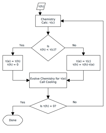
Figure 1.— Schematic view of chemistry subcycling. First, the chemical time step, $\tau(c),$ is calculated using eqn. (12). If this is larger than the hydrodynamic time step, then the evolution time step, $\tau(e),$ is set to the hydrodynamic time step. Else, $\tau(e)$ is set to the chemical time step. The network is then evolved for $\tau(e)$ and the remaining time step $\tau(h)$ is calculated. If this is zero then we proceed to the next step, else we cycle back through the network with the updated abundances. This loop continues until the full hydrodynamic time step is covered. Note that after every chemical network iteration, the cooling routine is called.

In cases in which the gas is extremely hot or cold, the chemical make-up can be determined directly from the temperature, avoiding the need for matrix inversions. If the temperature is above $10^{5}$ K then all atomic species become ionized and all molecular species are dissociated, and the network can be bypassed. If the temperature is between $2.0\times 10^{4}$ and $1.0\times 10^{5}$ K , then we ‘prime’ the solutions and ionize 5$\%$ of available neutral hydrogen, 5$\%$ of neutral helium ($4.5\%$ into singly ionized helium and $0.5\%$ into doubly ionized helium), before entering the iterative solver, to help accelerate the routine towards the correct solution. Finally if the temperature is less than 50 K, then all species are kept the same, and no reactions are calculated. This is done because cooling and chemistry rates become unimportant at such low temperatures. It also has the benefit of speeding up the simulation slightly as very little time is spent in either the cooling or chemistry routines. In all other cases, the full network is evolved without alterations.

2.1.2 Chemistry Tests

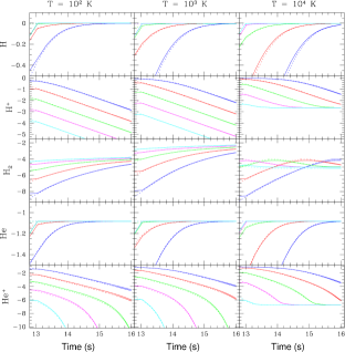
Figure 2.— Chemical evolution tests. Column 1 shows the $T=10^{2}\rm\ K$ case, column 2 shows the $T=10^{3}\rm\ K$ case, and column 3 shows the $T=10^{4}\rm\ K$. Time is given on the $x$-axis and the number density of each species divided by the total number density of hydrogen is given on the $y$-axis. The blue lines correspond to the $n=0.01\ {\rm cm}^{-3}$ case, red to the $n=0.1\ {\rm cm}^{-3}$ case, green to the $n=1.0\ {\rm cm}^{-3}$ case, magenta to the $n=10.0\ {\rm cm}^{-3}$ case, and teal to the $n=100.0\ {\rm cm}^{-3}$ case. The solid lines are results from FLASH and the dashed lines are results from G09.

To test our implemented chemical network, we carried out a series of runs in which initially dissociated and ionized gas was held at constant temperature and density for $10^{16}$ seconds. A small initial time step ($t_{0}\approx$ $10^{6}$ s) was used and allowed to increase up a maximum time step of $10^{12}$ seconds. Models were run with total hydrogen number densities varying from $0.01\ \rm cm^{-3}$ to $100\ \rm cm^{-3}$, and temperatures ranging between $10^{2}\rm\ K$ and $10^{4}\rm\ K$, and no external radiation. In each case, the results were compared to the results of a different implementation of the same chemical network within the ENZO code (Glover 2009, private communication, G09), yielding the molar fractions shown in Figure 2. In this figure, the three columns correspond to runs with different temperatures, the curves corresponds to runs with different densities, and the rows correspond to the evolution of different species.

The match between our tests and the numerical results from G09 is excellent. In all cases and at all temperatures, the curves closely track each other, in most cases leading to curves that are indistinguishable. Although the abundances of several species change by many orders of magnitude throughout the runs, the two methods track each other within to 10% in all cases except for $H_{2}$ at $10^{4}$K, which is unimportant as a coolant but nevertheless consistent within a factor of $1.5$ at all times. Furthermore, this agreement between methods is also seen for deuterium species, which are not shown in this figure as they follow H exactly, maintaining a $\frac{1}{6000}$ ratio between both species at all times.

At $T=100\rm\ K$, all ionized species quickly recombine with the free electrons to form neutral atoms. However, even during this relatively quick transition from ionized to neutral, H⁺ and H^- ions (not shown) persist for long enough to catalyze the formation of substantial amounts of molecular gas, leading to final H₂ molar fractions of $\approx 10^{-4}.$ At $T=1000\rm\ K$, the evolution is very similar to the $T=100\ \rm K$ case, although the species do not reach equilibrium as quickly, leading to even higher levels of H₂ formation. Finally, at $T=10^{4}\rm\ K$, it takes even longer for the ionized hydrogen to recombine, but in this case, less molecular species are formed, as collisional dissociation of H₂ and HD are more prevalent, limiting the maximum amount of these species.

Also apparent in these plot is the dependence of the species evolution on the density of the gas. Chemical reactions are fundamentally collisional processes whose rates are quadratic in number density. Thus, as we are not considering three-body interactions, the timescale associated with chemistry should decrease linearly with the density. This is seen for all temperatures and species shown in Figure 2, as in every case each line is separated from its neighbor by a factor of $10$ in time, exactly corresponding to the density shift between cases.

2.1.3 Effect of the Background Radiation

Background radiation with photon energies between 11.2 and 13.6 eV can excite and dissociate molecular hydrogen. In the absence of other coolants, this can have drastic effect on the evolution of the cloud. Two extremes are immediately apparent, a strong background case in which any H₂ or HD formed is quickly dissociated, and a background-free case in which no molecules are photodissociated. A simple test was constructed to study the effect of the background and determine a fiducial value for $J_{21}$. $J_{21}$ was varied between 0 and 1 at five different values. For each value of $J_{21}$ the number density was varied between $n$ = $10^{-1}$ and $1.0$ cm^-3. Each test was run at a constant temperature and constant density with evolving chemistry and no cooling. The results are given in Figure 3. From this, we determine that only background levels at or above $J_{21}$ = $0.1$ give an appreciable difference in the abundance of H₂ and HD over a megayear timescale, which as we shall see below, is the timescale of shock-minihalo interactions. At the same time, $J_{21}$ = 0.1 provides a reasonable upper limit to the level of background expected before reionization (e.g. Ciardi & Ferrara 2005). Therefore, we use this value as a fiducial value in the simulations with a background.

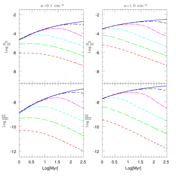
Figure 3.— Comparison of different UV backgrounds. The dotted line is the comparison from G09, the solid line is $J_{21}$ = 0, the short-and-long-dashed line is $J_{21}$ = $10^{-4}$, the dot-long-dahsed line is $J_{21}$ = $10^{-3}$, the dot-short-dashed line is $J_{21}$ = $10^{-2}$, the long-dashed line is $J_{21}$ = $10^{-1}$, and the short-dashed line is $J_{21}$ = 1.0. Time is given on the $x$-axis and number density of each species normalized by the number density of neutral hydrogen is given on the $y$-axis. Note that the solid line and dotted lines coincide with each other, demonstrating that we recover the expected results in the background-free case.

2.2. Cooling

The second major process added to the code was radiative cooling, which was divided into two temperature regimes. At temperatures $\geq 10^{4}$K, cooling results mostly from atomic lines of H and He, with bremmstrahlung radiation also becoming important at temperatures above $10^{7}K$. Below $10^{4}$ K, on the other hand, the net cooling rate is determined by molecular line cooling from H₂ and HD, which, as it is an asymmetric molecule, can radiate much more efficiently than H₂, and thus can be almost as important although it is much less abundant. Cooling from H₂ operates down to $T\leq 200$ K and to number densities $n>10^{4}$ cm^-3 (Glover & Abel 2008; Galli & Palla; 1998), while HD which can cool the gas to slightly lower temperatures and to higher number densities (Bromm, Coppi, & Larson 2002). As we are restricting ourselves to primordial gas in this study at any given temperature the overall cooling rate, $\Lambda_{\rm Total}$, is the combination from both regimes,

$$\Lambda_{\rm Total}=\Lambda_{\rm Atomic}+\Lambda_{\rm Molecular}.$$ (13)

Each cooling rate has the form:

$$\Lambda_{i,j}=n_{i}n_{j}\lambda_{i,j},$$ (14)

where $\Lambda_{i,j}$ is the energy loss per volume due to species i and j, $n_{i}$ and $n_{j}$ are the number densities of each species, and $\lambda_{i,j}$ is the cooling rate in ergs $\rm cm^{-3}\ s^{-1}$. Cooling rates for the collisional excitation between H₂ and H, H₂, H⁺, and e^- and between H${}_{2}^{+}$ and H or e^- are taken from GA08. The cooling rate for the collisional excitation between HD and H is taken from Lipovka, Núñez-López, $\&$ Avila-Reese (2005). Finally, cooling rates from Hydrogen and Helium atomic lines are calculated using CLOUDY (Ferland, G.J., et al 1998). In calculating these rates, we followed the procedure described in Smith et al. (2008) and used the “coronal equilibrium” command which considers only collisional ionization. The cooling curve was calculated assuming case B recombination for the recombination lines of hydrogen and helium, as discussed further in $\S 3.1$.

Any cooling routine contains a natural timescale that relates the total internal energy to the energy loss per time:

$$\tau_{\rm cool}=\frac{\alpha_{\rm cool}\times E_{i}}{\dot{s}},$$ (15)

where $\alpha_{\rm cool}$ is a constant between 0 and 1, in all cases set at 0.1, $E_{i}$ is the internal energy, and $\dot{s}$ is the energy loss per time. Cooling rates are very dependent on temperature and species abundances and these quantities can change rapidly over a single chemical time step.

A method of subcycling over cooling time steps was developed to ensure that the correct cooling rates are used. An initial cooling time scale is calculated assuming $\alpha_{\rm cool}$ = 0.1 using eqn. (15) which is then compared to the chemical time step. If $\tau_{\rm cool}$ is smaller than the fraction of the chemistry time step then that fraction of energy is subtracted from the internal energy and temperature. The cooling rate and cooling time step is recalculated with the updated temperature. This continues until the chemistry time step is reached. This is schematically given in Fig. 4.

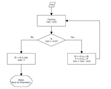
Figure 4.— Schematic view of the cooling subcycle. The time over which chemistry evolves $\tau(e)$ is used as the initial time step. This is compared against $\tau(cl)$ the cooling time step, as given by eq. (15). If the cooling time step is shorter than the evolved time step, then a portion of the internal energy and temperature are subtracted and the evolved time step is updated. The cooling time step is then recalculated. If the cooling time step is longer than the evolving time step then the internal energy is directly updated and used to calculate the new temperature. Once this is done, cooling is complete and we return to the chemistry routine

2.2.1 Cooling Tests

As a test of our cooling routines, we reproduced the example curves given in Prieto et al. (2008). In this work, the authors present the effects of H₂ and HD cooling in a primordial gas. The gas begins at an initial temperature of $T=500$ K with initial number densities, relative to hydrogen: $n_{{\rm H}^{+}}=10^{-4};n_{{\rm H}^{-}}=n_{{\rm H}_{2}^{+}}=10^{-12};n_{{\rm H}_{2}}=10^{-3};n_{\rm D}=10^{-5};n_{{\rm D}^{+}}=10^{-9};n_{{\rm HD}}=10^{-6};n_{{\rm HD}^{+}}=10^{-18};n_{{\rm He}^{+}}=n_{{\rm He}^{++}}=0.0$l and with initial hydrogen and helium densities of $\rho_{\rm H}=0.75\times\rho_{tot}$ and $\rho_{{\rm He}}=0.24\times\rho_{tot}$, where $\rho_{tot}$ is the total baryonic matter density.

Three models were run with total number densities of $n_{tot}=1.0,10.0,$ and $100.0$ cm^-3. Cooling was tracked for $10^{8}\ \rm yrs$ with chemistry evolving simultaneously. The results of this calculation are shown in Figure 5, which indicates good agreement with Prieto et al. (2008). It should be noted that temperature evolution in this plot has a linear dependence of the number density of the gas. For example, a gas with ten times the number densities of another gas will cool ten times quicker. This is again because most of the cooling is coming from the collisions between two species, in this case H₂ or HD and H.

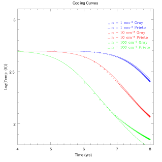
Figure 5.— Cooling tests. The solid lines are taken from Prieto et al. (2008) and compared to our model. The blue curves correspond to a number density $n=1.0\rm\ cm^{-3}$, red to $n=10.0\rm\ cm^{-3}$, and green to $n=100.0\rm\ cm^{-3}$. The temperature is not allowed to go below 50 K.

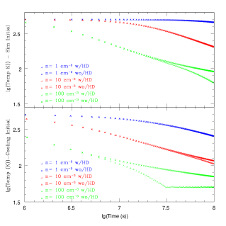
Figure 6.— Test of the impact of HD cooling. The top panel shows the results using primordial abundances while the bottom shows for abundances from the cooling test. Initially, the temperature is started at 500 K and evolved for 100 Myrs.

As mentioned above, HD can be more important than H₂ for gas cooling at higher densities and colder temperatures. To determine whether or not HD cooling is important in this simulation, we apply the cooling test to two different scenarios. First, we use the same initial abundances as described above and second, using primordial abundances with a small fraction ($0.01\%$) of each atomic species ionized. Each test was run twice, once with deuterium and once without. The results of these tests is given in Figure 6. At high number densities, HD cooling does not have a perceivable effect. At intermediate temperatures, HD cooling is important for a gas with the initial abundances from the cooling tests Finally, at low temperatures, HD cooling is very important in both cases.

3. Model Framework

Having developed and tested the chemistry and cooling routines necessary to study minihalo-shock interactions, we next turn to the detailed shock-minihalo interactions. Here we restrict our attention to a Cold Dark Matter (CDM) cosmology, with parameters are $h=0.7$, $\Omega_{0}=0.3$ , $\Omega_{\Lambda}=0.7$, and $\Omega_{b}=0.045$ (e.g. Spergel et al. 2007), where $h$ is the Hubble constant in units of 100 km s^-1 Mpc^-1, $\Omega_{0},\Omega_{\Lambda},$and $\ \Omega_{b}$ are the total matter, vacuum, and baryonic densities, respectively, in units of the critical density. For our choice of $h$, the critical density is $\rho_{crit}=9.2\times 10^{-30}$ g/cm³.

3.1. The Minihalo

A simple model is used for the gas and dark matter of the protocluster whose collapse redshift of $z_{c}=10$ (a cosmic age of $\approx\ 0.5$ Gyr) is taken to be just before the epoch of reionization, and whose total mass of $M_{c}=3.0\times 10^{6}M_{\odot}$ is taken to be on the large end of minihalos formed at this redshift. The gas is assumed to have a primordial composition of 76% neutral atomic hydrogen and 24% neutral atomic helium by mass. Initially, the cluster has a mean density that is enhanced by a factor $\Delta={\rm 178}$ (e.g. Eke, Navarro, & Frenk 1998) above the background, $\rho_{c}=\Delta\Omega_{0}(1+z_{c})^{3}\rho_{\rm crit}=6.54\times 10^{-25}{\rm gm/cm^{3}}$. In this case, the cloud’s virial radius is $R_{c}=0.393\ \rm kpc$ and virial velocity of $v_{c}=6.55\ \rm{km/s}.$ We assume that the radial profile is given by Navarro et al. (1997)

$$\rho(R)=\frac{\Omega_{0}\rho_{c}}{cx(1+cx)^{2}}\frac{c^{2}}{3F(c)}\ \rm gm/cm^{3},$$ (16)

where $c$ is the halo concentration factor, $x$ = $R/R_{c}$ , and $F(t)\equiv\ln(1+t)-\frac{t}{1+t}$. We assume that as the gas collapses inside the dark matter halo, it is shock-heated to its virial temperature, $T_{c}=1650\ \rm K$ and develops a density distribution of isothermal matter in the CDM potential well:

$$\rho_{\rm gas}(R)=\rho_{0}e^{-\left(\frac{v_{\rm esc}^{2}(0)-v_{\rm esc}^{2}(R)}{v_{c}^{2}}\right)}\rm gm/cm^{3}.$$ (17)

where the escape velocity is as a function of radius is given by $v(xR_{\rm vir})=2v_{c}^{2}[F(cx)+cx(1+cx)^{-1}][xF(c)]^{-1}.$ From Madau et al. (2001), we take a typical value of the halo concentration to be $c=4.8,$ although some observations suggest that high-redshift haloes maybe less concentrated than expected from this estimate (Bullock et al. 2001). With this value of $c$, we can compute the central density as:

$$\rho_{0} =\frac{(178/3)c^{3}\Omega_{b}e^{A}\left(1+z\right)^{3}}{\int_{0}^{c}\left(1+t\right)^{A/t}t^{2}dt}\rho_{\rm crit}$$

$$=39215\ \Omega_{b}\rho_{\rm crit}\left(1+z_{c}\right)^{3}$$

$$=2.16\times 10^{-23}{\rm gm/cm^{3}},$$ (18)

where $A\equiv 2c/F(c)=10.3$ and $t=cx$.

To determine which case to use in our chemistry routine the optical depth for H⁺, He⁺, and He⁺⁺ recombination was calculated from this profile:

$$\tau_{\nu}(r)=\int^{r}_{r_{0}}\sigma_{\nu}n(r^{\prime})dr^{\prime},$$ (19)

where $\sigma_{\nu}$ is the cross section of interaction and $n(r^{\prime})$ is the number density. For hydrogen-like atoms the cross section is

$$\sigma_{\nu}=\frac{7.91\times 10^{-18}}{Z^{2}}\left(\frac{\nu_{1}}{\nu}\right)^{3}\ {\rm g}\rm\ \ cm^{2},$$ (20)

where $h\nu_{1}=13.6\ Z^{2}\rm\ eV$ and $Z$ is the nuclear charge. Calculating the optical depth from eqs. (17 - 20) yields the results given in Table 1. We assume for the case of He⁺⁺ recombination, that the surrounding helium is singly ionized. In all cases the optical depth is much greater than 1 (see §3.0) and therefore we use case B rates for all recombination reactions in our fiducial simulations.

Table 1Optical Depths. $\tau$ is the optical depth to the center of the cloud. In all cases the optical depth is much greater than 1.

$\rm Species$	$\rm Incident\ Energy\ eV$	$\rm\ \tau$
$\rm H^{+}$	$13.6$	$3553.9$
$\rm He^{+}$	$24.6$	$1049.2$
$\rm He^{++}$	$54.4$	$280.6$

3.2. Gravity

As the minihalo in our simulation is made up of both gas and collisionless dark matter, a two-part gravity scheme was required. First, the Ricker (2008) multigrid Poisson solver was used to calculate the gravitational potential due to the gas component. Second, the acceleration due to the total matter was calculated using Eq.  (17) above. The general equation for the gravitational acceleration of an ideal gas is given by $a_{\rm Grav}=\frac{k}{\rho(R)m_{p}}\left[T(R)\frac{\partial\rho(R)}{\partial R}+\rho(R)\frac{\partial T(R)}{\partial R}\right]\ \rm cm/s^{2}.$ To account for the dark matter halo’s contribution to gravity, we calculated the gravitational acceleration of the total matter and subtracted its contribution from the baryonic matter in the initial configuration using the above equation with constant temperature. Finally, we added the gravitational contribution from the self-gravity of the gas. The total acceleration is given simply by:

$$a_{\rm Tot}=a_{\rm M,0}-a_{\rm gas,0}+a_{SG},$$ (21)

where $a_{M}$ is the acceleration from the total initial mass density as given by Eq. (17), $a_{\rm gas,0}$ is the contribution from the baryonic matter in the initial configuration, and $a_{SG}$ is the contribution from the self-gravity calculated from the Poisson solver. Initially, when the minihalo gas is in hydrostatic balance with its surroundings, these last two terms will cancel each other and the cloud will remain unchanged. When the cloud is disrupted and cooling takes effect, the self-gravity will cause the cloud to collapse.

The above equations are correct up to the viral radius of the cloud. To ensure a smooth density transition from the cloud, we simply keep the gas outside of the cloud be gravitationally bound to the cloud and solve for the expected density profile. The acceleration here is then,

$$a_{\rm Grav}=-\frac{GM(R>R_{c})}{R^{2}},$$ (22)

and the density is

$$\rho(R>R_{c})=\rho(R_{c})e^{\left({\frac{R_{0}}{R}-\frac{R_{0}}{R_{c}}}\right)},$$ (23)

with $R_{0}$ = $GM_{c}m_{p}$/$k_{b}T$. Here $G$ is the gravitational constant,$m_{p}$ is the mass of a proton, $k_{b}$ is Boltzmann’s constant, and, as above $M_{c}$ and $T_{c}$ are the mass and temperature of the cloud. As $R\rightarrow\infty$, the density goes down to a small fraction of $\rho(R_{c})$. A test of our gravity routine showed that the cloud was able to maintain hydrostatic balance for many dynamical times in the absence of an impinging galaxy outflow.

3.3. The Outflow

A Sedov-Taylor solution is used to estimate the properties of the galactic outflow. The initial input energy is taken to be $E=\epsilon E_{55}({\rm ergs}),$ where $E_{55}$ is the energy of the supernovae driving the wind in units of $10^{55}$ ergs, and the wind efficiency $\epsilon$ is derived from the amount of kinetic energy from the supernovae that is channeled into the outflow. The shock expands into a gas that is $\delta$ times greater than the background at a redshift of $z_{c}$. As in Scannapieco et al. (2004), we assume that the cloud is a distance $R_{s}=3.6\rm\ kpc$, using fiducial values: $z_{c}=10$, $E_{55}=\rm 10$, $M_{6}=3$, $\delta=44$ and $\epsilon=0.3$

With these values, the velocity of the blast front is $v_{s}=415\ \rm km\ s^{-1},$ when it reaches the minihalo, and the resulting temperature of the fully-ionized post-shock medium is $T=2.4\times 10^{6}$ K. By the time the shock has covered the separation distance, $R_{s}$, it will have entrained a mass

$$M_{s,\rm Total}=4.4\times 10^{7}\rm\ M_{\sun},$$ (24)

with a surface density of

$$\sigma_{s}=2.6\times 10^{5}\rm\ M_{\sun}\ kpc^{-2}.$$ (25)

Note that while the above equations are the solutions that come from a simple spherical blast wave, the wind in the simulation is still well-approximated by a plane wave solution, because the size of cloud is much smaller than the distance between the supernova and the cloud.

To model this wind, a time-dependent boundary condition is imposed at the leftmost boundary of the simulation volume. The expected lifetime of the shock is given by $\sigma_{s}=v_{\rm post}\,\rho_{\rm post}\,t_{s},$ where $v_{\rm post}$ is the post-shock velocity of the blast wave, $\rho_{\rm post}$ is the post-shock density, and $\sigma_{s}$ is the surface density of the entrained material. Solving for $t_{s}$ and putting in the appropriate values, the expected shock life time is $t_{s}=2.5\rm\ Myr$. After this time the shock begins to taper off with the density decreasing and temperature increasing and keeping the pressure constant. This is done to prevent the excessive refinement that a sharp cutoff would cause. The density falls off as

$$\frac{\rho(t)}{\rho(0)}=0.01+0.99e^{-\tau_{s}/1.5}$$ (26)

and the temperature rises as

$$\frac{T(0)}{T(t)}=0.01+0.99e^{-\tau_{s}/1.5}\ ,$$ (27)

where $\tau_{s}$ is defined as $\frac{t-1\,\textrm{Myr}}{1\,\textrm{Myr}}$. This also prevents the hydrodynamic (Courant) timestep from becoming extremely short behind the shock, in order to maintain pressure equilibrium in an extremely rarified medium.

Note that in this initial study, the dark matter and gas distributions have been somewhat idealized, and more complicated geometries could be used to model these components in greater detail. For example, a triaxial instead of a spherical distribution could be assumed for the dark matter halo, inhomogeneities could be added to the minihalo gas, and the shock could be assumed to impact the minihalo off-axis. While each of these possibilities would be qualitatively interesting, and naturally alter the final outcome of the halo, they are nevertheless beyond the scope of this study.

4. Results

Our simulations were carried out in a rectangular box with an effective volume of 3.2 $\times 10^{9}$ $\rm pc^{3}$. The $y$-axis and $z$-axis were the same length of 1170 pc and range between [-585, 585] pc while the $x$-axis was twice as long, stretching between [-585, 1170] pc. The shock started on the left boundary while the cloud was centered at [0,0,0] pc. As hydrodynamic refinement criteria, FLASH uses the second derivative of “refinement variables,” normalized by their average gradient over a cell. If this was greater than 0.8, the cell was marked for refinement, and if all the cells in a region lie below 0.2, those cells were marked for derefinement.

A detailed summary of the runs performed is given in Table 2. The runs are labeled as either high or low resolution (H or L), whether atomic H-He recombination follows Case A or Case B (A or B), and whether we impose a UV background (Y or N). The high-resolution, Case B, no-background run (HBN) is taken to as our fiducial run and compared against other choices of parameters below.

Table 2Summary of the numerical simulations in this study.

$\rm Name$	$\rm l_{ref}$	$\rm Resolution(pc)$	$\rm Cooling\ Mode$	$\rm{Background\ (J_{21})}$
$\rm HBN$	$6$	$4.55$	$\rm Case\ B$	$\rm{0}$
$\rm LBN$	$5$	$9.11$	$\rm Case\ B$	$\rm{0}$
$\rm HBY$	$6$	$4.55$	$\rm Case\ B$	$\rm{10^{-1}}$
$\rm LBY$	$5$	$9.11$	$\rm Case\ B$	$\rm{10^{-1}}$
$\rm HAN$	$6$	$4.55$	$\rm Case\ A$	$\rm{0}$
$\rm LAN$	$5$	$9.11$	$\rm Case\ A$	$\rm{0}$

4.1. Hydrodynamic Evolution

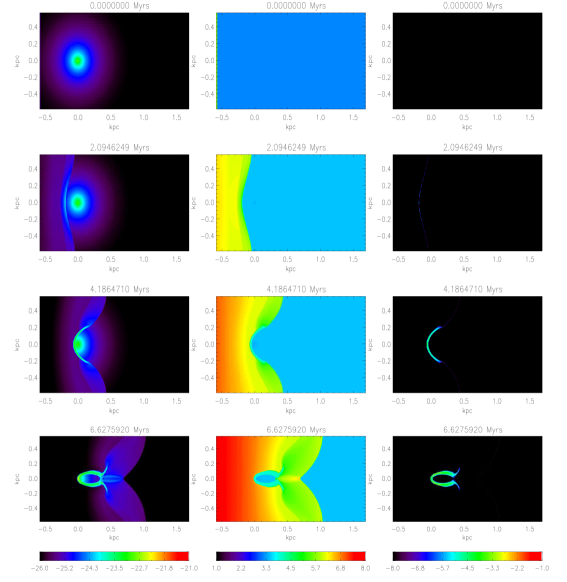
Figure 7.— Initial evolution of the fiducial run, HBN, from $t=0$ through $t=t_{\rm ic}$ the time the shock completely surrounds the cloud. Each row shows the conditions in the central in a slice through the center of the simulation volume at times of 0 (top), 2.1 (second row), 4.2 (third row), and 6.6 Myrs (bottom row). The first column shows contours of the log of density from $\rho_{\rm gas}=10^{-26}$ to 10^-21 g cm^-3, which corresponds to number densities from $n\approx 10^{-2}$ to $10^{2}$, the second column shows contours of the log of temperature from $T=10$ to $10^{8}$K, and the third column shows contours of the log of the H₂ mass fraction from $X_{\rm H_{2}}=10^{-8}$ to $10^{-1}$.

Figure 8.— Final evolution of the cloud from the propagation of the reverse shock across the cloud at $t=7.7$ Myrs (top row), to collapse at $t=11.8$ Myrs (center row), through to the end of the simulation at $t=14.7$ Myrs (bottom row). The panels have been cropped to show only the extended mass along the $x$-axis. Columns, values, and contours are the same as Fig. 7.

In this simulation, several distinct stages of evolution are identified during the interaction between the cloud and the outflow, as shown in Figures  7 and  8. Initially, the cloud is in hydrostatic equilibrium as the shock enters the simulation domain. If it were not supported by pressure, the cloud would collapse on the free-fall time which, using the average cloud density, is

$$t_{\rm ff}=\sqrt{\frac{3\pi}{32G\rho}}\approx 100\rm\ Myr.$$ (28)

As the cloud is initially in hydrostatic balance, the initial sound crossing time is similar to the free-fall time.

As the shock contacts and surrounds the cloud, it heats and begins to ionize the gas. The shock completely envelops the cloud on a characteristic “intercloud” crossing time scale, defined by Klein et al. (1994) as

$$t_{\rm ic}=\frac{2R_{c}}{v_{s}}\approx 4.5\rm\ Myr.$$ (29)

As the cloud is enveloped, the shock moves through the outer regions fastest and ionizes this gas first. This in turn promotes rapid molecule formation as the gas cools and recombines incompletely, leaving H⁺ and H^- to catalyze the formation of H₂ and HD. Interestingly, because the shock slows down as it moves through denser material, the gas behind the center of the halo remains undisturbed until the enveloping shocks meet along the axis at the back of the halo. The leads to a “hollow” H₂ distribution at 6.6 Myrs, in which the molecular coolants are confined to a shell surrounding the undisturbed, purely atomic gas.

After the enveloping shocks collide at the back of the cloud, a strong reflected shock is formed that moves away from the rear of the cloud and back through the halo material. Without cooling, this reflected shock would eventually lead to cloud disruption (Klein et al. 1994). However in our case, the shock has the opposite effect. It moves through the cloud, and the gas is briefly ionized, but then quickly cools and recombines, forming H₂ and HD throughout the cloud. This can be seen in the upper row of Figure 8, which shows the conditions at $\approx 8$ Myrs.

At this point the cloud is denser, smaller, and full of new coolants. Using the conditions from the center of the cloud 8 Myr after the start of the simulation, we calculate new timescales. Now the freefall time is $21$ Myr and the sound crossing time is $\approx 27$ Myr. The cloud is cold and dense enough to start collapsing.

The timescale for the formation of H₂, given in GA08, is

$$t_{\rm H_{2}}=\frac{X_{H_{2}}}{k_{1}X_{e}n}\rm(s),$$ (30)

where $X_{{\rm H}_{2}}$ is the mass fraction of H₂, X_e is the mass fraction of electrons, $k_{1}$ is the reaction rate for the formation of H^- (H + e^- $\rightarrow$ H^- + $\gamma$), and $n$ is the total number density ($\approx$ 1 cm^-3 at 8 Myrs). Initially, as the shock begins to impact the cloud, this timescale is very short, on the order of 0.1 Myrs to get a final abundance of $\approx$ $10^{-5}$. As the abundance of H₂ increases and the abundance of electrons decrease, this timescale quickly increases. Although as the cloud collapses the density increases which lowers this timescale.

The H₂ cooling timescale, given by Klein et al. (1994) is

$$t_{\rm cool}=\frac{1.5nkT}{n_{{\rm H_{2}}}n_{{\rm H}}\Lambda_{{\rm H,H_{2}}}}\rm\ (s),$$ (31)

where $n_{{\rm H}_{2}}$ and $n_{H}$ are the number densities of H₂ and H respectively, and $\Lambda_{{\rm H,H_{2}}}$ is the cooling rate between H and H₂. At 8 Myr the H₂ cooling time in most of the cloud is only $0.2$ Myr, meaning that pressure support drops dramatically after this time. Any expansion due to shock heating is halted as the gas is quickly cooled by H₂ and HD as they form. Furthermore, as the cloud collapses, the chemistry and cooling timescales decrease, rapidly accelerating the collapse.

The final state of the cloud in our simulation is a thin cylinder stretching from the center of the dark matter halo to several times the initial virial radius. The temperature of this gas is 100 to 200 degrees, much colder than the initial virial temperature. The gas is also much denser than the initial minihalo, reaching values of up to $10^{-21}\ \rm\ cm^{-3}$ or $n\approx 10^{3}$ cm^-3, in the center of the cloud, and even this density is probably only a lower limit set by the resolution of our simulation. On the other hand, the cloud is quite extended along the $x$-axis, with substantial differences in velocity along the cylinder. Thus it is continually stretched and fragments until the end of the simulation at 14.7 Myrs (Row 3 in Figure 8).

Figure 9 shows rendered density contours of the major stages of evolution of the cloud from $t=0$ through the end of the simulation. The first panel shows the initial configuration, with the cloud in hydrostatic equilibrium, and the shock front entering from the left side of the simulation volume. The next panel shows the cloud after being impacted by the shock, highlighting the density enhancement in the outer shell of the minihalo gas. The bottom left panel shows the cloud as it begins to cool and collapse, at a time at which the reverse shock has already passed though the cloud and coolants are found throughout the shocked, recombined material. Finally, the last panel shows the distribution at the end of the simulation. The cloud has now been stretched over a large distance and much of its mass has been accelerated to above the escape velocity, moving outside of the dark matter halo. The dense knots of this material in this figure are tightly gravitationally bound, have number densities approaching $10^{3}$ cm${}^{-3},$ and are destined to form extremely compact stellar clusters.

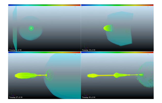
Figure 9.— Rendered density snapshots from the fiducial run, HBN. Colors show contours of log $\rho$ from $10^{-27}$ to $10^{-21}$ cm^-3. The top left panel, $t=$ 0.0 Myrs, shows the initial setup with the stationary minihalo and the shock entering on the left. Top right, $t=$ 6.3 Myrs, shows the state of the cloud as the shock as it envelopes the cloud. Bottom left, $t=$ 9.4 Myrs, shows the cloud during collapse and cooling. Finally, bottom right, $t=$ 14.7 Myrs, shows the final state of the cloud as it is stretched. Dense clumps can be seen in this panel, which we expect to become compact stellar clusters.

4.2. Stellar Clusters

While the collision happens on order of the shock crossing time of the halo, the final distribution of the clumps evolves on the longer timescale defined by $R_{\rm vir}/v_{c}\approx 100$ Myrs. To study the final state of the stretched and collapsed distribution without continuing the simulation out to such extremely long times, we divided the $x$-axis into 100 evenly spaced bins between $x=0$ kpc and $x=1.4$ kpc. We then calculated the mass of each bin by summing up the gas from each cell from the FLASH simulation in a cylinder with a 24 pc radius and length of the bin. Similarly, we calculated the initial velocity of each bin by adding the momentum from each cell within this cylinder and dividing by the total mass in each bin.

We evolved this distribution forward in time using a simple numerical model, which assumed that motions were purely along the $x$ axis and pressure was negligible at late times. In this case, acceleration could be calculated directly from the gravity between each pair of particles and from the potential of the dark matter halo. Furthermore, if any given particle moved past the particle in front of it we merged them together, adding their masses and calculating a new velocity from momentum conservation.

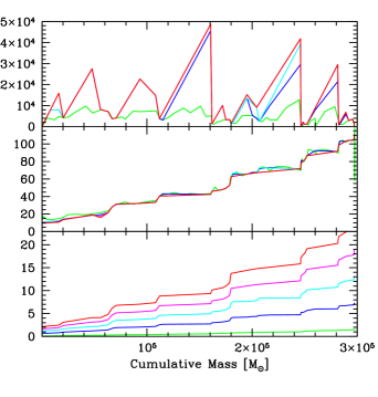
Figure 10.— Evolution of the cloud up to 200 Myrs after the end of the simulation. The $x$-axis in each panel is the cumulative mass in solar masses. The top panel shows the mass of each particle, the middle panel shows their velocities, and the bottom panel shows their positions. The solid green lines show the profile at the end of the simulation $t_{f}=14.7$ Myrs, the dotted blue lines show the profile 50 Myrs later, the short-dashed cyan lines show the profile at $t_{f}+100$ Myrs, the dot-short dashed magenta lines show the profile at $t_{f}+150$ Myrs, and finally the short dash-long dashed red lines show the profile at $t_{f}+200$ Myrs. As time progresses we find that much of the material in the linear feature from Fig. 8 merges together. Most of this merging is complete by 100 Myrs after the end of the simulation.

Evolving the distribution in this way for an additional 200 Myrs past the end of the simulation yielded the results shown in Figure 10. As the stretched cloud continues to move outward, particles begin to attract each other, and eventually merge together to create larger clumps. By 100 Myrs most of the particles have merged, after which their motions are purely ballistic. This can seen in the top panel as the lines for the late times overlap each other and in the middle panel as the velocity profiles overlap.

At the final time of 200 Myrs after the end of numerical simulation, three small, stable clumps with masses of 5.0$\times 10^{4}$ M${}_{\odot},$ 4.0$\times 10^{4}$ M${}_{\odot},$ and $3\times 10^{4}$ $M_{\odot},$ as can be seen in the top panel of Fig. 10. Each of these new peaks is located far outside of the original dark matter halo.

4.3. Case A vs. Case B

At temperatures above $10^{4}$ K, the primary source of cooling is atomic lines from hydrogen and helium. Although we have shown that for the primordial cloud, Case B rates should be used for both the chemical network and cooling functions, Figure 11 shows a comparison between our fiducial run, HBN, and a run in which reaction and cooling rates are taken for case A recombination (HAN). The high temperature Hydrogen-Helium cooling curve is taken from Weirsma et al. (2009). The upper panels show density contours and the bottom show contours of H₂ abundance.

As expected, the Case B simulation produces greater molecular coolant abundance at similar overall densities. This difference can be seen in the lower two panels of the first column of Fig. 11 at 6.63 Myrs. To remain in pressure support as the cloud becomes denser from the shock, the cloud must get hotter. However, because Case A cools slightly faster, this support is quickly removed and the cloud takes on a more extended shape as evident in the first two columns of Fig. 11. Although, by 14 Myrs the abundance of molecular coolants are very similar between HBN and HAN with each containing $X_{H_{2}}\approx 10^{-2.5}$.

In both cases, the fate of the minihalo gas is the same. Atomic cooling occurs sufficiently rapidly to sap the shock of its energy and drop the post-shock temperature to $\approx 10^{4}$ K, and nonequillibrium processes step in to provide molecular coolants below $10^{4}$ K. The gas is then able to collapse and form into a long dense filament within which clumps are formed. In fact the only substantial differences between the runs are the details of the distributions of clumps, which is somewhat more extended in the case A run as compared to the case B run.

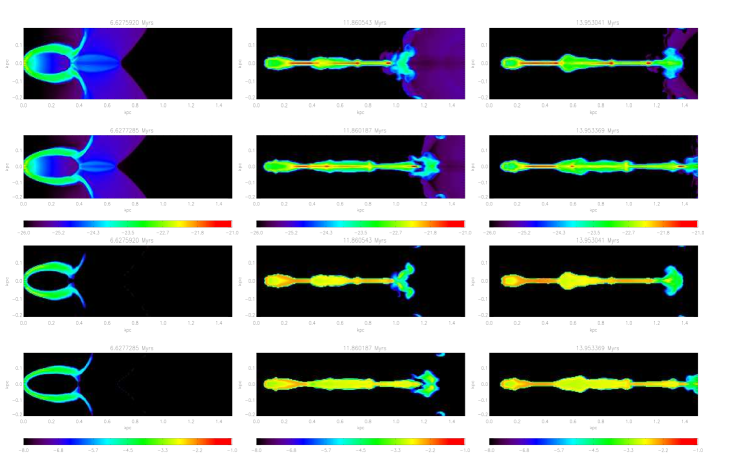
Figure 11.— Comparison between Case A and Case B cooling and chemistry rates. In this plot time varies across columns, moving from $t=6.6$ Myrs (left column), to $7.7$ Myrs (center column), to $14.0$ Myr (right column). The upper two rows show the density in the central slice from the fiducial, case B run (HBN, top row), and the case A run (HAN, second row), with log contours ranging from $\rho=10^{-26}$ to $10^{-21}$ g cm${}^{-3}.$ The lower two rows show the H₂ mass fraction in the fiducial run (third row) and the Case A run (bottom row). Here the log H₂ mass fraction contours range from $X_{\rm H_{2}}=10^{-8}$ to $10^{-1}$.

4.4. UV Background

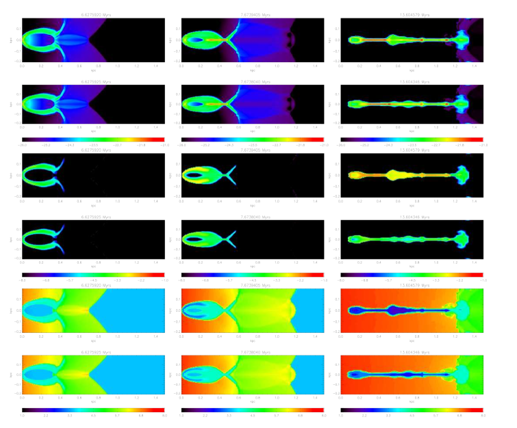
Figure 12.— Comparison between the fiducial run (HBN) and a run including a dissociating background (HBY) at three important stages of evolution. As in Fig.  11, from left to right the columns correspond to $t=6.6,$ 7.7, and 14.0 Myrs. From top to bottom the rows represent log density contours in the fiducial run (Row 1) and the dissociating background run (Row 2), contours of log H₂ mass fraction in run HBN (Row 3) and HBY (Row 4), and contours of log temperature from run HBC (Row 5) and HBY (Row 6). The limits of each panel are the same as Fig 7. The addition of a background greatly reduces H₂ but has almost no effect on the dynamics of the interaction.

A more uncertain aspect of our simulation is our assumption of a negligible dissociating background. In fact, the presence of at least a low level of dissociating background is necessary in order for the minihalo not to collapse and form stars on its own, cooling by H₂ and HD left over from recombination. To set an upper limit on the impact of such a background we modify the rates in our chemical network to approximate a relatively large dissociating background of J${}_{21}=0.1,$ as discussed in section 2.1. Furthermore, as these rates are modified for all reactions throughout the simulation, this background is taken to affect even the densest regions of the cluster. This is equivalent to assuming that the cloud is optically thin to 11.2 to 13.6 eV photons at all times during the simulation.

Figure 12 shows the comparison between the run including this background (HBY) and the fiducial run HBN. As expected, the abundance of H₂ is reduced in the case with the UV background, peaking at about $\approx 10^{-4}$ instead of $\approx 10^{-2}$ in the run without a background. Interestingly, this difference persists even after a few megayears into the simulation, and the abundance of the HPY run remains stable at about $\approx 10^{-4}$.

However, this value is more than sufficient to cool the gas to the same temperature as in HBN. Even with this lower mass fraction, the cooling time is smaller than the dynamical time, and the evolution of the cloud remains essentially unchanged. The cloud collapses and is stretched into the same configuration as found without a background. Dense clouds are again found between 0.2 and 0.4 kpc, at 0.55 kpc, and 0.9 kpc and the density and temperature of each of these clouds is comparable to those found in the fiducial without a background. By neglecting any molecular self-shielding, this represents a worst case scenario for H₂, yet shock minihalo-interactions continue to make compact stellar clusters.

4.5. Resolution

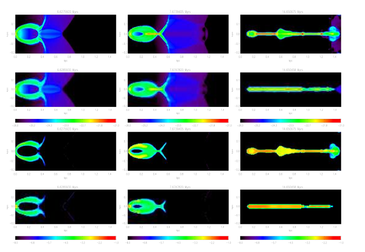
Figure 13.— Impact of maximum levels of refinement. Row 1 and Row 3 show the density and H₂ contours respectively for the fiducial HBN while Row 2 and Row 4 show contours of density and H₂ for LBN. Contour levels are the same as Fig. 11. Time is given at the top of each panel, and proceeds from $t=6.6$ Myrs (left column) to $t=7.7$ Myrs (center column) to $14.7$ Myrs (right column).

Finally, we considered the impact of the maximum refinement level on our results. Figure 13 compares the fiducial run with 6 levels of refinement and an effective resolution of 4.55 pc to a lower resolution run (LBN) with 5 maximum levels of refinement and an effective resolution of 9.1 pc. Here density is shown in the upper two rows in each pair while the mass fraction of H₂ is shown in the bottom two rows.

Only a slight dependence on the formation for H₂ is found with resolution. This is most apparent in the second column, corresponding to $t$ = 7.7 Myrs, which shows that the shocks is slightly broadened in the lower resolution case. Since both chemical reactions and cooling go as $n^{2}$, this smearing out has the effect of slightly decreasing H₂ formation and cooling in the lower resolution run. However, enough H₂ is produced in both cases for the cloud to collapse efficiently, and evolve in the same manner up until late times, when the difference in H₂ abundance is small.

Furthermore, we also conducted similar resolution studies using Case A recombination, and also modifying chemistry and cooling to account for the presence of a dissociating UV background. Again comparisons between the high-resolution runs (HAN and HBY) with the low resolution runs (LAN and LBY) uncovered only weak differences with resolution. Compact stellar clusters were formed in all cases.

4.6. Source of Halo Globular Clusters?

If indeed shock-minihalo interactions lead to massive clusters of stars, the longest-lived stars in these objects will remain observable down to low redshift, providing a direct observational constraint on our results. Furthermore, the clusters formed in our simulations are extremely compact, and thus unlikely to be tidally disrupted as they eventually become gravitationally bound to the ever larger structures that form over cosmological time. As discussed in Scannapieco et al. (2004), the most natural candidate for these old and dense stellar clusters is the population of metal-poor globular clusters, associated with the halos of galaxies (e.g. Zinn 1985; Ashman & Bird 1993; Larsen et al. 2001; Strader et al. 2005; Brodie et al. 2006).

There are several detailed properties of the clusters in our simulations that support this association. Halo globular clusters, like the more metal-rich (disk) globular clusters, are extremely compact, with typical half-light radii of $\approx 3$ pc (e.g. Jordán et al. 2005). Unlike higher-metallicity globular clusters, however, which may have mostly formed at intermediate redshifts (Elmegreen 2010) the age of all metal-poor globular clusters is between $10-13$ Gyrs, placing their formation within or before reionization, during the epoch in which minihalos had not yet been evaporated by ionization fronts.

While globular clusters exits at a range of masses, their mass distribution is well described by a Gaussian in $\log_{10}(M_{gc})$ with a 0.5 dispersion, and mean at $10^{5}$ solar masses, precisely spanning the masses of the clumps formed in our simulations. Although the lower mass limit of globular clusters may be set by destruction through mechanical evaporation (e.g. Spitzer & Thuan 1972) and shocking that occurs as the cluster pass through the host galaxies (e.g. Ostriker et al. 1972), the upper mass limit appears to be an intrinsic property of the initial populations (e.g. Fall & Rees 1985; Peng & Weisheit 1991; Elmegreen 2010). Furthermore, this upper limit of $\approx 10^{6}M_{\odot}$ in stars corresponds roughly with the $10^{4}$ K virial temperature above which atomic cooling becomes effective in high-redshift virialized clouds of gas and dark matter (Fall & Rees 1985). No $\mathrel{\hbox{\hbox to0.0pt{\hbox{\lower 4.0pt\hbox{$\sim$}}\hss}\hbox{$>$}}}10^{6}M_{\odot}$ stellar clusters can result from shock minihalo interactions, because no minihalos exist with gas masses $\mathrel{\hbox{\hbox to0.0pt{\hbox{\lower 4.0pt\hbox{$\sim$}}\hss}\hbox{$>$}}}10^{6}M_{\odot}.$

The second clue as to the origin of globular clusters comes from observations of stars being tidally stripped from these objects. If, like galaxies, globular clusters are contained within individual dark matter halos, the stripping of stars would be highly suppressed, due to the increased gravitational potential. Surprisingly, no such evidence of dark matter halos is seen (Moore 1995), suggesting that these clusters formed through a mechanism markedly different than star formation within galaxies.

Again, the triggered-star formation seen in our shock-minihalo simulations provides a natural explanation of this key observed property. While gas is initially gathered together by a collapsed dark matter potential, the lack of effective coolants prevents this collapse from continuing to the point that stars are formed at the center of the potential. Instead the momentum of the impinging galaxy wind is such that it is able to accelerate the gas above the escape velocity of the halo – even as it induces cooling and compresses the gas to the point that it remains gravitationally bound on its own. The trigger for star formation and the mechanism that removes the dark mater halo are one and the same, resulting in a population of stellar clusters that form at the moment they break free from their dark-matter enclosures.

5. Conclusions

Cosmological minihalos provide the initial building blocks out of which larger dark mater halos and galaxies form. During reionization, these minihalos surrounded all young galaxies and consisted of metal-free neutral atomic gas. The lack of molecules in these objects stalled their evolution at virial temperature below $\approx 10^{4}\rm\ K$ as cooling from atomic hydrogen becomes inefficient and any molecular coolants are dissociated by UV Lyman-Werner photons, too hot for star formation in such small objects. Only interactions that cause non-equilibrium molecule formation could allow the gas in minihalos to collapse and form stars.

Previous work has used ionization fronts to create these conditions (Cen 2001), however, 3D hydrodynamic simulations show that for either a stellar or quasar source, instead of creating clouds of H₂, the cloud is instead completely photo-evaporated (Iliev et al. 2005; Shapiro et al. 2006). However galactic outflows are another option for triggering star formation. Shocks provide the conditions for non-equilibrium chemistry without completely destroying the cloud.

To simulate these interactions, we have added a primordial chemistry network and associated cooling routines into FLASH3.1. This network traces collisional ionization and recombination of hydrogen and helium as well as the formation of two primary coolants in the absence of metals: H₂ and HD. We have also included the impact of a dissociating background on these rates and implemented routines that control the cooling of gas in the presence atomic and molecular line cooling.

With these code developments in place, we have been able to simulate the interaction between a galactic outflow and a primordial minihalo that results in structures that are identified as proto-globular clusters. The shock fills two very important roles. First, it ionizes the neutral gas found in the minihalo, which recombines and begins to form H₂ and HD, through nonequillbrium processes. These coolants allow the cloud to cool to much lower temperatures, triggering star formation. Secondly, the shock imparts momentum into the gas and accelerates it above the escape velocity. This creates a cloud of dense, cold molecular gas that is free from dark matter halos.

Together, these many similarities suggest that there is not only room at low redshifts for the kinds of clusters were see in our simulations, but that low-redshift observations require the formation of stars by a mechanism remarkably similar to the one we are simulating. This physical connection requires further investigation, especially in light of a final remarkable property of globular clusters, the chemical homogeneity of their stars. While there are large metallicity between different globular clusters the dispersion of [Fe/H] within any given cluster is less than 0.1 dex, or a factor of $\approx$ 1.25 (Suntzeff 1993). Usually, this is explained either by pre-enrichment, meaning that stars form out of gas that had already been homogeneously enriched by a previous generation of supernovae (e.g. Elmegreen & Efremov 1997; Bromm & Clarke 2002), or “self-enrichment,” meaning that the protocluster cloud was enriched by one or more SN events occurring within it (e.g., Brown et al. 1995; Cen 2001; Nakasato et al. 2000; Beasley et al. 2003; Li & Burstein 2003). Both types of scenarios have strong flaws. In the pre-enrichment case, the key problem is just exactly what the previous population was, why it played only a secondary role in the formation history of the cluster, and how it could have enriched this material on very short timescales. In the self-enrichment picture, on the other hand, the key problems is that the kinetic energy corresponding to resulting SN is likely to unbind the gaseous protocluster (Peng & Weisheit 1991) long before it enriches the gas. Recent two dimensional numerical simulations of primordial supernova inside minihalos show that they do in fact unbind these systems over a range of supernova types and halo sizes (Whalen et al. 2008b).

Shock minihalo interactions have the potential to combine the best features of both these scenarios, bringing in the metals from an outside source, such that the gas collapses instead of unbinds, but nevertheless explaining how star formation could be synchronized in a large mass of coolant-filled gas. Yet highly homogenous population of stars can only be formed if the incoming, enriched gas and the primordial, minihalo material are sufficiently well mixed before star formation begins. Modeling this process will require simulations that build on the ones here to include metal line cooling above and below $10^{4}$ K and detailed models of subgrid-mixing. Testing this assumption and determining what sets of parameters lead to realistic globular cluster formation will be the focus of the upcoming papers in this series.

References

- (1)
- (2) Abel, T., et al. 2002, Science, 295, 93
- (3) Ahn, K., Shapiro, P.R., Iliev, I.T., Mellema, G., & Pen, U. 2009, ApJ, 695, 1430
- (4) Ashman, K. M., & Bird, C. M. 1993, AJ, 106, 2281
- (5) Bader, G., & Deuflhard, P 1983, Numer. Math. 41, 373
- (6) Barkana R., & Loeb A. 1999, ApJ, 523, 54
- (7) Beasley, M. A., Kawata, D., Pearce, F. R., Forbes, D. A., & Gibson, B. K. 2003, ApJ, 596, L187
- (8) Bond J. R., Szalay A. S., & Silk J. 1988, ApJ, 324, 627
- (9) Brodie, J.P., & Strader, J. 2006, ARA&A, 44, 193
- (10) Bromm, V., Coppi, P.S., & Larson, R. 2002, ApJ, 564, 23
- (11) Bromm, V., & Clarke, C. J. 2002, ApJ, 566, L1
- (12) Brown, J. H., Burkert, A., & Truran, J. W. 1995, ApJ, 440, 666
- (13) Bullock J.S, et al. 2001, MNRAS, 321, 559
- (14) Cen, R. 2001, ApJ, 560, 592
- (15) Ciardi, B., & Ferrara, A. 2005, Space Sci. Rev., 116, 625
- (16) Ciardi, B., Ferrara, A., & Abel, T. 2000, ApJ, 533, 594
- (17) Colella, P., & Glaz, H.M. 1985, JCoPh, 59, 264
- (18) Colella, P., & Woodward P. 1984, JCoPh, 54, 174
- (19) Dalgarno, A., & McCray, R. A. 1972, ARA&A, 10, 375
- (20) Eke, V., Navarro, J., & Frenk, C. 1998, ApJ, 503, 569
- (21) Elmegreen, B. G., 2010, in IAU Symp. 226, Star Clusters Basic Galactic Building Blocks Throughout Time and Space, ed. R. de Grijs & J. Lepine, Cambridge, 3
- (22) Elmegreen, B. G., & Efremov, Y. N. 1997, ApJ, 480, 235
- (23) Fall, S.M., Rees, M.J. 1985, ApJ, 298, 18
- (24) Ferland, G.J., Korista, K.T., Verner, D.A., Ferguson, J.W., Kingdon, J.B., & Verner, E.M. 1998, PASP, 110, 761
- (25) Ferrara, A. 1998, ApJ, 499, L17
- (26) Fragile, C.P., Murray, S.D., & Anninos, P. 2004, ApJ, 604, 74
- (27) Franx, M., Illingworth, G. D., Kelson, D. D., van Dokkum, P. G., & Tran, K.-V. 1997, ApJ, 486, L75
- (28) Fryxell, B., et al. 2000, ApJS, 131, 273
- (29) Fryxell, B., Müller, E., & Arnett. B. 1989, nuas.conf, 100
- (30) Fujita, A., Martin, C. L., Mac Low, M.-M., & Abel, T. 2003, ApJ, 599, 50
- (31) Galli, D., & Palla, F. 1998, AA, 335, 403
- (32) Glover, S.C.O., & Abel, T. 2008, MNRAS, 388, 4 (GA08)
- (33) Glover, S.C.O. 2009, private communication (G09)
- (34) Glover, S.C.O., Savin, D.W. 2009, MNRAS, 393, 991
- (35) Haiman, Z., Able, T., & Madau, P. 2001, ApJ, 551, 599
- (36) Haiman, Z., Rees, M., & Loeb, A. 1997, ApJ, 476, 458 (erratum 484, 985)
- (37) Heckman, T. M., Lehnert, M. D., Strickland, D. K., & Armus, L. 2000, ApJ, 129, 493
- (38) Iliev, I. T., Shapiro, P. R., & Raga, A. C. 2005, MNRAS, 361, 405
- (39) Jordán, A. et al. 2005, ApJ, 634, 1002
- (40) Kang, H., Shapiro, P.R., Fall, M., & Rees, M.J. 1990, ApJ, 363, 488
- (41) Kaps, P., & Rentrop, P. 1979, Numer. Math., 33, 55
- (42) Klamer, I. J., Ekers, R. D., Sadler, E. M., & Hunstead, R. W. 2004, ApJ, 612:L97-L100
- (43) Klein, R., McKee, C.F., & Colella, P. 1994, ApJ, 420, 213
- (44) Larsen, S. S., Brodie, J. P., Huchra, J. P., Forbes, D. A., & Grillmair, C. J. 2001, AJ, 121, 2974
- (45) Lehnert, M. D., & Heckman, T. M. 1996, ApJ, 462, 651
- (46) Li, Y., & Burstein, D. 2003, ApJ, 598, L103
- (47) Lipovka, A., Nunez-Lopez, R., & Avila-Reese, V. 2005, MNRAS, 361, 850
- (48) Mac Low, M., & Shull, J.M. 1986, ApJ, 302, 585
- (49) Madau, P., Ferrara, A., & Rees, M. 2001, ApJ, 555, 92
- (50) Martin, C. L. 1998, ApJ, 506, 222
- (51) Martin, C.L. 1999, ApJ, 513, 156
- (52) Moore, B. 1995, ApJ, 461, L13
- (53) Nakasato, N., Mori, M., & Nomoto, K. 2000, ApJ, 535, 776
- (54) Navarro, J.F., Frenk, C.S, & White, S.D.M. 1997, ApJ, 490, 493
- (55) O’Shea, B.W., & Norman, M.L. 2007, ApJ, 654, 66
- (56) Osterbrock, D.G., Astrophysics of Gaseous Nebulae and Active Galactic Nuclei. University Science Books. 1989.
- (57) Ostriker, J. P., Spitzer, L., & Chevalier, R. A. 1972, ApJ, 176, L51
- (58) Palla, F., Salpeter, E.E., & Stahler, S.W. 1983, ApJ, 271, 632
- (59) Palla, F., & Zinnecker, H. 1988, in IAU Symp. 126, The Harlow Shapley Symposium on Globular Cluster Systems in Galaxies, ed. J. E. Grindlay & A. G. D. Philip (Doredrecht: Reidel), 697
- (60) Peng, W., & Weisheit, J. C. 1991, PASP, 103, 891
- (61) Pettini, M., Kellogg, M., Steidel, C. C., Dickinson, M., Adelberger, K. L., & Giavalisco, M. 1998, ApJ, 508, 539
- (62) Prieto, J. P., Infante, L., & Jimenez, R. 2009, arXiv:0809.276v2
- (63) Ricker, P. M. 2008, ApJS, 176, 293
- (64) Rupke, D. S., Veilleux, S, & Sanders, D. B. 2005, ApJS,160,115
- (65) Sokasian, A., Yoshida, N., Abel, T., Hernquist, L., & Springel, V. 2004, MNRAS. 350, 47
- (66) Scannapieco E., Ferrara A., & Madau P. 2002, ApJ, 574, 590
- (67) Scannapieco, E. et al. 2004. ApJ, 615,29
- (68) Shapiro, P.R., & Kang, H. 1987, ApJ, 318, 32
- (69) Shapiro, P. R., Raga A. C., & Mellema G. 1997, in “Structure and Evolution of the Inter- galactic Medium from QSO Absorption Line Systems,” p. 41
- (70) Shapiro, P. R., Raga A. C., & Mellema G. 1998, Mem. Soc. Astron. Ital., 69, 463
- (71) Shapiro, P. R., Iliev, I. T., & Raga, A. C. 2004, MNRAS, 348, 753
- (72) Shapiro, P. R., Iliev, I. T., Alvarex, M. A., & Scannapieco, E. 2006, ApJ, 648, 992
- (73) Smith, B., Sigurdsson, S., & Abel, A. 2008, MNRAS, 385, 1443
- (74) Spergel, D. N. et al. 2007, ApJ, 170, 377
- (75) Spitzer, L., & Thuan, T. X. 1972, ApJ, 175, 31
- (76) Strader, J., Brodie, J. P., Cenarro, A. J., Beasley, M. A., & Forbes, D. A. 2005, AJ, 130, 1315
- (77) Suntzeff, N., Mateo, M., et al. 1993, ApJ, 481, 208
- (78) Timmes, F.X. 1999, ApJ, 124, 241
- (79) Thacker R. J., Scannapieco E., & Davis M. 2002, ApJ, 202, 581
- (80) Uehara, H. & Inutsuka, Shu-ichiro 2000, ApJ, 531, L91
- (81) Veilleux, S., Cecil, G., & Bland-Hawthorn, J. 2005, ARA&A, 43, 769
- (82) van Breugel, W., Filippenko, A.V., Heckman, T.,Miley, G. 1985, ApJ, 293, 83
- (83) Weirsma, R.., Schaye, J., & Smith, B.D. 2009, MNRAS, 393, 9
- (84) Whalen, D., O’Shea, B.W., Smidt, J., & Norman, M.L. 2008a, ApJ, 679, 925
- (85) Whalen, D., van Veelen, B., O’Shea, B.W., & Norman, M.L. 2008b, ApJ, 682, 49
- (86)
- (87) Wiita, Paul J. 2004, Ap&SS, 293, 235
- (88) Zinn, R. 1985, ApJ, 293, 424
- (89)