Studying springs in series using a single spring

Abstract

Springs are used for a wide range of applications in physics and engineering. Possibly, one of its most common uses is to study the nature of restoring forces in oscillatory systems. While experiments that verify the Hooke’s law using springs are abundant in the physics literature, those that explore the combination of several springs together are very rare. In this paper, an experiment designed to study the static properties of a combination of springs in series using only one single spring is presented. Paint marks placed on the coils of the spring allowed us to divide it into segments, and considered it as a collection of springs connected in series. The validity of Hooke’s law for the system and the relationship between the spring constant of the segments with the spring constant of the entire spring is verified experimentally. The easy setup, accurate results, and educational benefits make this experiment attractive and useful for high school and first-year college students.

1 Introduction

Restoring forces play a very fundamental role in the study of vibrations of mechanical systems. If a system is moved from its equilibrium position, a restoring force will tend to bring the system back toward equilibrium. For decades, if not centuries, springs have been used as the most common example of this type of mechanical system, and have been used extensively to study the nature of restoring forces. In fact, the use of springs to demonstrate the Hooke’s law is an integral part of every elementary physics lab. However, and despite the fact that many papers have been written on this topic, and several experiments designed to verify that the extension of a spring is, in most cases, directly proportional to the force exerted on it [1, 2, 3, 4, 5, 6, 7, 8, 9, 10, 11, 12], not much has been written about experiments concerning springs connected in series. Perhaps one of the most common reasons why little attention has been paid to this topic is the fact that a mathematical description of the physical behaviour of springs in series can be derived easily [13]. Most of the textbooks in fundamental physics rarely discuss the topic of springs in series, and they just leave it as an end of the chapter problem for the student [14, 15].

One question that often arises from spring experiments is, “If a uniform spring is cut into two or three segments, what is the spring constant of each segment?” This paper describes a simple experiment to study the combination of springs in series using only one single spring. The goal is to prove experimentally that Hooke’s law is satisfied not only by each individual spring of the series, but also by the combination of springs as a whole. To make the experiment effective and easy to perform, first we avoid cutting a brand new spring into pieces, which is nothing but a waste of resources and equipment misuse; second, we avoid combining in series several springs with dissimilar characteristics. This actually would not only introduce additional difficulties in the physical analysis of the problem (different mass densities of the springs), but it would also be a source of random error, since the points at which the springs join do not form coils and the segment elongations might not be recorded with accuracy. Moreover, contact forces (friction) at these points might affect the position readings, as well. Instead, we decide just to use one single spring with paint marks placed on the coils that allow us to divide it into different segments, and consider it as a collection of springs connected in series. Then the static Hooke’s exercise is carried out on the spring to observe how each segment elongates under a suspended mass.

In the experiment, two different scenarios are examined: the mass-spring system with an ideal massless spring, and the realistic case of a spring whose mass is comparable to the hanging mass. The graphical representation of force against elongation, used to obtain the spring constant of each individual segment, shows, in excellent agreement with the theoretical predictions, that the inverse of the spring constant of the entire spring equals the addition of the reciprocals of the spring constants of each individual segment. Furthermore, the experimental results allow us to verify that the ratio of the spring constant of a segment to the spring constant of the entire spring equals the ratio of the total number of coils of the spring to the number of coils of the segment.

The experiment discussed in this article has some educational benefits that may make it attractive for a high school or a first-year college laboratory: It is easy to perform by students, makes use of only one spring for the investigation, helps students to develop measuring skills, encourages students to use computational tools to do linear regression and propagation of error analysis, helps to understand how springs work using the relationship between the spring constant and the number of coils, complements the traditional static Hooke’s law experiment with the study of combinations of springs in series, and explores the contribution of the spring mass to the total elongation of the spring.

2 The model

When a spring is stretched, it resists deformation with a force proportional to the amount of elongation. If the elongation is not too large, this can be expressed by the approximate relation $F=-k\,x$, where $F$ is the restoring force, $k$ is the spring constant, and $x$ is the elongation (displacement of the end of the spring from its equilibrium position) [16]. Because most of the springs available today are preloaded, that is, when in the relaxed position, almost all of the adjacent coils of the helix are in contact, application of only a minimum amount of force (weight) is necessary to stretch the spring to a position where all of the coils are separated from each other [17, 18, 19]. At this new position, the spring response is linear, and Hooke’s law is satisfied.

It is not difficult to show that, when two or more springs are combined in series (one after another), the resulting combination has a spring constant less than any of the component springs. In fact, if $p$ ideal springs are connected in sequence, the expression

$$\frac{1}{k}=\sum_{i=1}^{p}\frac{1}{k_{i}}$$ (1)

relates the spring constant $k$ of the combination with the spring constant $k_{i}$ of each individual segment. In general, for a cylindrical spring of spring constant $k$ having $N$ coils, which is divided into smaller segments, having $n_{i}$ coils, the spring constant of each segment can be written as

$$k_{i}=\frac{N}{n_{i}}k\,.$$ (2)

Excluding the effects of the material from which a spring is made, the diameter of the wire and the radius of the coils, this equation expresses the fact that the spring constant $k$ is a parameter that depends on the number of coils $N$ in a spring, but not on the way in which the coils are wound (i.e. tightly or loosely) [13].

In an early paper, Galloni and Kohen [20] showed that, under static conditions, the elongation sustained by a non-null mass spring is equivalent to assuming that the spring is massless and a fraction of one-half of the spring mass should be added to the hanging mass. That is, if a spring of mass $m_{\mathrm{s}}$ and relaxed length $l$ (neither stretched nor compressed) is suspended vertically from one end in the Earth’s gravitational field, the mass per unit length becomes a function of the position, and the spring stretches non-uniformly to a new length $l^{\prime}=l+\Delta l$. When a mass $m$ is hung from the end of the spring, the total elongation $\Delta l$ is found to be

$$\Delta l=\int_{0}^{l}\xi(x)\,\rmd x=\frac{(m+\frac{1}{2}m_{\mathrm{s}})\,g}{k}\,,$$ (3)

where

$$\xi(x)=\frac{m+m_{\mathrm{s}}(l-x)/l}{k\,l}\,g$$ (4)

is the dimensionless elongation factor of the element of length between $x$ and $x+\rmd x$, and $g$ is the acceleration due to gravity. An important number of papers dealing with the static and dynamic effects of the spring mass have been written in the physics education literature. Expressions for the spring elongation as a function of the $n$th coil and the mass per unit length of the spring have also been derived [21, 22, 23, 24, 25, 26, 27, 28, 29, 30, 31, 32, 33, 34, 35, 36].

3 The Experiment

We want to show that, with just one single spring, it is possible to confirm experimentally the validity of equations (1) and (2). This approach differs from Souza’s work [9] in that the constants $k_{i}$ are determined from the same single spring, and there is no need of cutting the spring into pieces; and from the standard experiment in which more than one spring is required.

A soft spring is divided into three separate segments by placing a paint mark at selected points along its surface (see figure 1). These points are chosen by counting a certain number of coils for each individual segment such that the original spring is now composed of three marked springs connected in series, with each segment represented by an index $i$ (with $i=1,2,3$), and consisting of $n_{i}$ coils. An initial mass $m$ is suspended from the spring to stretch it into its linear region, where the equation $F_{i}=-k_{i}\Delta x_{i}$ is satisfied by each segment. Once the spring is brought into this region, the traditional static Hooke’s law experiment is performed for several different suspended masses, ranging from $1.0$ to $50.0\,\mbox{g}$. The initial positions of the marked points $x_{i}$ are then used to measure the relative displacement (elongation) of each segment after they are stretched by the additional masses suspended from the spring (figure 2). The displacements are determined by the equations

$$\Delta x_{i}=(x^{\prime}_{i}-x^{\prime}_{i-1})-l_{i}\,,$$ (5)

where the primed variables $x^{\prime}_{i}$ represent the new positions of the marked points, $l_{i}=x_{i}-x_{i-1}$ are the initial lengths of the spring segments, and $x_{0}=0$, by definition. Representative graphs used to determine the spring constant of each segment are shown in figures 3, 4, and 5.

4 Dealing with the effective mass

As pointed out by some authors [20, 24, 25, 28, 31], it is important to note that there is a difference in the total mass hanging from each segment of the spring. The reason is that each segment supports not only the mass of the segments below it, but also the mass attached to the end of the spring. For example, if a spring of mass $m_{i}$ is divided into three identical segments, and a mass $m$ is suspended from the end of it, the total mass $M_{1}$ hanging from the first segment becomes $m+\frac{2}{3}m_{\mathrm{s}}$. Similarly, for the second and third segments, the total masses turn out to be $M_{2}=m+\frac{1}{3}m_{\mathrm{s}}$ and $M_{3}=m$, respectively. However, in a more realistic scenario, the mass of the spring and its effect on the elongation of the segments must be considered, and equation (3) should be incorporated into the calculations. Therefore, for each individual segment, the elongation should be given by

$$\Delta x_{i}=\frac{(M_{i}+\frac{1}{2}m_{i})\,g}{k_{i}},$$ (6)

where $m_{i}$ is the mass of the $i$th segment, $M_{i}$ is its corresponding total hanging mass, and $k_{i}$ is the segment’s spring constant. Consequently, for the spring divided into three identical segments ($m_{i}=\frac{1}{3}m_{\mathrm{s}}$), the total masses hanging from the first, second and third segments are now $m+\frac{5}{6}m_{\mathrm{s}}$, $m+\frac{1}{2}m_{\mathrm{s}}$ and $m+\frac{1}{6}m_{\mathrm{s}}$, respectively. This can be explained by the following simple consideration: If a mass $m$ is attached to the end of a spring of length $l$ and spring constant $k$, for three identical segments with elongations $\Delta l_{1}$, $\Delta l_{2}$, and $\Delta l_{3}$, the total spring elongation is given by

$$\Delta l =\Delta l_{1}+\Delta l_{2}+\Delta l_{3}$$ (7)

$$=\int_{0}^{\frac{l}{3}}\xi(x)\,\rmd x+\int_{\frac{l}{3}}^{\frac{2l}{3}}\xi(x)\,\rmd x+\int_{\frac{2l}{3}}^{l}\xi(x)\,\rmd x$$

$$=\frac{(m+\frac{5}{6}m_{\mathrm{s}})\,g}{3\,k}+\frac{(m+\frac{1}{2}m_{\mathrm{s}})\,g}{3\,k}+\frac{(m+\frac{1}{6}m_{\mathrm{s}})\,g}{3\,k}$$

$$=\frac{(m+\frac{1}{2}m_{\mathrm{s}})\,g}{k}\,.$$

As expected, equation (7) is in agreement with equation (3), and reveals the contribution of the mass of each individual segment to the total elongation of the spring. It is also observed from this equation that

$$\Delta l_{1}-\Delta l_{2}=\Delta l_{2}-\Delta l_{3}=\frac{(\frac{1}{3}m_{\mathrm{s}})g}{3\,k}=\mbox{const.}$$ (8)

As we know, $\frac{1}{3}m_{\mathrm{s}}$ is the mass of each identical segment, and $k_{1}=k_{2}=k_{3}=3\,k$ is the spring constant for each. Therefore, the spring stretches non-uniformly under its own weight, but uniformly under the external load, as it was also indicated by Sawicky [28].

5 Results and Discussion

Two particular cases were studied in this experiment. First, we considered a spring-mass system in which the spring mass was small compared with the hanging mass, and so it was ignored. In the second case, the spring mass was comparable with the hanging mass and included in the calculations.

We started with a configuration of three approximately identical spring segments connected in series; each segment having $12$ coils ($n_{1}=n_{2}=n_{3}=12$)  When the spring was stretched by different weights, the elongation of the segments increased linearly, as expected from Hooke’s law. Within the experimental error, each segment experienced the same displacement, as predicted by (8). An example of experimental data obtained is shown in table Tables and table captions.

Simple linear regression was used to determine the slope of each trend line fitting the data points of the force versus displacement graphs. Figure 3(a) clearly shows the linear response of the first segment of the spring, with a resulting spring constant of $k_{1}=10.3\,\pm\,0.1\,\mbox{N/m}$. A similar behaviour was observed for the second and third segments, with spring constants $k_{2}=10.1\,\pm\,0.1\,\mbox{N/m}$, and $k_{3}=10.2\,\pm\,0.1\,\mbox{N/m}$, respectively. For the entire spring, the spring constant was $k=3.40\pm\,0.01\,\mbox{N/m}$, as shown in figure 3(b). The uncertainties in the spring constants were calculated using the correlation coefficient $R$ of the linear regressions, as explained in Higbie’s paper “Uncertainty in the linear regression slope” [37]. Comparing the spring constant of each segment with that for the total spring, we obtained that $k_{1}=3.03\,k$, $k_{2}=2.97\,k$ and $k_{3}=3.00\,k$. As predicted by (2), each segment had a spring constant three times larger than the resulting combination of the segments in series, that is, $k_{i}=3\,k$.

The reason why the uncertainty in the spring constant of the entire spring is smaller than the corresponding spring constants of the segments may be explained by the fact that the displacements of the spring as a whole have smaller “relative errors” than those of the individual segments. Table Tables and table captions shows that, whereas the displacements of the individual segments $\Delta x_{i}$ are in the same order of magnitude that the uncertainty in the measurement of the elongation ($\pm 0.002\,\mbox{m}$), the displacements of the whole spring $\Delta x_{\mathrm{s}}$ are much bigger compared with this uncertainty.

We next considered a configuration of two spring segments connected in series with $12$ and $24$ coils, respectively ($n_{1}=12$, $n_{2}=24$). Figure 4(a) shows a graph of force against elongation for the second segment of the spring. We obtained $k_{2}=5.07\,\pm\,0.03\,\mbox{N/m}$ using linear regression. For the first segment and the entire spring, the spring constants were $k_{1}=10.3\,\pm\,0.1\,\mbox{N/m}$ and $k=3.40\,\pm\,0.01\,\mbox{N/m}$, respectively, as shown in figure 4(b). Then, we certainly observed that $k_{1}=3.03\,k$ and $k_{2}=1.49\,k$. Once again, these experimental results proved equation (2) correct ($k_{1}=3\,k$ and $k_{2}=\frac{3}{2}\,k$).

We finally considered the same two spring configuration as above, but unlike the previous trial, this time the spring mass ($4.5\pm 0.1\,\mbox{g}$) was included in the experimental calculations. Figures 5(a)–(b) show results for the two spring segments, including spring masses, connected in series ($n_{1}=12$, $n_{2}=24$). Using this method, the spring constant for the whole spring was found to be slightly different from that obtained when the spring was assumed ideal (massless). This difference may be explained by the corrections made to the total mass as given by (7). The spring constants obtained for the segments were $k_{1}=2.94\,k$ and $k_{2}=1.51\,k$ with $k=3.34\pm 0.04\,\mbox{N/m}$ for the entire spring. These experimental results were also consistent with equation (2). The experimental data obtained is shown in table Tables and table captions.

When the experiment was performed by the students, measuring the positions of the paint marks on the spring when it was stretched, perhaps represented the most difficult part of the activity. Every time that an extra weight was added to the end of the spring, the starting point of each individual segment changed its position. For the students, keeping track of these new positions was a laborious task. Most of the experimental systematic error came from this portion of the activity. To obtain the elongation of the segments, using equation (5) substantially facilitated the calculation and tabulation of the data for its posterior analysis. The use of computational tools (spreadsheets) to do the linear regression, also considerably simplified the calculations.

6 Conclusions

In this work, we studied experimentally the validity of the static Hooke’s law for a system of springs connected in series using a simple single-spring scheme to represent the combination of springs. We also verified experimentally the fact that the reciprocal of the spring constant of the entire spring equals the addition of the reciprocal of the spring constant of each segment by including well-known corrections (due to the finite mass of the spring) to the total hanging mass. Our results quantitatively show the validity of Hooke’s law for combinations of springs in series [equation (1)], as well as the dependence of the spring constant on the number of coils in a spring [equation (2)]. The experimental results were in excellent agreement, within the standard error, with those predicted by theory.

The experiment is designed to provide several educational benefits to the students, like helping to develop measuring skills, encouraging the use of computational tools to perform linear regression and error propagation analysis, and stimulating the creativity and logical thinking by exploring Hooke’s law in a combined system of springs in series simulated by a single spring. Because of it easy setup, this experiment is easy to adopt in any high school or undergraduate physics laboratory, and can be extended to any number of segments within the same spring such that all segments represent a combination of springs in series.

References

Tables and table captions

Table 1: Spring divided into three identical segments ($n_{1}=n_{2}=n_{3}=12$). The $\Delta x_{i}$ corresponds to the relative displacement of the $i$th segment (with $i=1,2,3$), and $\Delta x_{\mathrm{s}}$ represents the relative displacement of the entire spring.

Displacement					Force
($\pm\,0.002\,\mbox{m}$)					$(\pm\,0.001\,\mbox{N}$)
$\Delta x_{1}$	$\Delta x_{2}$	$\Delta x_{3}$	$\Delta x_{\mathrm{s}}$		$F$
0.000	0.000	0.000	0.000		0.000
0.005	0.005	0.005	0.015		0.049
0.010	0.010	0.010	0.030		0.098
0.015	0.014	0.015	0.044		0.147
0.020	0.019	0.019	0.058		0.196
0.024	0.024	0.025	0.073		0.245
0.029	0.029	0.029	0.087		0.294
0.034	0.034	0.033	0.101		0.343
0.038	0.039	0.039	0.116		0.392
0.043	0.044	0.043	0.130		0.441
0.048	0.048	0.049	0.145		0.491

Table 2: Spring divided into non-identical segments ($n_{1}=12$, $n_{2}=24$). The mass of the spring was included in the experimental calculations. The $\Delta x_{i}$ corresponds to the relative displacement of the $i$th segment (with $i=1,2$), and $\Delta x_{\mathrm{s}}$ represents the relative displacement of the entire spring.

Displacement				Force
($\pm\,0.002\,\mbox{m}$)				$(\pm\,0.001\,\mbox{N}$)
$\Delta x_{1}$	$\Delta x_{2}$	$\Delta x_{\mathrm{s}}$		$F$
0.000	0.000	0.000		0.000
0.001	0.003	0.004		0.010
0.002	0.005	0.007		0.020
0.003	0.006	0.009		0.029
0.004	0.008	0.012		0.039
0.005	0.010	0.015		0.049
0.006	0.012	0.018		0.059
0.007	0.014	0.021		0.069
0.008	0.016	0.024		0.078
0.009	0.018	0.027		0.088
0.010	0.020	0.030		0.098

Figure captions

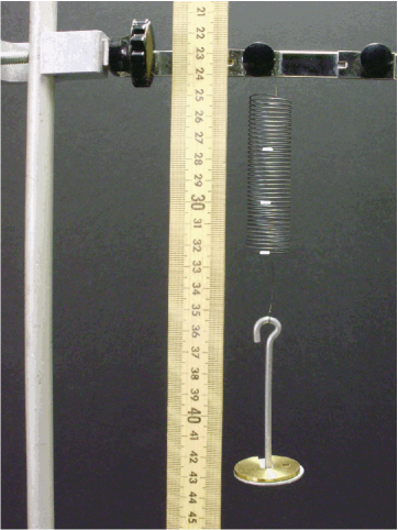
Figure 1: Experimental setup to determine the spring constants of springs in series. A soft spring of mass $m_{\mathrm{s}}=4.43\pm 0.01\,\mbox{g}$, radius $r=1.0\pm 0.1\,\mbox{cm}$, and $n=36$ turns, is divided into segments by using paint marks.

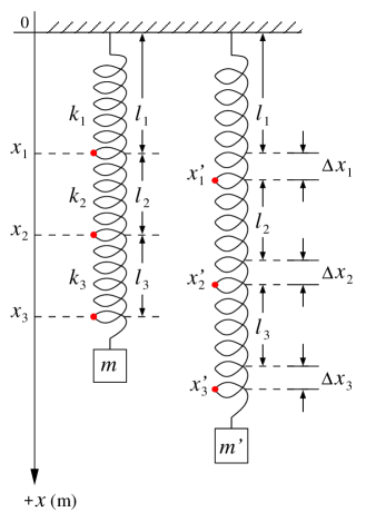
Figure 2: Schematic of the mass-spring system. An initial mass $m$ is suspended from the spring to bring it into its linear region. $l_{i}$ is the initial length of the $i$th spring segment with spring constant $k_{i}$ ($i=1,2,3$). An additional mass $m^{\prime}$ suspended from the spring elongates each segment by a distance $\Delta x_{i}$.

Figure 3: Applied force as a function of the displacement for the first spring segment and the total spring. The spring was considered massless and divided into three identical segments ($n_{1}=n_{2}=n_{3}=12$). (a) The spring constant of the first segment, $k_{1}=10.3\pm 0.1\,\mbox{N/m}$, was obtained from the slope of the trend line. (b) A comparison between elongations of the first segment and total spring. Here, $k=3.40\pm 0.01\,\mbox{N/m}$. The spring constants $k_{2}=10.1\pm 0.1\,\mbox{N/m}$ and $k_{3}=10.2\pm 0.1\,\mbox{N/m}$ were also calculated. It can be observed that $k_{i}=3\,k$, as predicted by equation (2).

Figure 4: Applied force as a function of the displacement for the first and second spring segments, and the total spring. The spring was considered massless and divided into two non-identical segments ($n_{2}=2\,n_{1}=24$). (a) The spring constant of the second segment is $k_{2}=5.07\pm 0.03\,\mbox{N/m}$. (b) A comparison between elongations of the first and second segments with the total spring. $k_{1}=10.3\pm 0.1\,\mbox{N/m}$ and $k=3.40\pm 0.01\,\mbox{N/m}$. Here, $k_{1}=3\,k$ and $k_{2}=\frac{3}{2}\,k$.

Figure 5: Applied force as a function of the displacement for the first and second spring segments, and the total spring. The mass of the spring was included in the experimental calculations, and the spring divided into two non-identical segments ($n_{2}=2n_{1}=24$). (a) The spring constants of the segments were calculated with the corrections to the mass. The second segment has a spring constant of $k_{2}=5.05\pm 0.09\,\mbox{N/m}$. (b) Differences between the spring elongations of the two segments and the total spring are shown. Here, $k=3.34\pm 0.04\,\mbox{N/m}$.

References

- [1] Mills D S 1981 The spring and mass pendulum: An exercise in mathematical modeling Phys. Teach. 19 404–5
- [2] Cushing J T 1984 The spring-mass system revisited Am. J. Phys. 52 925–33
- [3] Easton D 1987 Hooke’s law and deformation Phys. Teach. 25 494–95
- [4] Hmurcik L, Slacik A, Miller H and Samoncik S 1989 Linear regression analysis in a first physics lab Am. J. Phys. 57 135–38
- [5] Sherfinski J 1989 The nonlinear spring and energy conservation Phys. Teach. 27 552–53
- [6] Glaser J 1991 A Jolly project for teaching Hooke’s law Phys. Teach. 29 164–65
- [7] Menz P G 1993 The physics of bungee jumping Phys. Teach. 31 483–87
- [8] Wagner G 1995 Apparatus for teaching physics: Linearizing a nonlinear spring Phys. Teach. 33 566–67
- [9] Souza F M, Venceslau G M and Reis E D 2002 A new Hooke’s law experiment Phys. Teach. 40 35–36
- [10] Struganova I 2005 A spring, Hooke’s law, and Archimedes’ principle Phys. Teach. 43 516–18
- [11] Freeman W L and Freda R F 2007 A simple experiment for determining the elastic constant of a fine wire Phys. Teach. 45 224–27
- [12] Euler M 2008 Hooke’s law and material science projects: Exploring energy and entropy springs Phys. Educ. 43 57–61
- [13] Gilbert B 1983 Springs: Distorted and combined Phys. Teach. 21 430–34
- [14] Giancoli D C 2000 Physics for Scientist and Engineers, 3th ed. (Upper Saddle River: Prentice Hall) p 382
- [15] Serway R A and Jewett Jr J W 2010 Physics for Scientist and Engineers, 8th ed. (Belmont: Brooks/Cole) p 462
- [16] Symon K R 1971 Mechanics (Reading: Addison-Wesley) p 41
- [17] Glanz P K 1979 Note on energy changes in a spring Am. J. Phys. 47 1091–92
- [18] Prior R M 1980 A nonlinear spring Phys. Teach. 18 601
- [19] Froehle P 1999 Reminder about hooke’s law and metal springs Phys. Teach. 37 368
- [20] Galloni E E and Kohen M 1979 Influence of the mass of the spring on its static and dynamic effects Am. J. Phys. 47 1076–78
- [21] Edwards T W and Hultsch R A 1972 Mass distribution and frequencies of a vertical spring Am. J. Phys. 40 445–49
- [22] Heard T C and Newby Jr N D 1977 Behavior of a soft spring Am. J. Phys. 45 1102–6
- [23] Lancaster G 1983 Measurements of some properties of non-Hookean springs Phys. Educ. 18 217–20
- [24] Mak S Y 1987 The static effectiveness mass of a Slinky™Am. J. Phys. 55 994–97
- [25] French A P 1994 The suspended Slinky—A problem in static equilibrium Phys. Teach. 32 244–45
- [26] Hosken J W 1994 A Slinky error Phys. Teach. 32 327
- [27] Ruby L 2000 Equivalent mass of a coil spring Phys. Teach. 38 140–41
- [28] Sawicki M 2002 Static elongation of a suspended Slinky™Phys. Teach. 40 276–78
- [29] Ruby L 2002 Slinky models Phys. Teach. 40 324
- [30] Toepker T P 2004 Center of mass of a suspended Slinky: An experiment Phys. Teach. 42 16–17
- [31] Newburgh R and Andes G M 1995 Galileo Redux or, how do nonrigid, extended bodies fall? Phys. Teach. 33 586–88
- [32] Bowen J M 1982 Slinky oscillations and the notion of effective mass Am. J. Phys. 50 1145–48
- [33] Christensen J 2004 An improved calculation of the mass for the resonant spring pendulum Am. J. Phys. 72 818–28
- [34] Rodríguez E E and Gesnouin G A 2007 Effective mass of an oscillating spring Phys. Teach. 45 100–3
- [35] Gluck P 2010 A project on soft springs and the slinky Phys. Educ. 45 178–85
- [36] Essén H and Nordmark A 2010 Static deformation of a heavy spring due to gravity and centrifugal force Eur. J. Phys. 31 603–9
- [37] Higbie J 1991 Uncertainty in the linear regression slope Am. J. Phys. 59 184–85