Dynamics of Solids in the Midplane of Protoplanetary Disks: Implications for Planetesimal Formation

Abstract

We present local two-dimensional (2D) and three-dimensional (3D) hybrid numerical simulations of particles and gas in the midplane of protoplanetary disks (PPDs) using the Athena code. The particles are coupled to gas aerodynamically, with particle-to-gas feedback included. Magnetorotational turbulence is ignored as an approximation for the dead zone of PPDs, and we ignore particle self-gravity to study the precursor of planetesimal formation. Our simulations include a wide size distribution of particles, ranging from strongly coupled particles with dimensionless stopping time $\tau_{s}\equiv\Omega t_{\rm stop}=10^{-4}$ to marginally coupled ones with $\tau_{s}=1$ (where $\Omega$ is the orbital frequency, $t_{\rm stop}$ is the particle friction time), and a wide range of solid abundances. Our main results are: 1. Particles with $\tau_{s}\gtrsim 10^{-2}$ actively participate in the streaming instability, generate turbulence and maintain the height of the particle layer before Kelvin-Helmholtz instability is triggered. 2. Strong particle clumping as a consequence of the streaming instability occurs when a substantial fraction of the solids are large ($\tau_{s}\gtrsim 10^{-2}$) and when height-integrated solid to gas mass ratio $Z$ is super-solar. We construct a toy model to offer an explanation. 3. The radial drift velocity is reduced relative to the conventional Nakagawa-Sekiya-Hayashi (NSH) model, especially at high $Z$. Small particles may drift outward. We derive a generalized NSH equilibrium solution for multiple particle species which fits our results very well. 4. Collision velocity between particles with $\tau_{s}\gtrsim 10^{-2}$ is dominated by differential radial drift, and is strongly reduced at larger Z. This is also captured by the multi-species NSH solution. Various implications for planetesimal formation are discussed. In particular, we show there exist two positive feedback loops with respect to the enrichment of local disk solid abundance and grain growth. All these effects promote planetesimal formation.

1. Introduction

Planets are believed to be formed out of dust grains that collide and accrete into larger and larger bodies in the gaseous protoplanetary disks (PPDs) (Safronov, 1969; Chiang & Youdin, 2009). The remarkable growth of dust into planets covers 40 orders of magnitude in mass, and can be divided into three regimes. At centimeter size or less, chemical bond and electrostatic forces allow small dust grains to stick to each other to form larger aggregates (Dominik & Tielens, 1997; Blum & Wurm, 2000, 2008). At kilometer or larger sizes (i.e., planetesimals and larger bodies), gravity is strong enough to retain collision fragments, leading to the formation of planetary embryos/cores (Wetherill & Stewart, 1989; Lissauer & Stewart, 1993; Kokubo & Ida, 1998; Goldreich et al., 2004), and ultimately to terrestrial and giant planets (Pollack et al., 1996; Ida & Lin, 2004a, b; Kenyon & Bromley, 2006). The intermediate size range lies in the regime of planetesimal formation. This is probably the least understood process in planet formation, largely because of solid growth in this regime is subject to a bottleneck known as the “meter size barrier”.

In the intermediate size range, aerodynamic coupling between gas and solids is important. The gaseous disk is partially supported by a radial pressure gradient, and rotates at sub-Keplerian velocity, while solid bodies tend to orbit at Keplerian velocity. Consequently, solid bodies feel a headwind and drift radially inwards due to gas drag. The infall time scale is of the order $10^{2}$ years for meter-sized bodies (Weidenschilling, 1977), which poses strong constraint on the timescale of planetesimal formation. Moreover, the collision velocity between meter sized boulders and other bodies is large enough to result in bouncing or fragmentation (Güttler et al., 2009; Zsom et al., 2010), rather than growth. To overcome the meter size barrier, collective effects that form planetesimals out of meter sized or smaller bodies appear to be essential. For example, Cuzzi et al. (2001) proposed the turbulent concentration of chondrule sized particulates by factors of up to $10^{5}$ by extrapolating experimental results to high Reynolds numbers. It such dense regions, mutual gravity of the particulates as a whole can overcome ram pressure and draw them together to form planetesimals (Cuzzi et al., 2008), although the intermittency in the turbulence might work against particle concentration (Youdin & Shu, 2002).

One favorable model of planetesimal formation involves gravitational instability (GI) in the settled dust layer in the midplane of PPDs (Safronov, 1969; Goldreich & Ward, 1973). In the absence of turbulence in the disk, the dust layer would become thinner and thinner until GI sets in and leads to formation of planetesimals by gravitational collapse and fragmentation. However, as first pointed out by Weidenschilling (1980), turbulence generated by vertical shear across the midplane dust layer (via the Kelvin-Helmholtz instability, hereafter KHI) prevents dust grains from continuously settling well before GI is able to operate. Based on the classical criterion for the onset of the KHI and solar metalicity for height-integrated dust to gas mass ratio (hereafter, solid abundance, denoted by Z), the maximum solid density in disk midplane was found to be generally 1-2 orders of magnitude lower than the Roche density for the onset of GI (Sekiya, 1998; Youdin & Shu, 2002) . Inclusion of Coriolis force (Gómez & Ostriker, 2005) as well as radial shear (Chiang, 2008; Barranco, 2009) do not alter the conclusion qualitatively. It appears that increasing the local solid abundance by a factor of 2-10 times solar is needed for this mechanism to operate. This factor may be achievable by photoevaporation of gas (Throop & Bally, 2005; Alexander & Armitage, 2007), and by the radial variations of orbital drift speeds induced by gas drag (Youdin & Shu, 2002; Youdin & Chiang, 2004).

An important ingredient of particle-gas interaction in the midplane solid layer is the backreaction from particles to the gas. The momentum feedback from solids to gas is responsible for KHI which tends to maintain a finite thickness of the solid layer. When the solids are not too strongly coupled to the gas, the backreaction leads to a powerful drag instability (Goodman & Pindor, 2000), now termed the “streaming instability” (hereafter SI, Youdin & Goodman, 2005). The most remarkable feature of the SI is that it very efficiently concentrates particles into dense clumps (Youdin & Johansen, 2007; Johansen & Youdin, 2007), and enhances local particle density by a factor of up to $10^{3}$. Such enhancement in particle density is sufficient to trigger GI, and Johansen et al. (2007, 2009) found in their simulations that planetesimals form rapidly once self-gravity is turned on. The sizes of the planetesimals formed in the simulations are about a few hundreds kilometers, consistent with constraints deduced from observations of asteroid and Kuiper belt objects that planetesimals are formed big (Morbidelli et al., 2009). These results provide a very promising path for forming planetesimals by SI followed by gravitational collapse.

Planetesimal formation is also affected by external turbulence in PPDs. The typical mass accretion rate of $10^{-8\pm 1}M_{\bigodot}\$yr^-1 for T-Tauri stars (Hartmann et al., 1998) indicates efficient angular momentum transport in PPDs. Magnetic field seems certain to play a crucial role in the transport process, most noticeably by the magnetorotational instability (MRI) (Balbus & Hawley, 1991; Hawley & Balbus, 1991). The turbulence generated by MRI strongly affect the settling of small dust grains (Fromang & Nelson, 2009; Balsara et al., 2009; Tilley et al., 2009), but more interestingly, it promotes the concentration of decimeter to meter sized bodies (Fromang & Nelson, 2005; Johansen et al., 2006b, 2007). PPDs are, however, only weakly ionized. The main ionization sources such as cosmic rays and X-rays from the protostar only ionize the surface of the disk, making the surface layers “active” to MRI driven turbulence, while the midplane remains poorly ionized and “dead” (Gammie, 1996). Accretion is therefore layered and mainly proceeds in the active zone. Moreover, the presence of small dust grains substantially increases disk resistivity and reduces the extent of the active layer (Sano et al., 2000; Ilgner & Nelson, 2006; Salmeron & Wardle, 2008; Bai & Goodman, 2009). These non-ideal MHD effects due to partial ionization and dust resistivity, as well as the layered accretion structure in PPDs tremendously complicate the story of planetesimal formation.

In this paper, we consider a local patch of PPDs and study the dynamics of gas and solids in the disk midplane. We perform shearing box hybrid simulations with both gas and particles using the Athena code (Stone et al., 2008). The implementation of the particle module and code tests are presented in Bai & Stone (2010a). The inclusion of backreaction from particles to gas allows us to investigate both the SI and KHI simultaneously. The local model is necessary for studying SI because the scale of particle clumping is much smaller than gas scale height and requires at least $16$ cells to be properly resolved (Bai & Stone, 2010a). The self-gravity from particles is neglected. Although self-gravity will ultimately play an important role in planetesimal formation, our focus is its precursor: clumping of particles. Neglecting self-gravity also has the advantage that our results can be easily scaled to different disk parameters and have very broad applications (see §2.2). We have also neglected the thermodynamics in our work, which may affect the buoyancy of the gas, but the dynamics of the particles are generally unaffected (Garaud & Lin, 2004).

Our ultimate goal is to build the most realistic local model of PPDs possible, including all of the non-ideal MHD effects as well as dust grains/solid bodies in a self-consistent manner. In this paper, however, we focus on the dynamics in the dead zone, and therefore can neglect MHD. This simplification is justified in two ways. First, conductivity calculations have shown that the inner part of PPDs ($r\lesssim 10$AU) almost always contains a dead zone (Bai & Goodman, 2009; Turner & Drake, 2009). Second, this approach separates the hydrodynamic effects (SI) from non-ideal magnetohydrodynamic (MHD) effects, which sets the foundation for more sophisticated work. In reality, the dynamics in the dead zone can be affected by the turbulence in the active layer (Fleming & Stone, 2003). For example, the gas motion in the disk midplane may exhibit strong low-frequency (compared with orbital frequency $\Omega$) vertical oscillations excited by the turbulence in the upper layer, and no coherent anti-cyclic vortices are found (Oishi & Mac Low, 2009). Its influence to the dynamics of the solids is not clear and is left for future investigations.

An important ingredient of our simulations is the size distribution of particles. A wide size distribution of dust grains from micron to millimeter or centimeter size in the PPDs is routinely deduced from the modeling of their spectral energy distribution (SED) (Chiang et al., 2001; Testi et al., 2003; D’Alessio et al., 2006). Theoretical modeling of dust coagulation also result in a broad range of particle sizes (Dullemond & Dominik, 2005; Brauer et al., 2008a; Birnstiel et al., 2010). In the most recent work that incorporates up-to-date laboratory collision experiment results (Güttler et al., 2009; Zsom et al., 2010), the particle size range that dominates the total solid mass spans about 1-3 magnitude, typically from sub-millimeter to decimeter range. We note that although Johansen et al. (2007, 2009) also considered a size distribution of particles, their particle size is relatively large and the size range is narrow (maximum particle size is 4 times the smallest). In this paper, we choose the particle size range to span 1-3 orders of magnitude, and we assume uniform particle mass distribution in logarithmic size bins. Our choice of the particle size distribution roughly agrees with outcome of coagulation model calculations and serves as a first approximation of reality. We perform a parameter survey on particle size range and height-integrated particle to gas mass ratio (or solid abundance) that cover a substantial fraction of parameter space relevant to planetesimal formation. These simulations self-consistently include the mutual interactions between gas and particles of all sizes (extending the early analytical work by Cuzzi et al., 1993 who assumed all particles are passive), and will help us better understand the environment and precursor of planetesimal formation.

We perform both two-dimensional (2D) and three-dimensional (3D) simulations, where the 2D simulations are axisymmetric (i.e., in the radial-vertical plane). We note that KHI is most prominent in the azimuthal-vertical plane (Johansen et al., 2006a), although fully capturing KHI requires fully 3D simulations including radial shear (Chiang, 2008; Barranco, 2009; Lee et al., 2010a). On the other hand, 2D simulation in the radial-vertical plane is sufficient to capture SI (Youdin & Goodman, 2005; Johansen & Youdin, 2007). While 3D simulations are necessary to capture all possible physical effects in the disk midplane layer, we show in §3.1 that KHI is unlikely to be present in all our 3D simulations, because the turbulence generated by SI is strong enough to prevent the particles from further settling to trigger KHI. Therefore, 2D simulations are also a valid approach to the problem, and are much less time-consuming than the corresponding 3D runs. Moreover, comparison between 2D and 3D simulations can be used for discerning multi-dimension effects, and as a guidance for future studies.

This paper is organized as follows. In §2, we describe our simulation method, model parameters and scaling relations. We also describe the basic properties of the saturated state in all our simulations. We study various aspects of our simulations in the subsequent four sections. In §3 we discuss the vertical structure of the particle layer. In particular, we address the question of what is the dominant process of the midplane dynamics, KHI or SI? We further analyze which particles are actively participating in the instabilities, and which particles behave only passively. In §4 we study the conditions for forming dense clumps from the SI, which preludes planetesimal formation. The composition and dynamics of the dense clumps is also analyzed. §5 deals with the radial transport of particles, including both radial drift and radial diffusion. We study particle collision velocities in §6. We conclude our paper in §7 by summarizing our results and discussing various implications for planetesimal formation. In particular, we summarize the logical connections between various physical effects that may enhance each other and promote planetesimal formation.

2. Method and Simulations

2.1. Formalism

We consider local PPD models and formulate the equations of gas and solids using the shearing sheet approximation (Goldreich & Lynden-Bell, 1965). We choose a local reference frame located at a fiducial radius, corotating at the Keplerian angular velocity $\Omega$. The dynamical equations are written using Cartesian coordinates, with $\hat{\boldsymbol{x}},\hat{\boldsymbol{y}},\hat{\boldsymbol{z}}$ denoting unit vectors pointing to the radial, azimuthal and vertical direction, where ${\boldsymbol{\Omega}}$ is along the $\hat{\boldsymbol{z}}$ direction. The gas density and velocities are denoted by $\rho_{g},{\boldsymbol{u}}$ in this non-inertial frame. We include a distribution of particles coupled with gas via aerodynamic drag, where the velocity of particle $i$ is denoted by ${\boldsymbol{v}}_{i}$. The drag force is characterized by stopping time $t_{\rm stop}$, and equals $({\boldsymbol{u}}-{\boldsymbol{v}})/t_{\rm stop}$ per unit particle mass. Particles with different sizes have different stopping times, labeled by subscript “$k$”. Back reaction from the particles to gas is included, which is necessary for the study of KHI and SI. In this non-inertial frame, the equations for the gas read

$$\frac{\partial\rho_{g}}{\partial t}+\nabla\cdot(\rho_{g}\boldsymbol{u})=0\ ,$$ (1)

$$\begin{split}\frac{\partial\rho_{g}\boldsymbol{u}}{\partial t}&+\nabla\cdot(\rho_{g}\boldsymbol{uu}+P\boldsymbol{I})=\\ \rho_{g}&\bigg{[}2{\boldsymbol{u}}\times{\boldsymbol{\Omega}}+\Omega^{2}x\hat{\boldsymbol{x}}-\Omega^{2}z\hat{\boldsymbol{z}}+\sum_{k}\epsilon_{k}\frac{\overline{\boldsymbol{v}}_{k}-\boldsymbol{u}}{t_{{\rm stop},k}}\bigg{]}\ .\end{split}$$ (2)

where the source terms include Coriolis force, radial tidal potential as well as disk vertical gravity. The last term in the momentum equation represents the backreaction (or momentum feedback) from particles to gas: $\epsilon_{k}$ and $\overline{{\boldsymbol{v}}_{k}}$ denote the local mass density and velocity of particles of type $k$. In this paper we neglect the effect of magnetic fields and focus on the interaction between gas and solids in the dead zone of PPDs (Gammie, 1996). An isothermal equation of state for the gas is used throughout this paper, where $P=\rho_{g}c_{s}^{2}$ and $c_{s}$ is the isothermal sound speed.

Similarly, the equation of motion for particle $i$ of type $k$ can be written as

$$\frac{d\boldsymbol{v}_{i}}{dt}=-2\eta v_{K}\Omega\hat{\boldsymbol{x}}+2{\boldsymbol{v}}_{i}\times{\boldsymbol{\Omega}}+\Omega^{2}x_{i}\hat{\boldsymbol{x}}-\Omega^{2}z_{i}\hat{\boldsymbol{z}}-\frac{\boldsymbol{v}_{i}-\boldsymbol{u}}{t_{{\rm stop},k}}\ .$$ (3)

In the above equation, we have added an inward force term $-2\eta v_{K}\Omega\hat{\boldsymbol{x}}$ to mimic the effect of an outward radial pressure gradient in the gas (Bai & Stone, 2010a), where $\eta v_{K}$ is the difference between gas velocity and the Keplerian velocity in the absence of particles. This term will shift both gas and particle azimuthal velocities by $\eta v_{K}$ relative to those in the real system. To avoid confusion, we always use ${\boldsymbol{u}}$ and ${\boldsymbol{v}}$ to denote velocities that corresponds to the real system (i.e., subtracting the azimuthal velocity component from the simulation by $\eta v_{K}$). Particle self-gravity is ignored as we focus on the dynamics in the midplane of the PPD dead zone and precursor of the planetesimal formation.

In our simulations, we have applied an orbital advection algorithm for both gas and particles (Stone & Gardiner, 2010; Bai & Stone, 2010a), and the actual velocities used in the simulation are measured relative to the linearized Keplerian shear flow: ${\boldsymbol{u}}^{\prime}={\boldsymbol{u}}+(3/2)\Omega x\hat{\boldsymbol{y}}$ for gas flow, and ${\boldsymbol{v}}^{\prime}_{i}={\boldsymbol{v}}_{i}+(3/2)\Omega x\hat{\boldsymbol{y}}$ for individual particles.

2.2. Scaling Relations

Measuring velocities in units of the sound speed, time in units of $\Omega^{-1}$, and length in units of the gas scale height $H_{g}\equiv c_{s}/\Omega$, the parameters in the problem are reduced to the following:

1. The dimensionless particle stopping time $\tau_{k}\equiv\Omega t_{{\rm stop},k}$ for particle species $k$.

2. The solid abundance parameter $Z_{k}$ for each particle species, which measures the height-integrated particle to gas mass ratio.

3. The parameter characterizing the strength of the radial pressure gradient $\Pi\equiv\eta r/H_{g}=\eta v_{K}/c_{s}$.

Below, we apply a disk model and provide the scaling relation between the disk model parameters and these dimensionless parameters used in our simulation.

We adopt a generalized solar nebular model where the disk is vertically isothermal and all the disk quantities have a power law dependence on the radius (Youdin & Shu, 2002)

$$\begin{split}\Sigma_{g}&=1700f_{g}r_{\rm AU}^{-b}{\rm\ g\ cm}^{-2}\ ,\\ T&=280f_{T}r_{\rm AU}^{-c}{\rm\ K}\ ,\\ M_{*}&=f_{M}M_{\bigodot}\ .\end{split}$$ (4)

where $\Sigma_{g}$ is the gas surface mass density, $T$ is the disk temperature, $M_{*}$ is the mass of the central star, and $r_{\rm AU}\equiv r/1$AU. These parameters fix the disk model. Although the global disk profile may not follow the simple power law form, we can always approximate a local patch of the disk in the above form, which is very general. In the standard minimum-mass solar nebular (MMSN) model (Hayashi, 1981), we have $b=3/2,\ c=1/2,\ f_{T}=f_{g}=f_{M}=1$. The radial profiles of other physical quantities are

$$\begin{split}\Omega&=2\pi f_{M}^{1/2}r_{\rm AU}^{-3/2}{\rm\ yr}^{-1}\ ,\\ v_{K}&=30f_{M}^{1/2}r_{\rm AU}^{-1/2}{\rm\ km\ s}^{-1}\ ,\\ c_{s}&=f_{T}^{1/2}r_{\rm AU}^{-c/2}{\rm\ km\ s}^{-1}\ ,\\ H_{g}&=3.4\times 10^{-2}f_{T}^{1/2}f_{M}^{-1/2}r_{\rm AU}^{(3-c)/2}{\rm AU}\ .\end{split}$$ (5)

where in the calculation of the sound speed, we assume the mean molecular weight $\mu=2.33$.

The background gas density profile is

$$\rho_{g,b}(r,z)=\frac{\Sigma_{g}}{\sqrt{2\pi}H_{g}}\exp(-z^{2}/2H_{g}^{2})\ ,$$ (6)

where subscript “$b$” denotes “background”. Using this gas density and sound speed, one can derive the radial pressure gradient in the gaseous disk, thus obtain the amount of reduction $\eta v_{K}$ in the gas rotation velocity. After some algebra, we can derive the pressure length scale parameter

$$\begin{split}\Pi\approx-\frac{1}{2}\frac{d\ln{P}}{d\ln{r}}\frac{c_{s}}{v_{K}}&=\bigg{(}\frac{3+2b+c}{4}-\frac{3-c}{4}\frac{z^{2}}{H_{g}^{2}}\bigg{)}\frac{c_{s}}{v_{K}}\\ &\approx 0.054f_{T}^{1/2}f_{M}^{-1/2}r_{\rm AU}^{1/4}\ .\end{split}$$ (7)

Note that $\Pi=\Pi(r,z)$ depends on both radius and height. Nevertheless, in this paper, our simulation box is concentrated in the disk midplane where $z\ll H_{g}$, therefore we can neglect the dependence of $\Pi$ on $z$. In the last equation of the above formula, we have applied the power law indices of the MMSN model. The dependence on disk temperature $f_{T}$, stellar mass $f_{M}$ as well as disk radius $r$ is relatively weak. It is worth mentioning that the dependence of $\Pi$ on disk mass is only through the surface density profile parameter $b$, free from the scaling parameter $f_{g}$. Therefore, the value $\Pi\approx 0.05$ should apply to a wide range of disk models.

Next we consider the scaling relations for the dimensionless stopping time. Because the gas motion in PPDs is expected to be subsonic, the relevant drag laws from the gas to the solids in PPDs are the Epstein drag law (Epstein, 1924), which applies when particle size is smaller than the gas mean free path, and the Stokes drag law, which applies for larger bodies. We assume all solid bodies have spherical shapes, then the stopping time in these two regimes can be expressed as (Weidenschilling, 1977)

$$t_{\rm stop}=\begin{cases}\dfrac{\rho_{s}a}{\rho_{g}c_{s}}\ ,&\text{$a<9\lambda_{m}/4$ (Epstein regime)},\\ \dfrac{4\rho_{s}a^{2}}{9\rho_{g}c_{s}\lambda_{m}}\ ,&\text{$a>9\lambda_{m}/4$ (Stokes regime)}.\\ \end{cases}$$ (8)

where $\rho_{s}\approx 3$g cm^-3 and $a$ are the density and radius of the solid body, $\lambda_{m}=(n_{g}\sigma)^{-1}=\mu m_{H}/\rho_{g}\sigma$ is the mean free path of the gas, and $\sigma\approx 2\times 10^{-15}$cm² is the molecular collision cross section (Chapman & Cowling, 1970). From the above equations, we see that the particle stopping time depends linearly on gas density in the Epstein regime. Nevertheless, the gas density can be regarded as constant near the disk midplane where we study. Therefore, in our local simulations, we can safely take $t_{\rm stop}$ as depending on particle size $a$ only.

To better handle the relation between particle size and its corresponding stopping time, we express the relation between $\tau_{s}\equiv\Omega t_{\rm stop}$ and $a$ by applying our disk model. The result is

$$\begin{split}\tau_{s}=\max\bigg{[}&4.4\times 10^{-3}a_{\rm cm}f_{g}^{-1}r_{\rm AU}^{b}\ ,\\ &1.4\times 10^{-3}a_{\rm cm}^{2}f_{T}^{-1/2}f_{M}r_{\rm AU}^{(c-3)/2}\bigg{]}\ ,\end{split}$$ (9)

where $a_{\rm cm}$ is the particle radius measure in centimeter. In the MMSN model, at 1 AU, particles smaller than $3$cm are in the Epstein regime. At larger radii, the Epstein regime applies to much larger particles.

2.3. Simulation Setup

Fiducially, we consider the MMSN model at 1 AU, and set the pressure length scale parameter $\Pi=0.05$. This parameter is kept fixed in all our simulations. Instead of considering a particle size distribution in radius, we consider the distribution in $\tau_{s}$. Then one can easily translate it into particle radius given the parameters of the disk model. We discretize a continuous particle size distribution into a number of bins. Each bin covers half a dex in $\tau_{s}$ in the logarithmic scale. For simplicity, we assume a uniform particle mass distribution across the bins, that is, all the particle bins (or particle species) have equal amount of mass. The parameters for the size distribution is therefore the minimum and maximum dimensionless stopping time $\tau_{\rm min}$ and $\tau_{\rm max}$ (translated to $a_{\rm min}$ and $a_{\rm max}$ respectively). Physically, our assumption means that most of the mass of the solids resides in the size range between $a_{\rm min}$ and $a_{\rm max}$ and roughly follows a flat distribution in logarithmic scale. To control the total particle mass, we use the total solid abundance parameter

$$Z=\sum_{k=1}^{N_{\rm type}}Z_{k}\ ,\qquad{\rm with}\ Z_{k}=Z/N_{\rm type}\ ,$$ (10)

where $N_{\rm type}$ is the number of particle types (bins). Currently the best estimate of the solar metallicity is about $0.015$ (Lodders, 2003). A substantial fraction of the metal elements may reside in dust grains and grow into larger bodies. In our simulations, we consider three abundance values $Z=0.01,0.02$ and $0.03$. This choice covers a relatively wide range of disk metallicities. Moreover, because our simulation focuses on a local patch in a PPD, the local abundance may not necessarily be equal to the averaged value in the PPD.

As we explained in §1, we perform simulations in both 2D and 3D. Our 2D simulations are in the $\hat{\boldsymbol{x}}$-$\hat{\boldsymbol{z}}$ plane (i.e. axisymmetric). Details of the implementation and code tests of the particle-gas hybrid scheme are given in Bai & Stone (2010a). Our simulations use the standard shearing box approach (Hawley et al., 1995), where the radial boundary condition is periodic with azimuthal shear. Azimuthal boundary conditions are periodic. Vertical gravity is included in our simulations, and we choose reflection boundary condition in the $\hat{\boldsymbol{z}}$ direction, which is the same as that in Johansen et al. (2009). In general, we use 256 cells in the radial (and azimuthal, if applicable) direction. Guided by Bai & Stone (2010a), properly resolving the SI with $\tau_{s}=0.1$ requires about $128$ cells per pressure length scale $\eta r$. With this required resolution, our simulation box size is typically small, spanning only about $2-4\eta r$. Such small box size is also necessary to capture the typical wavelength of the KHI, if present (Johansen et al., 2006a). In our simulations, we generally use $N_{p}=65536$ particles per type for 2D simulations and $N_{p}=3145728$ particles per type in 3D runs (in which cases $N_{\rm type}=7$). Larger $N_{p}$ are used when $N_{\rm type}$ is smaller to keep the total number of particles similar in all our simulations. Our choice of particle number guarantees at least one particle per cell per particle type around the disk midplane, as required for numerical convergence (Bai & Stone, 2010a).

In our simulations, we set the initial particle density profile to be a Gaussian centered on disk midplane with scale height $H_{d}=0.015H_{g}$ for all particle types. The particle and gas velocities are computed from a multi-species Nakagawa-Sekiya-Hayashi (NSH) equilibrium, where the classical single-species NSH equilibrium (Nakagawa et al., 1986) solution is generalized to include multiple species of particles (see Appendix A). Note that different particles have different velocities, and the velocities of particles and gas depend on $z$.

The choice of our simulation box size and boundary conditions in the vertical direction merit further discussion. In the simulations, gas-particle interaction in the disk midplane generates turbulence and excites vertical motions in the gas. Ideally the vertical box size should extend to a few $H_{g}$, similar to what is used for MRI simulations (e.g., Stone et al., 1996), however, this would make 3D simulations too expensive. We have conducted a series of tests in 2D with a single particle species $\tau_{s}=1$ using different vertical box sizes and either reflecting or periodic boundary conditions. In both cases, particles settle to the disk midplane with a spatial distribution reminiscent of sinusoidal waves that slowly drift in the radial direction. We find that the particle scale height is more intermittent when using periodic boundary conditions. Moreover, periodic boundary conditions appear to suppress asymmetric modes in the gas azimuthal velocity around the disk midplane. Using reflecting boundary conditions, we find essentially no difference between the particle scale heights and clumping properties obtained from different vertical box sizes once the box height is much larger than the particle scale height, although it takes longer for the system to reach a quasi-steady state when a larger vertical box size is used. The drift velocities of the wave-like pattern of particles do differ when different vertical box sizes are used, but they are unlikely to affect the properties discussed in §3 to §6. . Guided by these results, as long as the vertical boundary of our simulation box is well above the scale height of all particle species, one should get converged results from the simulations.

Table 1 lists the parameters of all of our simulations. Our runs are labeled using names with the form R$xy$Z$z$-$n$D, where $x,y$ are integers corresponding to $\tau_{\rm min}=10^{-x}$, and $\tau_{\rm max}=10^{-y}$, $z\equiv 100Z$ represents the solid abundance, and $n=2$ ($n=3$) denotes 2D (3D) simulations. When referring to simulations with fixed $x$ and $y$ but all possible values of $z$ and/or $n$, we omit the Z$z$, and/or the $nD$, parts of the names. We focus on two groups of runs. In the first group, the maximum particle stopping time is $\tau_{\rm max}=0.1$. We use 7 particle species to span three orders of magnitude in stopping time (down to $\tau_{\rm min}=10^{-4}$) for the series of runs labeled R41, while in the series labeled R21, we use three particle species to span one order of magnitude in stopping time (down to $\tau_{\rm min}=10^{-2}$). In the second group of runs, the maximum particle stopping time is $\tau_{\rm max}=1.0$, and the minimum stopping time is chosen to be $\tau_{\rm min}=10^{-3}$ (R30) or $0.1$ (R10). In each series of runs (R41, R21, R30, R10), we perform three 2D simulations with $Z=0.01,0.02$ and $0.03$, and two 3D simulations with $Z=0.01$ and $Z=0.03$. Because of a smaller $\tau_{\rm max}$ in the first group, higher resolution is needed to resolve the SI.

Table 1Run parameters.

Run	$Z/0.01\ ^{1}$	$\tau_{\rm min}$	$\tau_{\rm max}$	$N_{\rm type}\ ^{2}$	$L_{x}\times L_{y}\times L_{z}\ ^{3}$	$N_{x}\times N_{y}\times N_{z}$	$N_{p}\ ^{4}$	$T_{e}\ (T_{s})\ ^{5}$
R41-2D	1,2,3	$10^{-4}$	$10^{-1}$	$7$	$0.1\times-\times 0.2$	$256\times 1\times 512$	$6.6\times 10^{4}$	$1500(1200)$
R41-3D	1,3	$10^{-4}$	$10^{-1}$	$7$	$0.1\times 0.1\times 0.2$	$256\times 256\times 512$	$3.1\times 10^{6}$	$250(200)\ ^{5}$
R21-2D	1,2,3	$10^{-2}$	$10^{-1}$	$3$	$0.1\times-\times 0.2$	$256\times 1\times 512$	$9.8\times 10^{4}$	$900(600)$
R21-3D	1,3	$10^{-2}$	$10^{-1}$	$3$	$0.1\times 0.1\times 0.2$	$256\times 256\times 512$	$6.3\times 10^{6}$	$250(200)\ ^{5}$
R30-2D	1,2,3	$10^{-3}$	$1$	$7$	$0.2\times-\times 0.3$	$256\times 1\times 384$	$6.6\times 10^{4}$	$1200(900)$
R30-3D	1,3	$10^{-3}$	$1$	$7$	$0.2\times 0.2\times 0.3$	$256\times 256\times 384$	$3.1\times 10^{6}$	$450(300)$
R10-2D	1,2,3	$10^{-1}$	$1$	$3$	$0.2\times-\times 0.3$	$256\times 1\times 384$	$9.8\times 10^{4}$	$900(600)$
R10-3D	1,3	$10^{-1}$	$1$	$3$	$0.2\times 0.2\times 0.3$	$256\times 256\times 384$	$6.3\times 10^{6}$	$450(300)\ ^{5}$

¹ Total particle to gas mass ratio, divided by 0.01.

² Number of particle species.

³ Domain size, in unit of gas scale height $H_{g}=c_{s}/\Omega$. Note we have fixed $\Pi=\eta r/H_{g}=0.05$.

⁴ Number of particles per species in the simulation box.

⁵ Total run time in unit of $\Omega^{-1}$. The number in the parenthesis indicates the time of saturation. For R41-3D and R21-3D runs with Z=0.03, we have $T_{e}=280$ and $T_{s}=240$. For run R10-3D, we have $T_{e}=500$ and $T_{s}=450$.

2.4. Simulation Runs and Saturation

To determine when a saturated state is reached in each simulation, we monitor the particle vertical scale height $H_{p,k}$ for each particle species $k$, defined as the rms value of the $z$ coordinate of all particles. Saturation occurs when particle settling and turbulent diffusion are in balance, so that the scale height of all particle species is steady. In Figure 1 we show the time evolution of the vertical scale height for each particle species (marked by different colors) in all our runs. Solid and dashed curves represent 2D and 3D simulations respectively. We see that most of the 2D runs saturate within about 50 orbits. The 3D simulations are very time consuming, so we run them for shorter periods. From Figure 1, all 3D runs saturate before we terminate the simulations, although some just barely so.

In the last column of Table 1, we provide the time of saturation $T_{s}$ (in parentheses) for each simulation. Unless otherwise stated, we will perform data analysis in the time interval between the saturation time $T_{s}$ and the end time of the simulation $T_{e}$. In the R41Z3-2D and R21Z3-2D runs, there are sudden jumps in particle heights followed by settling, and this process repeats over time quasi-periodically. Averaging over many cycles is required to reduce the influence of these intermittent “bursts”. The vertical distribution of the smallest particles in the R41-3D and R21-3D runs with $Z=0.03$ are not fully saturated at the end of our simulations. Nonetheless, the scale heights of the largest particles (which dominate the dynamics) in these runs have reached steady state, therefore we consider them to be saturated.

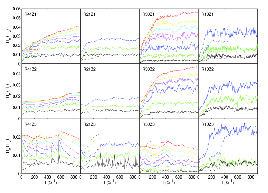
Figure 1.— The time evolution of particle scale height $H_{p}$ for all simulations. Different colors represent different particle species, and particles with smaller $\tau_{s}$ have monotonically larger values of $H_{p}$ (see Table 1 for reference). Results from 2D simulations are plotted with solid curves, while dashed curves show 3D results. Note that we run 2D simulations much longer than those in 3D, and the vertical scale in the top, middle and bottom panels are different.

Before presenting a detailed data analysis, we show the distribution of particles at the end of our simulations in Figure 2. Results from 3D runs are shown by projecting particle positions in three orthogonal directions. The number of particles plotted is much less than the actual number of particles used in the simulation. The trends in particle scale height evident in Figure 1 can be clearly seen: particles with small $\tau_{s}$ are diffused to larger heights. Note that we overplot larger particles on top of small particles, so that small particles near the midplane are less visible. The SI is present in all the simulations, and we will discuss various aspects of Figure 2 in the following sections.

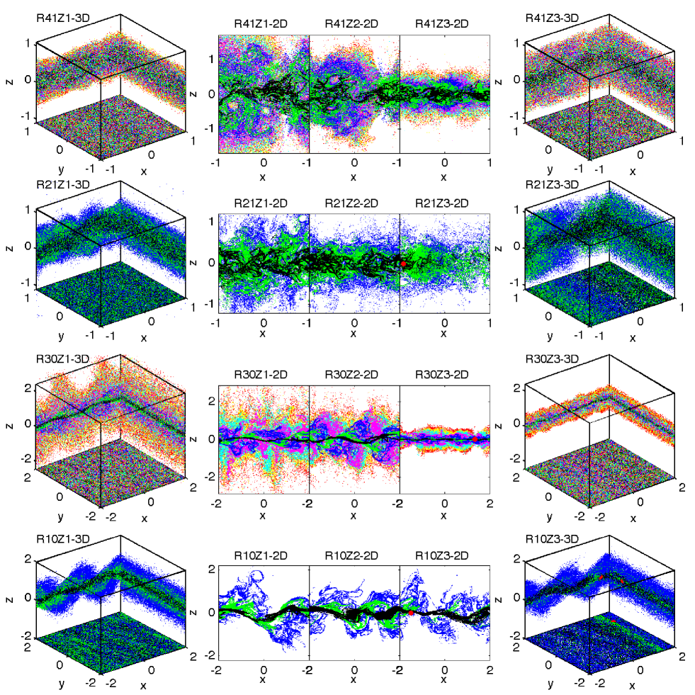
Figure 2.— The distribution of particles at the end of all our simulations. For each 3D run (shown in the leftmost and rightmost panels), we show the projected positions of a subset of particles in three orthogonal directions, while each 2D run is shown in one panel in the center. Different particle species are marked with different colors, and the color coding is the same as that used in Figure 1. Large red dots in a few plots (corresponding to the simulation runs that exhibit strong particle clumping) indicate the densest point in the particle clump. The unit of length in all panels is $\eta r$. Note that the vertical size of our simulation box is larger than shown in this figure.

3. Vertical Structure of the Dusty Midplane Layer

3.1. Kelvin-Helmholtz Instability or Streaming Instability?

The source of turbulence responsible for stirring up the particles can in principle be due to both KHI and SI. It is important to decipher which instability is the dominant process. Generally speaking, the onset of SI requires the averaged particle to gas mass ratio $\epsilon\gtrsim 1$. The strength of the instability decreases as the averaged particle size becomes smaller, and vanishes as $\tau_{s}\rightarrow 0$, for which the dust and gas behave as a single fluid. The onset of KHI requires a steep vertical profile of gas azimuthal velocity, which generally corresponds to larger dust to gas mass ratio at disk midplane. In our simulations, a substantial fraction of the particles have a relatively large stopping time with $\tau_{s}>10^{-2}$, and SI clearly plays an important role in the generation of disk midplane turbulence. It remains to study whether KHI is present and whether KHI is dynamically important.

The classical result on the onset of KHI in a vertically stratified disk is based on the Richardson number criteria (Chandrasekhar, 1961)

$$Ri_{x,y}\equiv\frac{g}{\rho}\ \frac{(\partial\rho/\partial z)}{(\partial u_{x,y}/\partial z)^{2}}\ ,$$ (11)

where we define the Richardson number from radial and azimuthal velocity shear, as indicated by subscripts $x,y$. In the above equation, $g=\Omega^{2}z$ is the vertical gravitational acceleration, and $\rho$ is the effective fluid density (see discussion below). The Richardson number measures the amount of work required to overturn the fluid (numerator) in comparison to the amount of free energy available in the vertical shear (denominator). For Cartesian flow with no rotation, the necessary condition for instability is given by $Ri<Ri^{\rm crit}=1/4$. This criteria no longer holds when rotation (Coriolis force) and radial shear (differential rotation) are included, especially when the rotation frequency $\Omega$ is comparable to the Brunt-V$\ddot{\rm a}$is$\ddot{\rm a}$l$\ddot{\rm a}$ frequency of buoyant oscillations. Generally speaking, the Coriolis force distablizes the fluid (Gómez & Ostriker, 2005), while radial shear acts to stablize the fluid. Lee et al. (2010a) found that $Ri^{\rm crit}$ is typically smaller than $1/4$ and is roughly proportional to dust to gas mass ratio at disk midplane. In this paper, we adopt the critical Richardson number to be $Ri^{\rm crit}=0.1$ as suggested by Chiang (2008).

The Richardson number criterion is based on a single-fluid, in which case $\rho$ simply represents fluid density. With the addition of perfectly coupled dust, the dust-gas system behaves as a single fluid, where the dust contributes to the mass but not the pressure of the fluid, thus $\rho=\rho_{g}+\rho_{p}$. When particles are not perfectly coupled, the definition of $\rho$ becomes somewhat ambiguous, but we expect $\rho_{g}<\rho<\rho_{g}+\rho_{p}$. Below we provide a simple formula for $\rho$ in this regime that reduces the above two limiting cases when $\rho_{p}=0$ and when $\tau_{s}\rightarrow 0$.

In the absence of any turbulence and vertical gravity, the equilibrium state between gas and dust (with fixed stopping time) is described by the NSH solution (Nakagawa et al., 1986). In particular, the azimuthal gas velocity relative to Keplerian velocity is given by

$$u^{\prime}_{y}=-\bigg{[}1-\frac{\epsilon(1+\epsilon)}{(1+\epsilon)^{2}+\tau_{s}^{2}}\bigg{]}\eta v_{K}\ .$$ (12)

where $\epsilon=\rho_{p}/\rho_{g}$, and prime means Keplerian velocity is subtracted. For convenience, we define $\Delta u_{y}\equiv-u^{\prime}_{y}$. For perfectly coupled particles, $\tau_{s}=0$ and we find $\rho_{g}+\rho_{p}=\rho_{g}\eta v_{K}/\Delta u_{y}$. For particles with finite stopping time, $\Delta u_{y}$ becomes closer to $\eta v_{K}$, which reflects the fact that the particle-gas coupling is weaker so that gas velocity shifts towards the dust-free value. Therefore, $\Delta u_{y}$ can be regarded as an indicator of particle-gas coupling. In this spirit, we define the effective gas density as

$$\rho^{\rm eff}\equiv\rho_{g}\frac{\eta v_{K}}{\Delta u_{y}}\ .$$ (13)

It is trivial to check that in the limit $\epsilon\rightarrow 0$, $\rho^{\rm eff}\rightarrow\rho_{g}$, and $\rho^{\rm eff}\rightarrow\rho_{g}+\rho_{p}$ when $\tau_{s}\rightarrow 0$. In the calculation of the Richardson number, we substitute $\rho$ by $\rho^{\rm eff}$. Since $\rho_{g}$ is nearly constant over the height of our simulation box, equation (11) becomes

$$Ri_{x,y}=-\frac{\Omega^{2}z}{\Delta\overline{u}_{y}}\frac{(\partial\overline{u}_{y}/\partial z)}{(\partial\overline{u}_{x,y}/\partial z)^{2}}\ ,$$ (14)

where the overbar means averaging over the horizontal plane. Note that $Ri$ depends on $z$.

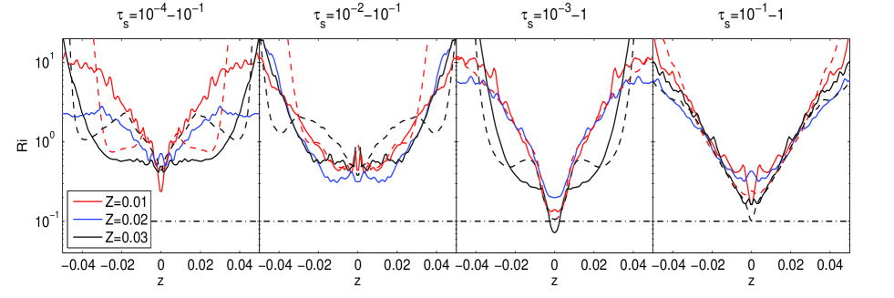
Figure 3.— Profiles of the Richardson number computed from the gas azimuthal velocity from all simulations. Each panel shows the results from one series of runs. Red, blue and black curves label 2D simulations with $Z=0.01,0.02$ and $0.03$ respectively. The corresponding 3D simulations results are marked with the same colors but using dashed lines. Horizontal dash-dotted line marks the critical Richardson number $Ri=0.1$ adopted from Chiang (2008).

Before calculating the Richardson number profile from our simulations, we first return to the spatial distribution of particles in Figure 2. In 2D simulations, we see that the distribution of particles around the disk midplane is highly non-uniform, and exhibit wave patterns in the $x-z$ plane that are almost stationary over time. Results from 3D simulations show very similar features in the $x-z$ plane. In particular, in runs R30Z1-3D and R10Z1-3D, there is a clear segregation of particles with different stopping times, and their wave patterns have a phase shift relative to each other. However, in the $y-z$ plane, there is no coherent structure in the projected distribution of particles in any of our 3D simulations. This contrasts with the expectations from the KHI, where the particle layer kinks and breaks into clumps (Johansen et al., 2006a; Barranco, 2009). Based on this observation, we infer that in our 3D simulations, KHI is not present in the azimuthal direction. Moreover, in the $x-y$ plane, we see azimuthally elongated stripes of the large particles (in black). This feature, together with the standing wave structure in the $x-z$ plane, is most likely to be due to SI. KHI resulting from the vertical shear in the gas radial velocity is another possibility, however, we have found that $Ri_{x}$ is always larger than $Ri_{y}$ from our simulations, therefore the KHI is unlikely to play a role in the simulations presented here.

In Figure 3 we show the Richardson number profile associated from $u_{y}$ calculated from the saturated states of all our simulations. The Richardson number is generally smallest in the disk midplane, and increases with height. In almost all our 3D simulations (dashed curves), $Ri_{y}$ is greater than the critical value (0.1), therefore, the dusty midplane layer is expected to be stable against vertical shear, consistent with the spatial distribution of particles discussed above. Given the fact that $Ri$ does not solely determine stability, this observation does not entirely exclude the possibility that $Ri_{y}$ could be maintained by KHI. However, it is important to note that KHI is suppressed in 2D. We see that $Ri_{y}$ from all our 2D simulations (solid curves) are generally close to their 3D counterpart. This means that the SI itself is able to maintain $Ri$ above the critical value, and suggests that the KHI is indeed absent in all our simulations.

The main reason that we do not observe KHI is that the turbulence generated from the SI is strong enough to prevent particles from settling sufficiently to trigger KHI. We note that the strength of the SI turbulence decreases as the particle stopping time $\tau_{s}$ decreases (as expected from the linear analysis of Youdin & Goodman, 2005, and as confirmed by our numerical experiments). The turbulence in our simulations is mainly generated from relatively large particles with $\tau_{s}\gtrsim 0.01$ (see also the next subsection). We have not explored the regime where all particles are strongly coupled to the gas. However, in this regime, we expect the SI to be generated on much smaller spatial scales with much lower amplitude, so that the particles settle until the KHI is triggered. In this regime, the dust-gas system behaves as a single fluid, where the dust contributes to the mass density but not the pressure of the fluid. This is the approach adopted by Chiang (2008), Barranco (2009) and Lee et al. (2010a, b) to study the KHI.

3.2. Density Profile and Vertical Transport

Figure 4 shows the vertical density profiles for particles of different types from all our 3D simulations, calculated by binning the particles into vertical grid cells and averaging over time after saturation. Results from 2D simulations are generally similar.

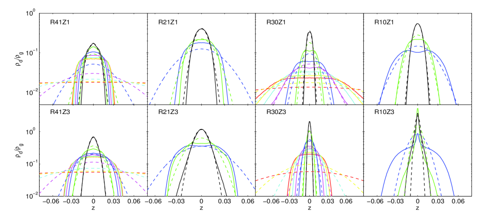
Figure 4.— Vertical profiles of particle density from all our 3D simulations. Profiles of different particle types are labeled with different colors, with the same color scheme as in Figure 1, and particles with smaller stopping time have more extended profiles (see Table 1 for reference). Solid lines are time averaged particle density profiles from the saturated states of our runs, while dashed curves are model density profiles by assuming a constant turbulent diffusion coefficient fits to the density profile of particles with largest stopping time. See §3.2 for details.

Table 2Vertical diffusion coefficient

Run	$Z$	$D_{g,z}$ (2D)	$D_{g,z}(3D)$
	0.01	$2.05\times 10^{-5}$	$1.51\times 10^{-5}$
R41	0.02	$1.72\times 10^{-5}$	-
	0.03	$5.09\times 10^{-6}$	$0.90\times 10^{-5}$
	0.01	$2.12\times 10^{-5}$	$1.42\times 10^{-5}$
R21	0.02	$1.05\times 10^{-5}$	-
	0.03	$1.97\times 10^{-6}$	$1.57\times 10^{-5}$
	0.01	$5.14\times 10^{-5}$	$4.82\times 10^{-5}$
R30	0.02	$1.14\times 10^{-4}$	-
	0.03	$6.28\times 10^{-6}$	$1.21\times 10^{-5}$
	0.01	$1.91\times 10^{-4}$	$1.10\times 10^{-4}$
R10	0.02	$2.44\times 10^{-4}$	-
	0.03	$5.63\times 10^{-5}$	$3.03\times 10^{-5}$

The diffusion coefficients are measured in unit of $c_{s}H_{g}$.

The vertical density profile of particles is determined by the balance between particle settling and turbulent diffusion. Unlike studies of passive particles under the influence of homogeneous external turbulence (Cuzzi et al., 1993; Youdin & Lithwick, 2007), the turbulence from our simulations is self-generated, and is non-homogeneous (strongest at the disk midplane). To study the properties of turbulent diffusion, one approach would be to assume some functional form for the vertical profile of the diffusion coefficient $D_{g,z}(z)$, and fit the particle density profiles. However, after several experiments we found it difficult to fit the density profile of all particle species simultaneously with any simple functional form of $D_{g,z}(z)$ . In fact, the wave patterns in the $x-z$ plane shown in Figure 2 suggests that the classical turbulent diffusion scenario may be too simple.

Instead of fitting the vertical profile of the turbulent diffusion coefficient in the gas, we pose the question in another way: What is the effective vertical diffusion coefficient at the disk midplane for the particles that are driving the turbulence? Since we have identified the SI as the source of the midplane turbulence, one expects particles with relatively large stopping times to drive the turbulence both from a theoretical point of view (Youdin & Goodman, 2005) and from non-stratified simulations of SI (Johansen & Youdin, 2007, Bai & Stone, unpublished). To address these questions more quantitatively, we find the following approach particularly useful.

We fit the horizontally averaged vertical density profile of the largest particles $\tau_{s}=\tau_{\rm max}$ in each simulation using the classical picture of turbulent diffusion. Since these particles (as well as particles with slightly smaller $\tau_{s}$) actively drive the disk turbulence, the gas turbulent diffusion coefficient across this particle layer can be regarded as constant. Therefore, the vertical density profile of these particles is expected to be Gaussian, with scale height (Youdin & Lithwick, 2007)

$$H_{p}(\tau_{s})=\sqrt{\frac{D_{g,z}(0)}{\Omega\tau_{s}}}\sqrt{\frac{\tau_{s}+\tau_{e}}{\tau_{s}+\tau_{e}+\tau_{s}\tau_{e}^{2}}}\ ,$$ (15)

where $\tau_{e}=\Omega t_{\rm eddy}$ is the turnover time of largest eddies. The basic assumption behind this formula is stochastic turbulent forcing on passive particles with the autocorrelation function of the turbulence $P(t)=\exp{(-t/t_{\rm eddy})}/2\pi$, corresponding to a Kolmogorov spectrum. We do not have much knowledge of $t_{\rm eddy}$ for SI turbulence, but expect it to be comparable to the orbital time (the only time scale of the problem), and take $\tau_{e}=1$. The exact value of $\tau_{e}$ does not matter much, since it only gives an order unity correction to $H_{p}$.

By fitting the vertical density profile of the largest particles with a Gaussian we obtain $D_{g,z}(0)$ for all simulations, and the results are summarized in Table 2. For 3D runs, the results are also plotted in Figure 4 as dashed lines. We see that the vertical profiles of the largest particles are well fitted with a Gaussian. In addition, we predict the vertical density profile for other particle species, using equation (15) and assuming a diffusion coefficient which is constant with height. Obviously, this will overpredict the scale heights for small particles, since they respond to the turbulence passively. However, for particles that actively participate in the instability, we expect their density profile to be comparable to the predicted profile, since they are driving turbulence to maintain $D_{g,z}$ close to $D_{g,z}(0)$ across their scale heights. In this way, we are able to identify the particle species that are responsible for the disk turbulence (hereafter termed as “active” particles).

From the R41 runs, we see that active particles range from $\tau_{s}=0.1$ (for R41Z1) to $\tau_{s}\gtrsim 0.01$ (R41Z3). Active particles for R21 runs have $\tau_{s}\gtrsim 0.03$. For R30 runs, particles with $\tau_{s}\gtrsim 0.03$ are active, while for R10 runs, all particles are active. We see that although there is a diversity in the size range of active particles, which depends on both solid abundance and particle size distribution, the minimum size of active particles for most of our runs is about $\tau_{s}=0.01-0.03$. For run R41Z1, although we have identified somewhat larger $\tau_{s}$ values for active particles, particles with $\tau_{s}=0.01-0.1$ must actively participate in the instability because the abundance of $\tau_{s}=0.1$ particles alone is too small to trigger SI.

Next we study the midplane diffusion coefficient from our simulations. We emphasize that the strength of the turbulence (hence $D_{g,z}$) is self-regulated: the settling of particles continues until the turbulence they generate is sufficient to stop the settling. To better interpret our results, we construct a toy model describing the self-regulated turbulence. In this model, we assume all particles are active, and that the particles are single-sized, with fixed stopping time $\tau_{s}$. Since all particles are active, their vertical density profile can be approximated by a Gaussian, so that the particle to gas mass ratio at the disk midplane is given by $\epsilon=ZH_{g}/H_{p}$. The midplane diffusion coefficient $D_{g,z}$ depends on both $\tau_{s}$ and $\epsilon$. For simplicity, we parameterize the dependence as

$$D_{g,z}=\epsilon^{\alpha}f(\tau_{s})H_{g}^{2}\Omega\ ,$$ (16)

where $D$ is normalized to $H_{g}^{2}\Omega$, $f(\tau_{s})$ is a coefficient that incorporates the dependence of $D$ on $\tau_{s}$, and $\alpha$ is a power law index that reflects the sensitivity of the dependence of $D$ on $\epsilon$. We note that $D_{g,z}\rightarrow 0$ at both $\epsilon\rightarrow 0$ and $\epsilon\rightarrow\infty$, therefore, we expect $\alpha>0$ when $\epsilon$ is small and $\alpha<0$ for large $\epsilon$. Using equation (15) and neglecting the second square root (which is order unity) on the right hand side, we obtain

$$\begin{split}H_{p}=&\bigg{(}\frac{f}{\tau_{s}}Z^{\alpha}\bigg{)}^{\frac{1}{2+\alpha}}\cdot H_{g}\ ,\\ D_{g,z}=&(fZ^{\alpha})^{\frac{2}{2+\alpha}}\tau_{s}^{\frac{\alpha}{2+\alpha}}\cdot H_{g}^{2}\Omega\ .\\ \end{split}$$ (17)

In the above equations, the dependence of particle scale height and diffusion coefficient on $Z$ is reflected in the index $\alpha$. When $\alpha$ is positive, increasing $Z$ leads to larger $H_{p}$ and larger $D_{g,z}$. When $\alpha$ is negative, the situation reverses. Below, we apply this simple model to our results. Since our simulations contain multiple particle species, we may take $\epsilon$ to represent the contribution from all particle species participating in the SI (i.e. with $\tau_{s}\gtrsim 0.01$).

Our R30 and R10 runs show similar behavior between 2D and 3D simulations with respect to vertical diffusion properties. Increasing $Z$ from 0.01 to 0.02 produces stronger turbulence, while further increasing $Z$ to 0.03 dramatically reduces $H_{p}$. This corresponds to the transition from $\alpha>0$ to $\alpha<0$ at a threshold $\epsilon$ (hence threshold $Z=Z_{\rm th}$). Beyond $Z_{\rm th}$, $H_{p}$ sensitively depends on $Z$ because the corresponding power law index $\alpha/(2+\alpha)$ quickly drops to large negative values once $\alpha$ turns negative. Consequently, a small increase in $Z$ results in strong particle settling and greatly enhances midplane particle density. This result has important implications for particle clumping discussed in the next section.

In our 2D R41 and R21 runs, we see that $D_{g,z}$ monotonically decreases with $Z$, suggesting $\alpha<0$ for $Z\geq 0.01$. Based on this result, we infer that the strength of the SI for a particle size range $\tau_{s}=0.01-0.1$ is a decreasing function of $\epsilon$ for $\epsilon\gtrsim 0.5$. The 3D simulations give somewhat different results. For both 3D R41 and R21 runs, $D_{g,z}$ slightly increases with $Z$ at least in the range $Z\leq 0.03$, indicating $\alpha\geq 0$. It is very likely that the threshold abundance $Z_{\rm th}$ is above $0.03$, which is substantially larger than their 2D counterparts. We note that the behavior of the SI turbulence for $\tau_{s}\lesssim 0.1$ particles in 3D is different from that in 2D in non-stratified simulations (Johansen & Youdin, 2007). Our results indicate that the difference remains when vertical gravity is included, and 3D simulations are needed to better catch the dynamics of small particles.

In our toy model, all of our ignorance on the dependence of $D_{g,z}$ on $\tau_{s}$ is encapsulated in the unknown function $f(\tau_{s})$. From Table 2 we see that the R30 and R10 runs generally have larger $D_{g,z}$ than R41 and R21 runs. This result implies that turbulence generated from larger particles $\tau_{s}\sim 1$ is stronger than that from smaller particles, i.e., $f(\tau_{s})$ is an increasing function of $\tau_{s}$ in this range, consistent with results from non-stratified simulations (Johansen & Youdin, 2007).

In sum, we have identified that particles actively participating in SI generally have stopping time $\tau_{s}\gtrsim 0.01$. The strength of the turbulence largely depends on the density of these active particles at disk midplane. We find that the particle scale height (thus the turbulent diffusion coefficient) strongly depends on solid abundance. Such strong dependence is caused by a sharp drop in the strength of the turbulence with increasing particle to gas mass ratio $\epsilon$ when $\epsilon$ is larger than a certain threshold value.

4. Particle Concentration

4.1. Formation of Particle Clumps

Probably the most interesting property of the SI is the concentration of particles. The degree of particle concentration strongly depends on the mass distribution of solids in PPDs. In our simulations, we normalize particle density to the background gas density at the disk midplane $\rho_{g,b}(r,z=0)$. A useful scale to measure particle concentration is the Roche density, above which the particle clump can be considered as gravitationally bound (Binney & Tremaine, 2008)

$$\rho_{\rm roche}(r)\approx\frac{3M_{*}}{r^{3}}=1.34\times 10^{3}\frac{(f_{M}f_{T})^{1/2}}{f_{g}}r_{\rm AU}^{\frac{2b-c-3}{2}}\rho_{g,b}(r,0)\ .$$ (18)

The normalized Roche density (relative to the background gas density at midplane) scales as the square root of stellar mass and disk temperature, and is inversely proportional to disk mass, meaning that the Roche density is easier to reach for massive disks (with large $f_{g}$). In the MMSN model, the Roche density is of the order $\rho_{\rm roche}=10^{3}\rho_{g,b}$, and only weakly depends on $r$ as $r^{-1/4}$.

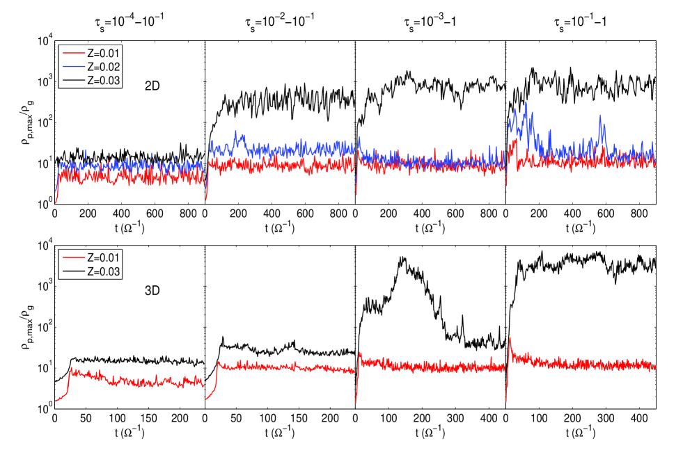
Figure 5.— The evolution of maximum particle density for all our simulations. Each panel shows the results from one run series. In the upper panels, red, blue and black curves label 2D simulations with $Z=0.01,0.02$ and $0.03$ respectively. The 3D results are shown in the lower panels with $Z=0.01$ and $0.03$ marked with red and black. The maximum density is normalized with respect to the background gas density at the disk midplane.

In Figure 5 we show the time evolution of maximum particle density $\rho_{p,{\rm max}}$ from all our simulations. We first look at results from 2D simulations. For all the four run series, $\rho_{p,{\rm max}}$ increases with solid abundance $Z$. However, the dependence of $\rho_{p,{\rm max}}$ on $Z$ is highly non-linear. For run series R21, R30 and R10, there is no significant clumping of particles for $Z=0.01$ and $0.02$. However, significant clumping occurs at $Z=0.03$, with maximum particle density reaching $10^{3}$ times the background gas density, comparable to the Roche density (18). This trend is consistent with the results by Johansen et al. (2009) (see also the supplemental information in Johansen et al., 2007), who considered particles with stopping time in the range of $\tau_{s}=0.1-0.4$. As emphasized in the previous section, there is a sharp enhancement of averaged midplane particle density with increasing $Z$ once $Z$ exceeds some threshold value. This density enhancement further favors strong concentration of particles by SI, which explains the trend we have observed in Figure 5.

The particle clumping also depends on the particle size distribution. In the R41 run series, where the majority of the particle mass resides in strongly coupled particles $\tau_{s}<10^{-2}$, we see that there is no significant clumping of particles up to $Z=0.03$. As noted in the previous section, particles that effectively participate in SI are those with relatively large stopping times $\tau_{s}\gtrsim 10^{-2}$. These particles are also the ones that actively participate in the clumping (see the next subsection). For R41 runs, the abundance of these “active” particles is much smaller than our R21, R30 and R10 runs, which makes the critical (total) abundance for strong particle clumping larger. In fact, we do observe strong clumping when we increase the total abundance to $Z=0.05$. Based on the discussion above, we conclude that in order for the SI to efficiently concentrate particles, the mass of the solids with stopping time $\tau_{s}\gtrsim 10^{-2}$ should exceed a critical value $Z_{\rm crit}$. The results from 2D simulations suggest that $\sum_{\tau_{k}\geqslant 10^{-2}}Z_{k}\gtrsim Z_{\rm crit}\approx 0.02$ is necessary for significant particle clumping.

The 3D simulations show similar trends as in 2D, but the condition for strong particle clumping is more stringent. Among the eight 3D runs, strong clumping occurs only in run R10Z3-3D. The maximum density for all other runs remain small in the saturated state ($\rho_{p,{\rm max}}\lesssim 50\rho_{g,b}$). In particular, the 3D R21Z3 and R30Z3 runs do not show clumping as in their 2D counterparts, and both of them have larger $D_{g,z}$. Since KHI is unlikely to be present in these simulations, the different results between our 2D and 3D simulations should be attributed to the different behavior of the SI in 2D and 3D. It appears that the formation of dense particle clumps favors the mass distribution of particles to be dominated by larger particles than in 2D, or larger values of $Z_{\rm crit}$ is needed.

Interestingly, in run R30Z3-3D, a very dense clump (actually a nearly axisymmetric stripe) forms at about $t=150\Omega^{-1}$. The composition of this (transient) clump is similar to its counterpart R30Z3-2D (see next subsection). It lasts for about 10 orbital times and then is gradually dissolved. Both the Richardson number profile and particle distribution disfavor the presence of KHI during the process. Nor is there any significant vorticity generation in the vicinity of the clump which might indicate KHI. By comparing with Figure 1, we see that the period during which the clump is dissolved is accompanied by an increase of the height of relatively small particles with $\tau_{s}\lesssim 0.1$. It is likely that the formation of the transient clump is due to our unrealistic initial condition.

The results we have obtained show a clear dichotomy on the particle concentration properties. Specifically, the maximum density is either very small with $\rho_{p,{\rm max}}\lesssim 50\rho_{g,b}$, or very large with $\rho_{p,{\rm max}}\gtrsim 1000\rho_{g,b}$. Self-gravity becomes important when the particle density approaches the Roche density (18). This means that for our simulations that do not show signature of strong clumping, adding self-gravity will not change the picture qualitatively. For simulations with strong clumping, the maximum particle density is already comparable with the Roche density, and in this case we expect the formation of a few planetesimals from the simulations as in Johansen et al. (2009).

Particle concentration properties are known to depend on numerical resolution. To assess the validity of our results, we have also performed the same set of simulations with half our standard resolution. We find the same dichotomy between strong clumping and no clumping. The only exception is the R30Z3-3D run: it shows strong particle clumping in the low-resolution run which does NOT dissolve as in our standard resolution run. The reason is that the turbulence generated from the lower resolution run is weaker, thus particles settle more which favors clumping. This test justifies the necessity of conducting high resolution simulations. In the mean time, it suggests that the critical abundance for particle clumping in this run may be only slightly larger than $0.03$. Therefore, the particle clumping properties from 2D and 3D simulations is not dramatically different when $\tau_{\rm max}=1$.

4.2. Properties of Dense Clumps

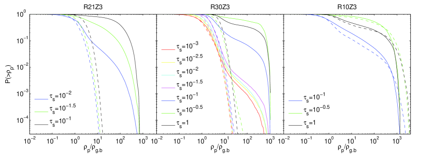
Figure 6.— The cumulative probability distribution function (CPDF) of particle densities in the saturated state from the three simulations that exhibit strong particle clumping. Different colors mark the CPDF of different particle species, as labeled in the legend. Solid curves come from 2D simulations, while results from 3D simulations are denoted in dashed curves. Particle densities are normalized to background gas density at disk midplane.

In this subsection we discuss more details of the three simulations that exhibit strong particle clumping. First, we examine the composition of these dense clumps by plotting the cumulative probability distribution function (CPDF) of particle densities for different particle species $P(\rho_{p}>\rho)$. The CPDF measures the probability of a particle residing in a region with total particle density larger than $\rho$. In Figure 6, we plot the CPDFs of the three runs: R21Z3, R30Z3 and R10Z3. At relatively high densities with $\rho_{p}\gtrsim 10^{2}\rho_{g}$, we see that in all three cases, the dense regions are composed of particles with the largest stopping times. In run R21Z3-2D, the mass fraction of different particle species in the dense clumps is increasing with particle stopping time $\tau_{s}$, and is completely dominated by the largest particles $\tau_{s}=0.1$. In the case of R30Z3-2D and R10Z3-2D, where the largest particles have $\tau_{s}=1.0$, the composition of the clumps are dominated by the two largest particle species. Contribution from other particle species to the clumps is almost negligible by mass.

For R21Z3 and R30Z3 runs, 3D simulations do not show particle clumping, therefore, the resulting CPDFs differ substantially from those in 2D runs. Nevertheless, these CPDFs provide typical examples for simulations without clumping. The shapes of the CPDFs from different particles are very similar, and curves for larger particles are located to the right of those for smaller particles, consistent with the vertical stratification of particles. For run R10Z3-3D, the particle clumping is stronger than the 2D case, and the densest clumps are almost equally made of particles with $\tau_{s}=1$ and $\tau_{s}=10^{-1/2}$.

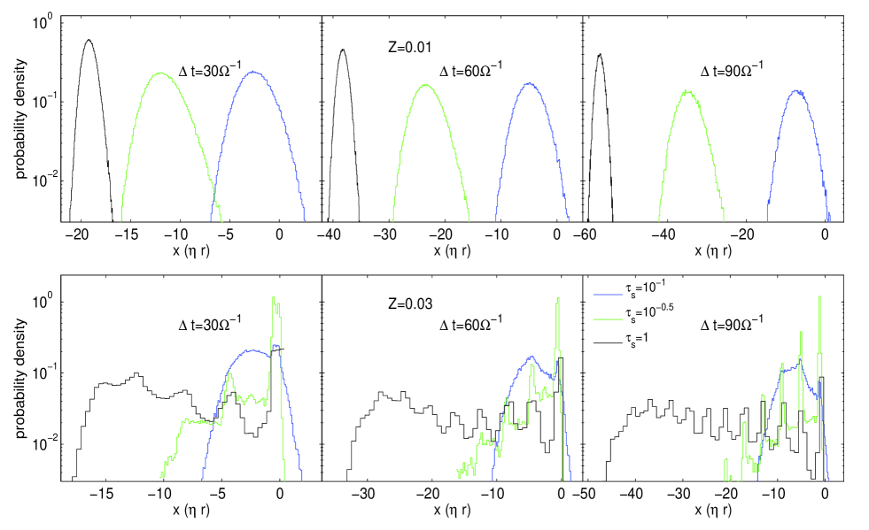
Figure 7.— The probability distribution of the radial distance traveled by various types of particles after a given time interval $\Delta T$ from our runs R10Z1-3D (top) and R10Z3-3D (bottom). We choose $\Delta t=30$, $60$ and $90$ as shown in left, middle and right panels respectively (unit is $\Omega^{-1}$). Particles of different types are labeled by different colors (see the legend).

Next, we consider the motion of the dense clumps. In Figure 2, we mark the location of the densest point with a red dot in runs with strong particle clumping. By monitoring the location of the densest point with time, we find that it wanders slowly. Another useful way of studying the dynamics of the clumps is by tracking the radial trajectories $x_{i}(t)$ of a sample of particles. We relocate the particle positions when they cross the radial boundaries of our simulation box so that their trajectories are continuous. By tracing a large number of particles in the saturated state of our runs, we obtain the distribution of $x(t+\Delta t)-x(t)$ for each particle species at time interval $\Delta t$. In Figure 7 we show the probability distribution of $x(t+\Delta t)-x(t)$ for a number particle species from our run R10-3D. When $Z=0.01$, no particle clumping occurs. The distribution of $x(t+\Delta t)-x(t)$ is close to a Gaussian (or a parabola in logarithmic scale) and the width increases with $\Delta t$, consistent with undergoing a random walk. Meanwhile, the center of the distribution drifts inward with time (see §5 for more discussion). However, when particle clumps are present, as in the $Z=0.03$ case, the shape of the distribution deviates substantially from a Gaussian, especially for particles that make up the clumps (the largest particles, shown in the blue and green curves). For these clump-making particles, the width of particle distribution still increases with $\Delta t$, as expected from turbulent diffusion, but a substantial fraction of theses particles stay nearly stationary without drifting (near $x=0$), making the resulting distribution more and more elongated with time. The leftmost location of the particle distribution moves inward with time, and is set by the radial drift velocity. More interestingly, we see almost evenly separated multiple peaks in the distribution function. In fact, the separation between these peaks equals the radial size of our simulation box. The physical picture becomes clear that the clumps stop some of the particles from drifting radially, and particles are kept in the clump for a few orbits or more before leaving for the next clump. Similar behavior is observed for other runs with particle clumping.

5. Radial Transport of Solid Particles

As expected from particle-gas equilibrium, particles experience head wind from the gas and drift radially inward. Particles with different stopping times drift at different velocities. At the same time, the instabilities generated at the disk midplane diffuse the particles. These two processes transport particles radially in PPDs, and is the subject of this section. In particular, we show that it is important to study the radial transport of particles by considering particles of all sizes simultaneously, rather than individually.

5.1. Radial Drift Velocity

We calculate the averaged radial drift velocities for each particle species from all our runs, and the results are shown in Figure 8. The measured mean drift velocities are shown in squares (2D) and circles (3D). We have also plotted the $1\sigma$ limits for particle drift velocity based on the rms fluctuations, which are indicated in blue and red vertical bars. In the figure, the velocities are normalized to $\eta v_{K}$. Clearly, the radial drift velocity monotonically decreases with particle stopping time, and the drift is fastest for marginally coupled particles.

The classical result on the radial drift of particles is the NSH equilibrium solution (Nakagawa et al., 1986). It describes the equilibrium state between solids and gas in unstratified (neglecting vertical gravity) Keplerian disks, where gas is partially supported by radial pressure gradient. In the NSH equilibrium, the drift speed is given by

$$v_{x}=-\frac{2\tau_{s}}{(1+\epsilon)^{2}+\tau_{s}^{2}}\eta v_{K}\ .$$ (19)

We emphasize that the conventional NSH solution is obtained by considering a single species of solids. Equation (19) does not simply generalize to the case with multiple-species of particles by replacing $\epsilon$ to $\epsilon_{k}$ for each particle species $k$. In Appendix A we provide the generalized formula for multi-species NSH equilibrium, and the solution involves evaluation of an inverse matrix of order $2N_{\rm type}$. It reflects the fact that although different particle species do not interact directly with each other, they are indirectly coupled via their interactions with gas.

In Figure 8, the bold solid lines show the expected radial drift velocities from single-species NSH equilibrium. We see that there are large deviations from the measured mean drift velocities, with two notable features. First, for relatively large particles, the drift velocities are reduced from single-species NSH values. The reduction is strongest for runs with the largest $Z$. Second, the smallest particles drift outward, rather than inward as expected from the single-species NSH solution.

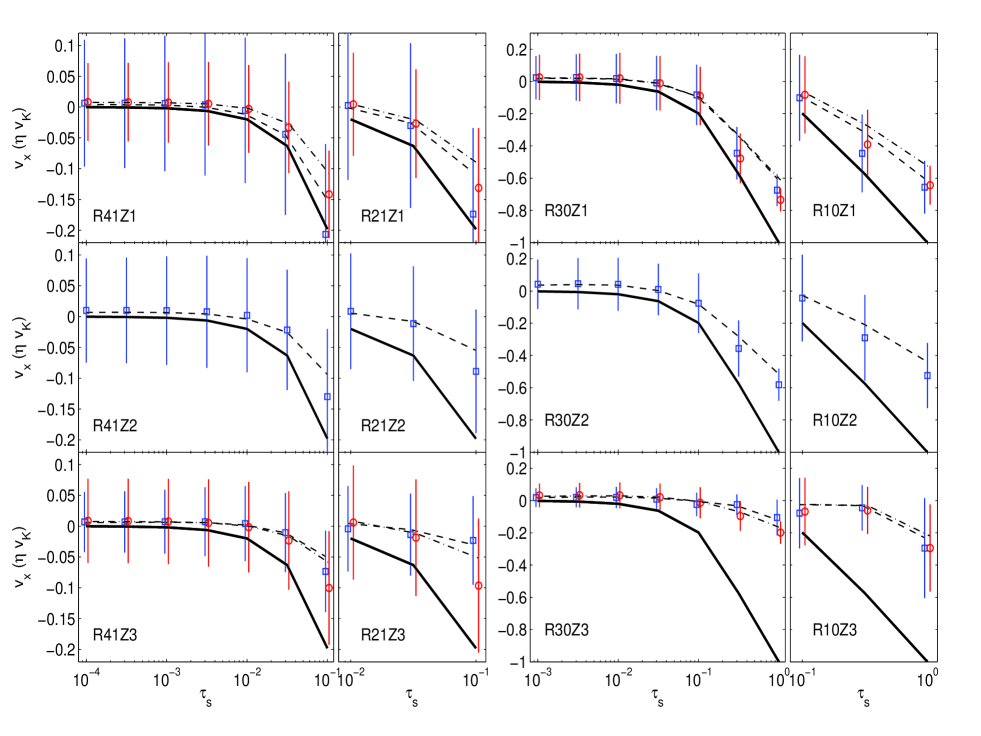
Figure 8.— Radial drift velocities for different particle species from all our simulations. Blue squares: averaged particle radial drift velocity from 2D simulations, and vertical blue bars indicate its $1\sigma$ limits. Red circles: averaged particle radial drift velocity from 3D simulations, and vertical red curves show its $1\sigma$ limits. We have slightly shifted the symbols for 2D and 3D runs in order to show the $1\sigma$ bars more clearly. Bold black solid line: radial drift velocity expected from single-species NSH equilibrium. Black dashed (dash-dotted) line: radial drift velocity expected from multi-species NSH equilibrium (see Appendix A) for 2D (3D) simulations. All velocities are normalized to $\eta v_{K}$.

To calculate the expected radial drift velocity from a multi-species equilibrium, we first use the particle density profiles extracted from §3.2 and calculate the drift velocity in each vertical bin. The drift velocity is then weighted by particle density in each bin to yield the mean drift velocity. The results are plotted in dashed and dash-dotted lines (for 2D and 3D runs respectively) in Figure 8. We see that these curves provide an excellent fit to the measured mean radial drift velocities in all simulations. In fact, the two features mentioned above are natural consequences of the multi-species solution. Due to the sub-Keplerian motion of the gas, particle drag increases gas angular momentum, leading to outward drift of gas. In the presence of both weakly coupled and strongly coupled particles, the strongly coupled particles are tied to the gas and therefore drift outward with the gas. Marginally coupled particles still drift inward, but due to the influence of the smaller particles, these particles feel a weaker headwind (i.e., the gas azimuthal velocity is closer to the Keplerian value), resulting in a smaller drift velocity compared with the single-species solution. With increasing $Z$, thus higher midplane particle density, the gas becomes more entrained by the solids, leading to stronger reduction of the drift velocity for large particles.

The residuals from the multi-species NSH solution fit to the measured mean drift velocities are largest for particles with largest $\tau_{s}$, likely due to their participation in SI, and/or clumping. In the non-stratified simulation of Johansen & Youdin (2007), it was shown that in the saturated state of SI, the radial drift velocity is either increased or decreased depending on run parameters. In our simulations, these effects are secondary compared with the multi-species effect. The measured drift velocities from 2D (squares) and 3D (circles) simulations generally agree with each other. The (small) differences can be attributed to the differences in the particle vertical density profiles.

So far we have focused on the mean radial drift velocities. In the saturated state of our simulations, the particle radial drift velocities follow a distribution, due to the SI. We see in Figure 8 that in most of the runs, the fluctuation level is about $(0.05-0.15)\eta v_{K}$. This fact is closely related to the radial diffusion of particles discussed in the next subsection. Based this observation, we can estimate the particle radial diffusion coefficient to be $D_{x}\sim(0.1\eta v_{K})^{2}/\Omega\sim 2.5\times 10^{-5}c_{s}H_{g}$.

5.2. Radial Diffusion

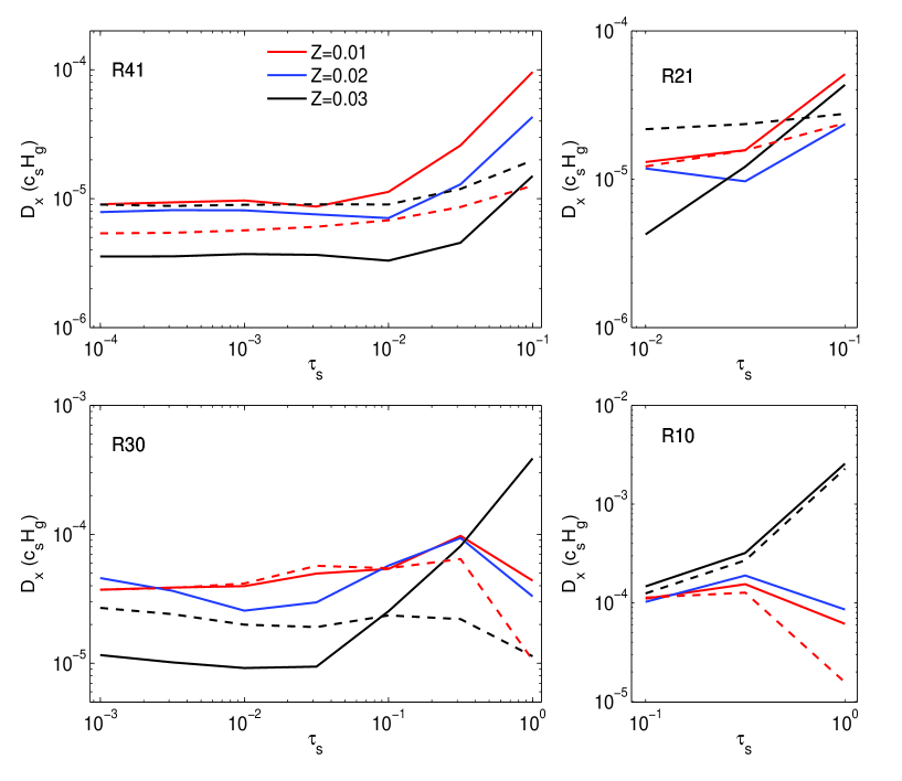
Figure 9.— Radial diffusion coefficient for different particle species from all our simulations. Results from 2D and 3D simulations are shown in solid and dashed lines respectively. Red, blue and black curves represent different metallicities with $Z=0.01,0.02$ and $0.03$ respectively. Diffusion coefficients are normalized by $c_{s}H_{g}$.

The radial diffusion of particles is generally characterized by the radial diffusion coefficient $D_{x}$. From our simulations, we can measure $D_{x}$ for different particle species based on the random walk model of particle diffusion. We calculate the distribution of shift in the particle radial position at various time intervals $\Delta t$ as in Figure 7, and measure the width (rms) of the distribution $\sigma$ as a function of $\Delta t$. The spreading due to a random walk results in an Gaussian distribution, and $\sigma$ is related to the diffusion coefficient by

$$D_{x}=\frac{1}{2}\frac{d\sigma_{x}^{2}}{dt}\ ,$$ (20)

For each particle species, we measure $\sigma_{x}^{2}$ for different $\Delta t$, and fit the slope in of the $\sigma^{2}-\Delta t$ curve by linear regression. The results are summarized in Figure 9. The range of the radial diffusion coefficient is consistent to within an order of magnitude of the estimate in the last subsection based on the spread of radial drift velocities. It is also comparable with the vertical diffusion coefficient at disk midplane estimated in §3.2 (see Table 2). Below we discuss these results further.

First, the above procedure for measuring the diffusion coefficient does not apply to runs that show strong particle clumping. As we see in Figure 7, the distribution of $x(t+\Delta t)-x(t)$ deviates strongly from a Gaussian due to the influence of the clumps. The measured width of the distribution is about half the distance traveled by the fastest drifting particles (those that are not confined in the clumps), and we observe that $\sigma_{x}^{2}$ scales as $\Delta t^{2}$ rather than $\Delta t$ from our measurement. Therefore, the measured $D_{x}$ from R21Z3-2D, R30Z3-2D and R10Z3 (both 2D and 3D) runs for those clump making particles (or the largest two particle species in the run) is not valid. In Figure 9, we see the measured $D_{x}$ for these particles have anomalously large values. Such particles can reside in the disk for much longer than if there were no clumping.

Next, we discuss diffusion of non-clumping particles. In each simulation the measured $D_{x}$ generally approaches an asymptotic value for particles with $\tau_{s}\lesssim 10^{-2}$, but is different between different particle species for particles with $\tau_{s}>10^{-2}$. This can be due to multiple reasons. First, similar to the vertical diffusion of particles, the radial diffusion coefficient also depends on the vertical position in the disk, and the radial diffusion in the disk midplane is expected to be the strongest. Our measured $D_{x}$ can be considered as a vertically averaged quantity. Therefore, $D_{x}$ is expected to be larger for particles with larger $\tau_{s}$, since they stay closer to the midplane. This trend is observed in runs R41 and R21. Second, different particles react differently to the turbulence. In the case of Kolmogorov turbulence, the particle diffusivity scales as $(1+\tau_{s}^{2})^{-1}$ (Youdin & Lithwick, 2007). This may be responsible for the decrease of $D_{x}$ towards $\tau_{s}=1$ in R30 and R10 runs with $Z=0.01$ and $0.02$. Thirdly, different particles participate in the SI in different ways (i.e., actively or passively). The SI may strongly affect the transport properties of the active particles, with the extreme example being the clump-making particles discussed above. Despite the different values of $D_{x}$ for different particle species, one may take the asymptotic value of $D_{x}$ as measured from the smallest particles as characteristic of the radial diffusion coefficient in the gas. These asymptotic values correlates with the vertical diffusion coefficient well (see Table 2).

To address the effectiveness of radial diffusion compared with radial drift, we denote the mean radial drift velocity to be $v_{r}=\kappa\eta v_{K}$, and the diffusion coefficient to be $D_{x}=(\beta\eta v_{K})^{2}/\Omega$. After time $t$, the ratio

$$\zeta\equiv\frac{v_{r}t}{\sigma(t)}=\frac{\kappa}{\beta}\sqrt{\Omega t/2}\ ,$$ (21)

reflects the relative importance between radial drift and turbulent diffusion, where $\sigma(t)=\sqrt{2D_{x}t}$. Diffusion is important when $\zeta\lesssim 1$. From Figure 8, we see that for the largest particles, $\kappa\gtrsim 0.1$. From Figure 9, we have $\beta\lesssim 1$. Therefore, the effect of radial diffusion of particles becomes negligible compared with radial drift beyond $100$ orbital periods. Again, this discussion does not apply to the situation when particle clumping is present, where large particles can be retained in the clumps and some of them may survive the radial drift.

6. Collision Velocities

The initial stage for planetesimal formation is the growth of solid bodies by mutual collisions. The size distribution of particles in the PPDs therefore depends on the outcome of two-body collisions, which further depends on the properties of the colliding particles (e.g., size and porosity) and collision velocity. Laboratory experiments show that at low collision velocities ($\lesssim 1$m$\cdot$s^-1), collisions generally lead to sticking or bouncing. Larger collision velocities tend to result in fragmentation (see the review by Blum & Wurm, 2008). Nevertheless, sticking can also occur with collision velocities up to $10-20$m$\cdot$s^-1 in some regimes (see Figure 11 of Güttler et al., 2009). The particle size distributions used in this paper can be considered as a first approximation to the outcome of grain growth in PPDs. In turn, we can measure the two-body collision velocity produced by the SI from our simulations and investigate whether our selected particle size distribution is consistent with the outcome of collisional coagulation.

We measure the relative speeds of all particle pairs within a distance $\Delta r$ in the saturated state of our simulation snapshots. These velocities form a representative sample of particle relative velocity distribution (RVD) in the vicinity of a tracer particle. We assume that particles that collide with this tracer particle would have the same RVD. The measured RVD depends somewhat on the choice of $\Delta r$. In practice, we choose $\Delta r$ to be a quarter of a cell size, in order to reduce the (misrepresented) measured collision velocity between strongly coupled particles (see Figure 10 and the discussion that follows), while maintaining good statistics. To obtain the distribution of collision velocities with a tracer particle, the RVD must be weighted by the relative velocity, since the collision frequency is enhanced at larger relative velocities. The corresponding CPDFs (similar to §4.2) are shown and discussed in Appendix B. In this context, it measures the probability of a particle that undergoes collision with relative velocity greater than a given value. Particle velocities are normalized to the gas sound speed $c_{s}$ in our simulations. In all the results presented in this section, we adopt $c_{s}=0.99$km s^-1, corresponding to the MMSN model at 1AU.

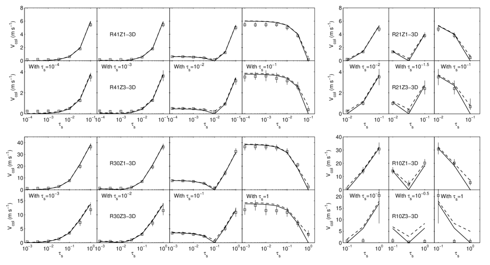
Figure 10.— The median collision velocity for two-body particle collisions from all our 3D simulations. In each subplot, upper panels show results from metallicity $Z=0.01$ and bottom panels for $Z=0.03$. Plotted in each panel are median collision velocities between one particle with fixed $\tau_{s}$ and a second particle as a function of $\tau_{s}$ of the second particle. Squares: measured median collision velocities from the simulations. Vertical bars: the $1\sigma$ range of the collision velocities. Solid lines: expected collision velocity calculated from the radial drift velocities using multi-species NSH equilibrium (see Figure 8). Dashed lines: expected collision velocity from both radial drift and turbulence based on results from Figures 8 and 9 (see text for details). The collision velocities scales linearly with the adopted sound speed, and we take $c_{s}=0.99$km s^-1 appropriate for MMSN model at 1AU.

In order to visualize the particle collision velocities in a compact way, we characterize the CPDFs by the median collision velocity (at $P=0.5$) and its $1\sigma$ limits (at $P=0.68$ and $P=0.32$). In Figure 10 we show the median collision velocities and $1\sigma$ limits for various pairs of particle species from all our 3D simulations. Results from 2D simulations are generally similar, and are not plotted. To interpret these results, we consider two sources of the collision velocities: radial drift and turbulence.

To calculate the contribution from radial drift, we evaluate the multi-species NSH equilibrium in each vertical cell bin $j$ ($j=1,...,N_{z}$), from which we obtain the relative radial drift velocity $(\Delta v_{r})_{k_{1},k_{2}}^{j}$ between each pair of particle types $k_{1},k_{2}$ in that bin. The relative velocity is further weighted by collision frequency in that bin, proportional to $(\Delta v_{r})_{k_{1},k_{2}}^{j}\epsilon_{k_{1}}^{j}\epsilon_{k_{2}}^{j}$. Integrating over all the vertical bins, we obtain the expected collision velocity from radial drift, which is shown as solid curves in Figure 10. We see that with the exception of run R10Z3-3D, these curves fit the median collision velocities very well, meaning that relative radial drift is the dominant source of collision velocities.

R10Z3-3D is the only 3D run that shows strong particle clumping, and the measured median collision velocity is strongly reduced from our predictions. This is clearly seen in the CPDF plot (see Figure 12 in Appendix B). However, in these simulations, the median collision velocity no longer characterizes the overall collision velocities because the shapes of the CPDFs are strongly deformed due to the clumping. In fact, there is still a high-velocity tail in the CPDF of collision velocity, which reaches values as high as $30$m s^-1. This tail is most likely caused by collisions outside the clump, as indicated in Figure 13, and our predicted collision velocities should apply in these low density regions.

The relative radial drift velocity can not account for the collision velocity between particles with the same stopping time (therefore all solid curves reach a zero point in Figure 10). To remedy this limitation, we further consider the contribution from turbulence. So far turbulence induced particle collision velocities has been studied theoretically only in the framework of passive particles in uniform Kolmogorov turbulence (Voelk et al., 1980; Markiewicz et al., 1991), and in MRI turbulence (Carballido et al., 2008). We consider the closed form expression of turbulent collision velocities by Ormel & Cuzzi (2007), which is based on the Kolmogorov spectrum. Although these assumptions do not quite apply in our simulations, we adopt this approach as an approximate treatment of turbulence induced collision velocities. We use their equation (16), and more specifically, we fix the turn over time for the smallest eddy to be $t_{\eta}=0$, and take $y^{*}=t^{*}/t_{\rm stop}=1.6$ as an approximation (where $t^{*}$ is the turn over time of the critical eddy with which the particle in question is marginally coupled). The turn over time of the largest eddy $t_{L}$, is considered as a fitting parameter. Because the strength of the turbulence is vertically stratified, we take the averaged radial diffusion coefficient $D_{x}$ from the smallest particles in each of our simulation run. The averaged gas velocity $V_{g}$ is then related to $D_{x}$ by $D_{x}\simeq V_{g}^{2}t_{L}$.

In Figure 10, we also show the contribution from turbulence induced relative velocities as dashed curves. In order to fit the collision velocity for pairs of large particles $\tau_{s}\gtrsim 0.1$, we find $\Omega t_{L}\simeq 2-3$ for R41 and R21 runs, and $\Omega t_{L}\simeq 4$ for R30 and R10 runs. With this contribution, the collision velocity between the same types of particles can be fit very well, and it also improves the fit to collision velocities between particles with different types.

In our R41 and R31 runs, the predicted collision velocities almost reach zero for collisions between particles with $\tau_{s}\lesssim 10^{-3}$, since contributions from both radial drift and turbulence rapidly decrease with stopping time. The measured collision velocities are always larger than the predicted values, as seen in the leftmost four panels of Figure 10, and decrease towards a small asymptotic value at smallest $\tau_{s}$. We have experimented with choosing different $\Delta r$ in our calculations and found that the asymptotic value roughly scales linearly with $\Delta r$ when $\Delta r$ is less than grid size, because the gas velocity is not resolved at scales less than a grid cell.

From Figure 10, the median collision velocity is typically a fraction of $\eta v_{K}$ ($\sim 50$m s^-1 with our chosen scaling). Since the collision velocity is dominated by the radial drift, and the radial drift is largest for marginally coupled particles with $\tau_{s}\sim 1$, we see that the collision velocity is relatively small in the R41 and R21 runs (where $\tau_{\rm max}=0.1$), typically smaller than $0.1\eta v_{K}$. The collision velocities from the R30 and R10 runs are much higher. Moreover, by comparing runs with the same particle size distribution but different solid abundance, we see that the collision velocity is reduced at larger $Z$. This is again due to the reduction of radial drift velocity at larger $Z$ (see Figure 8). The typical value of the collision velocity in our $Z=0.03$ runs are within $3$m s^-1 for R41 and R21 runs, and within $12$m s^-1 for R30 and R10 runs. Looking at Figure 11 of Güttler et al. (2009), although collisions with relative velocity above $1$m s^-1 are destructive in a number of situations, in other cases (e.g., when a porus particle hits a compact particle), particle growth is still possible by mass transfer with collision velocities less than $10-20$m s^-1. Detailed modeling of particle size evolution is beyond the scope of this paper. Based on the results shown in Figure 10, it is possible for particle growth in all our R41 and R21 runs, as well as R30 and R10 runs with $Z=0.03$, meaning that the adopted particle size distribution in these runs may be realizable. On the other hand, our R30 and R10 runs with $Z=0.01$ and $Z=0.02$ appear unlikely to be realized in nature, due to the destructive collisions at velocities beyond $30$m s^-1. Combined with the results in §4, we conclude that larger solid abundance favors grain growth in PPDs, which further promotes particle clumping.

7. Discussion

7.1. Summary of Main Results

The main purpose of this paper is to study the dynamics of solids and gas in the midplane of PPDs using hybrid simulations. The solids and gas are coupled aerodynamically, characterized by the dimensionless stopping time $\tau_{s}=\Omega t_{\rm stop}$. We consider a wide size distribution of solids as an approximation to the outcome of grain growth in PPDs, ranging from sub-millimeter to meter size. The key ingredient of our simulations is the inclusion of feedback from particles to gas. Feedback is important when the local particle to gas mass ratio exceeds order unity. Moreover, it is essential for the generation of SI and KHI. In our simulations, we assume no external source of turbulence, as an approximation for the dead zone of PPDs. Turbulence in the disk midplane is generated self-consistently from the SI (driven by the radial pressure gradient in the gas) and/or KHI (driven by vertical shear). Our simulations are local, since very high numerical resolution is essential to resolve the SI and KHI. Self-gravity is ignored, as we focus on the particle-gas dynamics before the formation of planetesimals.

Our simulations are characterized by three sets of dimensionless parameters, namely the particle size distribution $\tau_{k}$, solid abundance $Z$, and a parameter $\Pi$ characterizing the radial pressure gradient. In this paper, we fix $\Pi=0.05$, as appropriate for a wide range of disk model parameters (see §2.2). The dependence of the particle clumping properties on $\Pi$ is presented in a separate paper (Bai & Stone, 2010b). We consider a flat mass distribution in logarithmic bins in $\tau_{s}$, and vary $Z$ from $0.01$ to $0.03$ (see Table 1). We conduct both 2D and 3D simulations, where 2D simulations are performed in the radial-vertical plane in order for the SI to be actively generated. We run the simulations for $40-200$ orbits and study the properties of the particles and gas in the saturated state. The main results are summarized below.

1. SI plays the dominant role in the dynamics of PPD midplane when the largest solids have stopping times $\tau_{s}\gtrsim 10^{-2}$. Particles with $\tau_{s}\gtrsim 10^{-2}$ actively participate in SI, while smaller particles behave passively. KHI is not observed in all our simulations, which suggests that it may be important only when all particles have $\tau_{s}\lesssim 10^{-2}$.

2. The strength of the turbulence generated by the SI and the scale height of the particle layer are self-regulated. There exists some threshold solid abundance, above which increasing $Z$ will result in weaker turbulence, which promotes particle settling, leading to rapid drop of the thickness of the particle layer and strong particle clumping.

3. SI can concentrate particles into dense clumps with solid density exceeding the Roche density, which acts as the prelude of planetesimal formation. The particle clumping generally requires the presence of relatively large particles with $\tau_{s}\gtrsim 10^{-2}$. It also sensitively depends on solid abundance, in favor of super-solar metallicity.

4. The dense particle clumps are mostly made of the largest particles with size range spanning less than one order of magnitude. These particles are trapped in the clumps for several orbital times before leaving the clumps, providing a way for large particles to survive radial drift.

5. The mean radial drift velocity for each particle species agrees well with a multi-species NSH equilibrium solution (see Appendix A). Strongly coupled particles drift outward, and the radial drift velocity for particles with larger $\tau_{s}$ is strongly reduced relative to the conventional single-species NSH value, especially at large $Z$. This can increase the lifetime of the largest particles by a factor of a few.

6. Turbulence generated by the SI leads to radial diffusion of particles, but the diffusion is slow and its effect is negligible compared with radial drift after about $100$ orbital periods (for the largest particles). Particle clumping effectively enhances radial diffusion by retaining a fraction of large particles in the clumps.

7. Mutual collision velocity between $\tau_{s}\gtrsim 10^{-2}$ particles is dominated by the difference in their radial drift velocities, and agrees well with calculations using the multi-species NSH equilibrium. The collision velocity is strongly reduced towards large disk metallicity relative to predictions from single-species NSH solution. Collision velocity induced by SI turbulence is only secondary.

7.2. Implications for Planetesimal Formation

In this subsection we combine the results summarized in the previous subsection and discuss various implications for planetesimal formation. In particular, we emphasize that the importance of the local enrichment of solid materials in PPDs on planetesimal formation (two feedback loops, see §7.2.2 and §7.2.3). Our logical chain is summarized in Figure 11, and we elaborate various aspects of this diagram in the following.

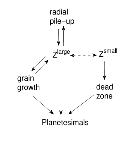
Figure 11.— Summary of logical relations between various factors relevant to planetesimal formation. A solid arrow from A to B indicates that A promotes B. Dashed double arrow indicates speculated connection between the two processes. $Z^{\rm large}$ represents metallicity for large particles (millimeter or larger), $Z^{\rm small}$ represents the abundance for micron-sized small grains. Radial pile-up denotes the pile-up of particles due to the positive radial gradient of the radial drift velocity. We refer to “Grain growth” as collisional coagulation towards the largest solid size. “Dead zone” refers to the radial extent of the dead zone. See text for details.

7.2.1 Conditions for Strong Particle Clumping

Our simulations show a dichotomy in the parameter space in which strong particle clumping occurs. Strong clumping requires the presence of relatively large particles with $\tau_{s}\gtrsim 10^{-2}$, and the abundance of these particles to be super-solar. These two requirements are represented by the two arrows connecting $Z^{\rm large}$ and “grain growth” to “planetesimals” in Figure 11. These two requirements can compensate each other: to form planetesimals, less grain growth is required if the solid abundance is large enough. In the case that all solids are strongly coupled to the gas, enhancing the disk metallicity by a factor of 5-30 may be able to trigger GI followed by planetesimal formation (Sekiya, 1998; Youdin & Shu, 2002; Chiang, 2008).

The particle size that corresponds to $\tau_{s}=10^{-2}$ depends on the disk model and distance from the central star. In the MMSN model, this stopping time corresponds to $2$cm particles at 1AU, and $2$mm or smaller particles at 5AU or beyond, according to equation (9). These particle sizes are about the maximum particle size obtained in the recent dust coagulation calculations (Zsom et al., 2010). For more massive disks, the corresponding particle size will be enlarged by a factor of $f_{g}$ in the Epstein regime. Since grain growth becomes more difficult when the particle size exceeds a millimeter, the SI scenario of planetesimal formation prefers less massive disks, or the outer part of the disk.

7.2.2 Enrichment of Local Solid Abundance

Enrichment of the local abundance of solids is possible by several effects, already briefly mentioned in §1. Here we focus on the mechanism proposed by Youdin & Shu (2002). For a particle at a fixed size (small, with $\tau_{s}<1$ at all disk radii considered), the (single-species) NSH radial drift velocity in PPDs decreases as the particle drifts inward. Therefore, radial drift causes the particles to pile-up towards the inner regions, leading to enhancement of the local abundance of solids. Depending on the time scale, the largest enhancement factor can reach $3-10$ in $10^{5}-10^{6}$ years (Youdin & Shu, 2002; Youdin & Chiang, 2004), starting in the outer disk and moving inwards. This process corresponds to the arrow pointing from “radial pile-up” to $Z^{\rm large}$ in Figure 11.

In this paper, we have shown that the radial drift velocity is reduced when local abundance of solids increases. This effect provides positive feedback to the enrichment process: particles pile up because the radial drift velocity is smaller at smaller disk radii. The enrichment of solid material at small disk radii further reduces the radial drift velocity, leading to stronger pile-ups. This effect corresponds to the arrow pointing from $Z^{\rm large}$ to “radial pile-up” in Figure 11. We see that the enrichment of the abundance of solids and the particle pile-up form a feedback loop that enhance each other. Therefore, we expect even stronger solid enrichment in the inner region of PPDs than previous calculations (Youdin & Shu, 2002; Youdin & Chiang, 2004) sufficient for SI and/or GI to form planetesimals within PPD dead zone.

7.2.3 Implications for Grain Growth

The radial drift velocity adopted in grain coagulation models (e.g., Brauer et al., 2008a; Birnstiel et al., 2010; Zsom et al., 2010) is generally taken from a single-species NSH equilibrium. However, we have shown that as particles settle to disk midplane, the radial drift velocity is reduced due to multi-species effects, and smallest particles can even drift outward rather than inward. More sophisticated modeling of grain growth is needed to incorporate the multi-species effects.

One consequence of the multi-species NSH equilibrium is that the enhancement of local abundance of solids strongly reduces the radial drift velocity, hence the particle mutual collision velocity. Because the radial drift velocity dominates the collision velocities for relatively large particles, we expect particles to grow larger in regions with large abundance of solids, due to the reduced collision velocity there. This effect is illustrated as an arrow pointing from $Z^{\rm large}$ to “grain growth” in Figure 11. In turn, grain growth form large particles from smaller ones, increasing the population of large particles, hence $Z^{\rm large}$, leading to the arrow pointing in the opposite direction. Again, these two effects form a feedback loop, promoting grain growth and enrichment of solid material.

7.2.4 Influence from Magnetic Activity

All our simulations ignore external sources of turbulence, particularly the MRI, by working in the dead zone of PPDs. Even very weak external turbulence with $\alpha\sim 10^{-4}$ may stir up the solids and maintain them at a height that may be insufficient for SI to form dense particle clumps (see Table 2). Johansen et al. (2007) showed that planetesimal formation is facilitated by MRI due to the long-lived overdensity regions that effectively trap the particles. However, they chose very large particle size with $\tau_{s}=0.25-1$. When smaller particles are used, they are diffused to a much larger height. Although SI may still be present with MRI turbulence and form elongated structures (Balsara et al., 2009), particle overdensities are small. Moreover, the mutual particle collision velocity is much higher in MRI turbulence (Carballido et al., 2008), which inhibits particle growth. Therefore, we expect the dead zone to be the more favored region for planetesimal formation, and planetesimal formation should be easier in PPDs with a larger (radial) extent of the dead zone. This is shown as the arrow pointing from “dead zone” towards “planetesimal formation” in Figure 11.

At the same time, the vertical and radial extent of the dead zone in PPDs strongly depend on the abundance of micron-sized and smaller grains (Ilgner & Nelson, 2006; Bai & Goodman, 2009), which is reflected in the arrow connecting $Z^{\rm small}$ and “dead zone”. Whether there is any connection between $Z^{\rm large}$ and $Z^{\rm small}$ is uncertain. Both $Z^{\rm large}$ and $Z^{\rm small}$ should be correlated with the overall disk metallicity. Moreover, with more large particles (larger $Z^{\rm large}$, collisional fragmentation may lead to more small grains (larger $Z^{\rm small}$). Despite many uncertainties, we draw a dashed double-arrow between $Z^{\rm large}$ and $Z^{\rm small}$ as our speculated connection between the two particle populations. If such connection exist, it represents the third way for (local) solid abundance enrichment to promote planetesimal formation.

7.3. Limitations and Outlook

Our simulations take a local patch from a simple global disk model in which all physical quantities follow a power-law dependence on disk radii. The global structure of PPDs may be more complicated. In particular, the presence of a dead zone in PPDs changes the steady-state disk surface density profile, and may lead to local pressure maxima at the snow line (Kretke & Lin, 2007; Brauer et al., 2008b), and the inner edge of the dead zone (Dzyurkevich et al., 2010). These pressure bumps are able to trap particles very efficiently. Moreover, solids can also be trapped in long-lived vortices (Barge & Sommeria, 1995; Klahr & Henning, 1997; Klahr & Bodenheimer, 2003; Johansen et al., 2004; Lyra et al., 2009), although their existence is in debate. Finally, the structure of PPDs may be very non-steady, and undergo periods of outburst (Zhu et al., 2009). Global models take into account large-scale variations of disk structure and can follow the disk evolution. Currently, the numerical resolution required for resolving the SI is prohibitively high for running 3D global simulations. Nevertheless, one can perform local simulations in different disk environments, and piece them together to form a global picture, as in Tilley et al. (2009).

Our simulations focus on the dynamics in the vicinity of the disk midplane with very limited radial and vertical box sizes and no magnetic field. This is mainly constrained by the fine grid resolution required for this study. In reality, MRI turbulence in the active layers may excite vertical oscillations in the disk midplane(Fleming & Stone, 2003; Oishi & Mac Low, 2009). Moreover, turbulent diffusion of ions may produce magnetic activity at the disk midplane, making it “undead” (Turner & Sano, 2008). Finally, turbulent mixing of particles may become important when the active layer is relatively thick (Turner et al., 2010). Including these effects into numerical simulations of planetesimal formation requires enlarging our box size in all dimensions by a factor of at least 10. Moreover, 3D rather than 2D simulations are necessary to maintain sustained MRI turbulence. Such simulations are computationally expensive, however recently the static mesh refinement (SMR) algorithm in the Athena MHD code has been parallelized. The cost of hybrid (particles and gas) simulations of layered disks can be substantially reduced by using fine resolution at the disk midplane (to capture the SI) and in the active layers (to capture the MRI), while using coarse resolution everywhere else. With SMR, it becomes feasible to study the effect of (non-ideal) MRI turbulence in the active layer on particle dynamics and planetesimal formation in the disk midplane. This is planned as future work.

Appendix A A. Multi-species NSH equilibrium

In this appendix we generalize the NSH equilibrium solution to include multi-species of particles. We start from the force balance for both gas and particle components. Their velocities are denoted by ${\boldsymbol{u}}$ for gas and ${\boldsymbol{v}}_{k}$ for particle type $k$. $\tau_{k}$ and $\epsilon_{k}$ denote dimensionless particle stopping time and solid to gas mass ratio for particle type $k$. In writing down the equations, we subtract both gas and particle velocities by linear Keplerian shear $-(3/2)\Omega x\hat{\boldsymbol{y}}$, and denote the remaining velocities by $\boldsymbol{u}^{\prime}$ and $\boldsymbol{v}^{\prime}_{k}$ respectively. Neglecting vertical gravity, the hydrostatic equilibrium equations read

$$2v^{\prime}_{ky}\hat{\boldsymbol{x}}-\frac{1}{2}v^{\prime}_{kx}\hat{\boldsymbol{y}}-\frac{1}{\tau_{k}}(\boldsymbol{v}^{\prime}_{k}-\boldsymbol{u}^{\prime})=0\ ,$$ (A1a)

$$2u^{\prime}_{y}\hat{\boldsymbol{x}}-\frac{1}{2}u^{\prime}_{x}\hat{\boldsymbol{y}}+\sum_{k}\frac{\epsilon_{k}}{\tau_{k}}(\boldsymbol{v}^{\prime}_{k}-\boldsymbol{u}^{\prime})=-2\eta v_{K}\hat{\boldsymbol{x}}\ .$$ (A1b)

Multiplying equation (A1a) by $\epsilon_{k}$ for each $k$ and adding them to equation (A1b), we find the expression of the gas velocity in terms of particle velocities

$$\boldsymbol{u}^{\prime}=-\sum_{k}\epsilon_{k}\boldsymbol{v}^{\prime}_{k}-\eta v_{K}\hat{\boldsymbol{y}}\ .$$ (A2)

To obtain the particle velocities, we define velocity vectors $\Upsilon_{x}\equiv(v^{\prime}_{1x},v^{\prime}_{2x},\ldots,v^{\prime}_{nx})^{T}$, and $\Upsilon_{y}\equiv(v^{\prime}_{1y},v^{\prime}_{2y},\ldots,v^{\prime}_{ny})^{T}$. Further we define a diagonal matrix $\Lambda\equiv{\rm diag}\{\tau_{1},\tau_{2},\ldots,\tau_{n}\}$, and a rank 1 matrix $\Gamma\equiv(\boldsymbol{\epsilon},\boldsymbol{\epsilon},\ldots,\boldsymbol{\epsilon})^{T}$, where $\boldsymbol{\epsilon}\equiv(\epsilon_{1},\epsilon_{2},\ldots,\epsilon_{n})^{T}$. With these notations, the equations governing $\boldsymbol{v}^{\prime}_{k}$ can be written as

$$\begin{pmatrix}1+\Gamma&-2\Lambda\\ \Lambda/2&1+\Gamma\end{pmatrix}\begin{pmatrix}\Upsilon_{x}\\ \Upsilon_{y}\end{pmatrix}=-\eta v_{K}\begin{pmatrix}0\\ 1\end{pmatrix}\ .$$ (A3)

The solution of this equation can not be expressed simply; but taking advantage of the block structure of the matrices, one can find the solution in the form

$$\begin{pmatrix}\Upsilon_{x}\\ \Upsilon_{y}\end{pmatrix}=-\eta v_{K}\begin{pmatrix}A&2B\\ -B/2&A\end{pmatrix}\begin{pmatrix}0\\ 1\end{pmatrix}\ ,$$ (A4)

where

$$B=\{[\Lambda^{-1}(1+\Gamma)]^{2}+1\}^{-1}\Lambda^{-1}\ ,\qquad A=\Lambda^{-1}(1+\Gamma)B\ .$$ (A5)

One can easily verify that equation (A4) indeed generalizes the single species NSH solution. The multi-species solution obtained here is useful for setting initial conditions of the simulation as well as analysis of simulation data.

Appendix B B. Collision Velocity Distribution

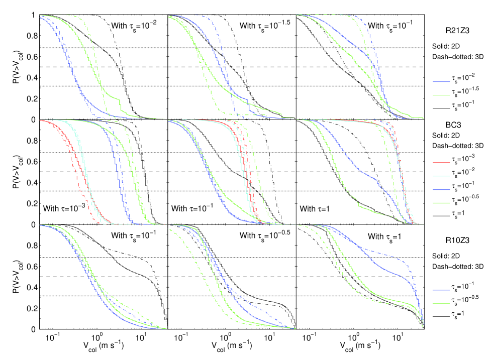
Figure 12.— The cumulative probability distribution function (CPDF) of two-body particle collision velocities from runs R21Z3 (top), R30Z3 (middle) and R10Z3 (bottom), illustrating the effect of particle clumping on collision velocities. Results from both 2D (solid) and 3D (dash-dotted) simulations are shown. In each panel, we plot the CPDFs for collisions between various particle species (with different colors, see figure legends) and one specific particle species with fixed $\tau_{s}$ (indicated in each panel). Dashed lines mark the median value, while dotted lines mark the $1\sigma$ level of fluctuations. Note that 3D runs in R21 and R30 do not show particle clumping, while the others do.

In this appendix we discuss the distribution of particle collision velocities. In Figure 12 we show the CPDFs from runs R21Z3, R30Z3 and R10Z3 (for both 2D and 3D). Each panel plots the collision velocity CPDFs between several (or all) particle species and a given particle species. The median of the collision velocity is represented by the dashed lines at $P=0.5$, with $1\sigma$ range obtained by cutting the plots at $P=0.68$ and $P=0.32$, shown in dotted lines.

Two 3D runs R21Z3-3D and R30Z3-3D do not show strong particle clumping, and their CPDFs are representative of runs without particle clumping. The CPDF curves for different pairs of particle types are very similar between each other. The curves are generally anti-symmetric with respect to the median value $P=0.5$, and the corresponding velocity distribution is close to log-normal distribution with super-exponential cutoff at large velocity. Moreover, even in runs that show strong particle clumping, the CPDFs for collisions between relatively small particles with $\tau_{s}\lesssim 10^{-2}$ also approaches the log-normal form, as one can see from run R30Z3-2D. The $1\sigma$ limit of the collision velocity is generally less than half of the median collision velocity.

The CPDFs from simulations that show strong clumping deviates substantially from log-normal. For runs R21Z3 and R30Z3, the collision velocity is clearly reduced in 2D relative to 3D (2D runs show clumping while 3D runs do not). In run R30Z3-2D, we see that the reduction is most significant for collisions between two relatively large particles with $\tau_{s}\gtrsim 0.1$, which are the ones that make up most of the clumps (see Figure 6). The collision velocity between large ($\tau_{s}>0.1$) and small ($\tau_{s}<0.1$) particles is also reduced, although to a lesser extent. For R21Z3-2D and R10Z3 (both 2D and 3D) runs, all particles actively participate in the SI and clumping, and their mutual collision velocities are all reduced. The reduction of collision velocity appears to be stronger in R30Z3 and R10Z3 runs, where $\tau_{\rm max}=1$. Finally, we see that the reduction of collision velocity is most significant for intermediate high-velocity collisions ($V_{\rm col}\simeq 1-5$m s^-1), although there is still a high-velocity tail present. It is likely that the high-velocity tail is caused by collisions outside the particle clump.

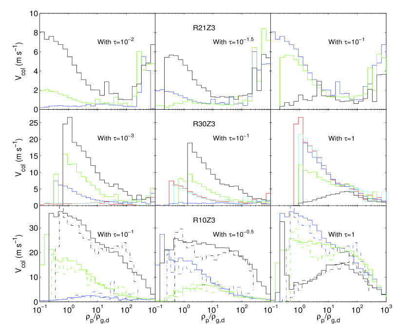
Figure 13.— The mean particle collision velocity as a function of particle density for the three runs that show particle clumping (R21Z3, R30Z3 and R10Z3, from top to bottom). The 2D results are shown in solid lines, while 3D results are shown as dash-dotted lines (bottom panels only). In each panel, we show the median collision velocity between various particle species (using the same color scheme in Figure 12) and a specific particle species with a $\tau_{s}$ as indicated in each panel.

To further address the influence of clumping on particle collision velocities, we evaluate the mean collision velocity as a function of ambient particle density $\rho_{p}$. For the three sets of runs that show particle clumping R21Z3 (2D), R30Z3 (2D) and R103 (2D and 3D), we show the results in Figure 13. For both R30Z3 and R10Z3 runs, we find a clear trend that the collision velocity is strongly reduced towards higher $\rho_{p}$. More specifically, the reduction is most prominent for collisions between large and small particles. The collision velocity between particles of similar sizes appears to be insensitive to $\rho_{p}$, and is maintained at a relatively low value. Interestingly, results from run R21Z3-2D show a different behavior. The collision velocity decreases with $\rho_{p}$ until $\rho_{p}/\rho_{g,b}\sim 300$. Beyond this density, we observe an increase of collision velocity towards larger $\rho_{p}$. We have performed an additional R41 run in 2D with Z=0.05, which shows particle clumping, and the collision velocity shows similar properties as in R21Z3-2D. This is very likely to be due to the different properties of the SI for particles with $\tau_{s}=0.1$ from particles with $\tau_{s}=1$. As shown in non-stratified simulations (Johansen & Youdin, 2007), clumps are much more dynamic in the former case, which may lead to larger collision velocities.

References

- Alexander & Armitage (2007) Alexander, R. D. & Armitage, P. J. 2007, MNRAS, 375, 500
- Bai & Goodman (2009) Bai, X.-N. & Goodman, J. 2009, ApJ, 701, 737
- Bai & Stone (2010a) Bai, X.-N. & Stone, J. 2010a, ApJS, accepted, arXiv:1005.4980
- Bai & Stone (2010b) —. 2010b, ApJL, submitted, arXiv:1005.4981
- Balbus & Hawley (1991) Balbus, S. A. & Hawley, J. F. 1991, ApJ, 376, 214
- Balsara et al. (2009) Balsara, D. S., Tilley, D. A., Rettig, T., & Brittain, S. D. 2009, MNRAS, 397, 24
- Barge & Sommeria (1995) Barge, P. & Sommeria, J. 1995, A&A, 295, L1
- Barranco (2009) Barranco, J. A. 2009, ApJ, 691, 907
- Binney & Tremaine (2008) Binney, J. & Tremaine, S. 2008, Galactic Dynamics: Second Edition, ed. Binney, J. & Tremaine, S. (Princeton University Press)
- Birnstiel et al. (2010) Birnstiel, T., Dullemond, C. P., & Brauer, F. 2010, A&A, 513, A79
- Blum & Wurm (2000) Blum, J. & Wurm, G. 2000, Icarus, 143, 138
- Blum & Wurm (2008) —. 2008, ARA&A, 46, 21
- Brauer et al. (2008a) Brauer, F., Dullemond, C. P., & Henning, T. 2008a, A&A, 480, 859
- Brauer et al. (2008b) Brauer, F., Henning, T., & Dullemond, C. P. 2008b, A&A, 487, L1
- Carballido et al. (2008) Carballido, A., Stone, J. M., & Turner, N. J. 2008, MNRAS, 386, 145
- Chandrasekhar (1961) Chandrasekhar, S. 1961, Hydrodynamic and hydromagnetic stability, ed. Chandrasekhar, S.
- Chapman & Cowling (1970) Chapman, S. & Cowling, T. G. 1970, The mathematical theory of non-uniform gases. an account of the kinetic theory of viscosity, thermal conduction and diffusion in gases (Cambridge: University Press, 1970, 3rd ed.)
- Chiang (2008) Chiang, E. 2008, ApJ, 675, 1549
- Chiang & Youdin (2009) Chiang, E. & Youdin, A. 2010, Annual Review of Earth and Planetary Sciences, 38, 493
- Chiang et al. (2001) Chiang, E. I., Joung, M. K., Creech-Eakman, M. J., Qi, C., Kessler, J. E., Blake, G. A., & van Dishoeck, E. F. 2001, ApJ, 547, 1077
- Cuzzi et al. (1993) Cuzzi, J. N., Dobrovolskis, A. R., & Champney, J. M. 1993, Icarus, 106, 102
- Cuzzi et al. (2001) Cuzzi, J. N., Hogan, R. C., Paque, J. M., & Dobrovolskis, A. R. 2001, ApJ, 546, 496
- Cuzzi et al. (2008) Cuzzi, J. N., Hogan, R. C., & Shariff, K. 2008, ApJ, 687, 1432
- D’Alessio et al. (2006) D’Alessio, P., Calvet, N., Hartmann, L., Franco-Hernández, R., & Servín, H. 2006, ApJ, 638, 314
- Dominik & Tielens (1997) Dominik, C. & Tielens, A. G. G. M. 1997, ApJ, 480, 647
- Dullemond & Dominik (2005) Dullemond, C. P. & Dominik, C. 2005, A&A, 434, 971
- Dzyurkevich et al. (2010) Dzyurkevich, N., Flock, M., Turner, N. J., Klahr, H., & Henning, T. 2010, ArXiv e-prints
- Epstein (1924) Epstein, P. S. 1924, Phys. Rev., 23, 710
- Fleming & Stone (2003) Fleming, T. & Stone, J. M. 2003, ApJ, 585, 908
- Fromang & Nelson (2005) Fromang, S. & Nelson, R. P. 2005, MNRAS, 364, L81
- Fromang & Nelson (2009) —. 2009, A&A, 496, 597
- Gammie (1996) Gammie, C. F. 1996, ApJ, 457, 355
- Garaud & Lin (2004) Garaud, P. & Lin, D. N. C. 2004, ApJ, 608, 1050
- Goldreich et al. (2004) Goldreich, P., Lithwick, Y., & Sari, R. 2004, ARA&A, 42, 549
- Goldreich & Lynden-Bell (1965) Goldreich, P. & Lynden-Bell, D. 1965, MNRAS, 130, 125
- Goldreich & Ward (1973) Goldreich, P. & Ward, W. R. 1973, ApJ, 183, 1051
- Gómez & Ostriker (2005) Gómez, G. C. & Ostriker, E. C. 2005, ApJ, 630, 1093
- Goodman & Pindor (2000) Goodman, J. & Pindor, B. 2000, Icarus, 148, 537
- Güttler et al. (2009) Güttler, C., Blum, J., Zsom, A., Ormel, C. W., & Dullemond, C. P. 2010, A&A, 513, A56
- Hartmann et al. (1998) Hartmann, L., Calvet, N., Gullbring, E., & D’Alessio, P. 1998, ApJ, 495, 385
- Hawley & Balbus (1991) Hawley, J. F. & Balbus, S. A. 1991, ApJ, 376, 223
- Hawley et al. (1995) Hawley, J. F., Gammie, C. F., & Balbus, S. A. 1995, ApJ, 440, 742
- Hayashi (1981) Hayashi, C. 1981, Progress of Theoretical Physics Supplement, 70, 35
- Ida & Lin (2004a) Ida, S. & Lin, D. N. C. 2004a, ApJ, 604, 388
- Ida & Lin (2004b) —. 2004b, ApJ, 616, 567
- Ilgner & Nelson (2006) Ilgner, M. & Nelson, R. P. 2006, A&A, 445, 205
- Johansen et al. (2004) Johansen, A., Andersen, A. C., & Brandenburg, A. 2004, A&A, 417, 361
- Johansen et al. (2006a) Johansen, A., Henning, T., & Klahr, H. 2006a, ApJ, 643, 1219
- Johansen et al. (2006b) Johansen, A., Klahr, H., & Henning, T. 2006b, ApJ, 636, 1121
- Johansen et al. (2007) Johansen, A., Oishi, J. S., Low, M.-M. M., Klahr, H., Henning, T., & Youdin, A. 2007, Nature, 448, 1022
- Johansen & Youdin (2007) Johansen, A. & Youdin, A. 2007, ApJ, 662, 627
- Johansen et al. (2009) Johansen, A., Youdin, A., & Mac Low, M. 2009, ApJ, 704, L75
- Kenyon & Bromley (2006) Kenyon, S. J. & Bromley, B. C. 2006, AJ, 131, 1837
- Klahr & Bodenheimer (2003) Klahr, H. H. & Bodenheimer, P. 2003, ApJ, 582, 869
- Klahr & Henning (1997) Klahr, H. H. & Henning, T. 1997, Icarus, 128, 213
- Kokubo & Ida (1998) Kokubo, E. & Ida, S. 1998, Icarus, 131, 171
- Kretke & Lin (2007) Kretke, K. A. & Lin, D. N. C. 2007, ApJ, 664, L55
- Lee et al. (2010a) Lee, A. T., Chiang, E., Asay-Davis, X., & Barranco, J. A. 2010a, ApJ, 718, 1367
- Lee et al. (2010b) Lee, A. T., Chiang, E., Asay-Davis, X., & Barranco, J. A. 2010b, ApJ, submitted
- Lissauer & Stewart (1993) Lissauer, J. J. & Stewart, G. R. 1993, in Protostars and Planets III, ed. E. H. Levy & J. I. Lunine, 1061–1088
- Lodders (2003) Lodders, K. 2003, ApJ, 591, 1220
- Lyra et al. (2009) Lyra, W., Johansen, A., Zsom, A., Klahr, H., & Piskunov, N. 2009, A&A, 497, 869
- Markiewicz et al. (1991) Markiewicz, W. J., Mizuno, H., & Voelk, H. J. 1991, A&A, 242, 286
- Michikoshi et al. (2010) Michikoshi, S., Kokubo, E., & Inutsuka, S. 2010, ApJ, 719, 1021
- Morbidelli et al. (2009) Morbidelli, A., Bottke, W. F., Nesvorný, D., & Levison, H. F. 2009, Icarus, 204, 558
- Nakagawa et al. (1986) Nakagawa, Y., Sekiya, M., & Hayashi, C. 1986, Icarus, 67, 375
- Oishi & Mac Low (2009) Oishi, J. S. & Mac Low, M. 2009, ApJ, 704, 1239
- Ormel & Cuzzi (2007) Ormel, C. W. & Cuzzi, J. N. 2007, A&A, 466, 413
- Pollack et al. (1996) Pollack, J. B., Hubickyj, O., Bodenheimer, P., Lissauer, J. J., Podolak, M., & Greenzweig, Y. 1996, Icarus, 124, 62
- Safronov (1969) Safronov, V. S. 1969, Evolution of the protoplanetary cloud and formation of the earth and the planets (Moscow: Nauka Press. Trans. NASA TTF 677, 1972)
- Salmeron & Wardle (2008) Salmeron, R. & Wardle, M. 2008, MNRAS, 388, 1223
- Sano et al. (2000) Sano, T., Miyama, S. M., Umebayashi, T., & Nakano, T. 2000, ApJ, 543, 486
- Sekiya (1998) Sekiya, M. 1998, Icarus, 133, 298
- Stone & Gardiner (2010) Stone, J. M. & Gardiner, T. A. 2010, ApJS, 189, 142
- Stone et al. (2008) Stone, J. M., Gardiner, T. A., Teuben, P., Hawley, J. F., & Simon, J. B. 2008, ApJS, 178, 137
- Stone et al. (1996) Stone, J. M., Hawley, J. F., Gammie, C. F., & Balbus, S. A. 1996, ApJ, 463, 656
- Testi et al. (2003) Testi, L., Natta, A., Shepherd, D. S., & Wilner, D. J. 2003, A&A, 403, 323
- Throop & Bally (2005) Throop, H. B. & Bally, J. 2005, ApJ, 623, L149
- Tilley et al. (2009) Tilley, D. A., Balsara, D. S., Brittain, S. D., & Rettig, T. 2010, MNRAS, 403, 211
- Turner et al. (2010) Turner, N. J., Carballido, A., & Sano, T. 2010, ApJ, 708, 188
- Turner & Drake (2009) Turner, N. J. & Drake, J. F. 2009, ApJ, 703, 2152
- Turner & Sano (2008) Turner, N. J. & Sano, T. 2008, ApJ, 679, L131
- Voelk et al. (1980) Voelk, H. J., Jones, F. C., Morfill, G. E., & Roeser, S. 1980, A&A, 85, 316
- Weidenschilling (1977) Weidenschilling, S. J. 1977, MNRAS, 180, 57
- Weidenschilling (1980) —. 1980, Icarus, 44, 172
- Wetherill & Stewart (1989) Wetherill, G. W. & Stewart, G. R. 1989, Icarus, 77, 330
- Youdin & Johansen (2007) Youdin, A. & Johansen, A. 2007, ApJ, 662, 613
- Youdin (2005a) Youdin, A. N. 2005a, arXiv:astro-ph/0508659
- Youdin (2005b) —. 2005b, arXiv:astro-ph/0508662
- Youdin & Chiang (2004) Youdin, A. N. & Chiang, E. I. 2004, ApJ, 601, 1109
- Youdin & Goodman (2005) Youdin, A. N. & Goodman, J. 2005, ApJ, 620, 459
- Youdin & Lithwick (2007) Youdin, A. N. & Lithwick, Y. 2007, Icarus, 192, 588
- Youdin & Shu (2002) Youdin, A. N. & Shu, F. H. 2002, ApJ, 580, 494
- Zhu et al. (2009) Zhu, Z., Hartmann, L., & Gammie, C. 2009, ApJ, 694, 1045
- Zsom et al. (2010) Zsom, A., Ormel, C. W., Guettler, C., Blum, J., & Dullemond, C. P. 2010, A&A, 513, A57