The Bolocam Galactic Plane Survey – III. Characterizing Physical Properties of Massive Star-Forming Regions in the Gemini OB1 Molecular Cloud

Abstract

We present the 1.1 millimeter Bolocam Galactic Plane Survey (BGPS) observations of the Gemini OB1 molecular cloud complex, and targeted NH₃ observations of the BGPS sources. When paired with molecular spectroscopy of a dense gas tracer, millimeter observations yield physical properties such as masses, radii, mean densities, kinetic temperatures and line widths. We detect 34 distinct BGPS sources above 5$\sigma=0.37$ Jy beam^-1 with corresponding 5$\sigma$ detections in the NH₃(1,1) transition. Eight of the objects show water maser emission (20%). We find a mean millimeter source FWHM of 1.12 pc, and a mean gas kinetic temperature of 20 K for the sample of 34 BGPS sources with detections in the NH₃(1,1) line. The observed NH₃ line widths are dominated by non-thermal motions, typically found to be a few times the thermal sound speed expected for the derived kinetic temperature. We calculate the mass for each source from the millimeter flux assuming the sources are isothermal and find a mean isothermal mass within a 120″ aperture of $230\pm 180$ M_⊙. We find a total mass of 8,400 M_⊙ for all BGPS sources in the Gemini OB1 molecular cloud, representing 6.5% of the cloud mass. By comparing the millimeter isothermal mass to the virial mass within a radius equal to the mm source size calculated from the NH₃ line widths, we find a mean virial parameter ($M_{vir}$/$M_{iso}$) of 1.0$\pm$0.9 for the sample. We find mean values for the distributions of column densities of $1.0\times 10^{22}$ cm^-2 for H₂, and $3.0\times 10^{14}$ cm^-2 for NH₃, giving a mean NH₃ abundance of $3.0\times 10^{-8}$ relative to H₂. We find volume-averaged densities on the order of $10^{3}-10^{4}$ cm^-3. The sizes and densities suggest that in the Gem OB 1 region the BGPS is detecting the clumps from which stellar clusters form, rather than smaller, higher density cores where single stars or small multiple systems form.

1. Introduction

The availability of millimeter bolometer arrays has made possible large-scale, blind surveys of the cold dust most closely associated with star formation (e.g., Enoch et al. 2007; Motte et al. 2007; Aguirre et al. 2010; Schuller et al. 2009). Such blind millimeter continuum surveys can identify the clumps where massive stars and clusters are born without the requirement of a signpost of massive star formation, such as maser emission (e.g., Palla et al. 1991; Plume et al. 1992; Plume et al. 1997; Beuther et al 2002; Mueller et al. 2002; Shirley et al. 2003), radio continuum emission (e.g., Ramesh & Sridharan 1997; Sridharan 2002), infrared sources (e.g., Molinari et al 2000; Kumar et al. 2006; Kumar & Grave 2007; Robitaille et al 2008), or infrared colors (Wood & Churchwell 1989). Infrared dark clouds (IRDCs; regions of high density seen in absorption against the diffuse mid-IR background which are thought to represent the earliest stages of massive star formation) provide another way to find regions of massive star formation (Rathborne et al. 2006; Jackson et al. 2008), but only if they lie in front of extended mid-IR emission. However, IRDCs are seen in emission at mm wavelengths, allowing the BGPS to detect the earliest stages of massive star formation at larger distances where a significant mid-IR background is absent or too much foreground mid-IR emission is present.

Galaxy-wide millimeter continuum surveys, in conjunction with distance information, will allow us to determine the physical properties of a vast number of sources and begin answering some important questions. What is the impact of environment on star formation? How do the physical properties of clumps, such as size, mass, and mean density vary as a function of Galactocentric radius and proximity to a spiral arm? Answering these questions will provide a greater understanding of star formation in our own Galaxy. Also, by characterizing the distribution of dense gas clumps in our own galaxy, we can better understand the aggregate emission of clumps in distant galaxies where the dense gas structures cannot be resolved.

In this paper, we refer to clumps as distinct bound regions within molecular clouds that will form entire stellar clusters, and cores as the regions within clumps that will form a single star or small multiple system (e.g., Williams et al. 2000). Clumps can be characterized with masses ranging from $50-500$ M_⊙, sizes ranging from $0.3-3$ pc, mean densities ranging from $10^{3}-10^{4}$ cm^-3, and gas temperatures ranging from $10-20$ K, while starless cores can be characterized by masses from $0.5-5$ M_⊙, sizes of $0.03-0.2$ pc, mean densities of $10^{4}-10^{5}$ cm^-3, and gas temperatures between 8 and 12 K (Bergin & Tafalla 2007).

The Bolocam Galactic Plane Survey (BGPS) is one of the first millimeter surveys of the northern Galactic plane (Aguirre et al. 2009), and has cataloged 8,358 sources (Rosolowsky et al. 2009). The BGPS consists of two parts: a blind survey of the inner Galaxy, and a targeted survey of well-known star-forming regions in the outer Galaxy. The inner Galaxy survey coverage is continuous over $-10\mbox{${}^{\circ}$}<l<90.5\mbox{${}^{\circ}$}$, and the outer Galaxy coverage includes IC1396, the W3/4/5 region, 4 square degrees towards the Perseus Arm (near NGC 7538), and the Gemini OB1 molecular cloud. With a large range in Galactic longitude, the BGPS provides the opportunity to study star formation in drastically different environments.

Millimeter continuum emission detected in the BGPS can arise from all objects along a line of sight, from a few hundred pc to the other side of the Galaxy; distances to BGPS sources are not known a priori. With recent improvements to kinematic models of the Galaxy (e.g., Pohl et al. 2008) and VLBI parallax distances (Reid et al. 2009), radial velocities can yield kinematic distances. Molecular spectral lines also provide information regarding the kinematics within each source. Ammonia (NH₃), in particular, is an excellent tracer of dense gas which also provides information regarding the line of sight velocity dispersion, kinetic gas temperature, column density and mass (e.g., Ho & Townes 1983; Zinchenko et al. 1997; Swift et al. 2005; Rosolowsky et al. 2008; Foster et al. 2009). Pairing the 1.1 mm continuum data with NH₃ observations allows complete characterization of both the gas and dust properties (e.g., Rosolowsky et al. 2008; Foster et al. 2009).

In this paper, we present the results of an NH₃ survey of the BGPS sources in the Gemini OB1 molecular cloud. In §2 we provide an overview of the structure and previous observations of the Gemini OB1 molecular cloud. We briefly describe the BGPS and NH₃ surveys and data reduction in §3, and present the parameter estimation methods in §4. In §5 we discuss the basic results of the BGPS and NH₃ in the Gemini OB1 molecular cloud, and in §6 we discuss the derived physical properties in detail. We compare our results to previous studies in §7.1, and explore the effects of distance on the derived properties in §7.2. Finally, we present a summary in §8. In future work, we will present GBT+BGPS observations of sources at low Galactic longitudes.

Studying the Gem OB1 region is particularly useful because the BGPS sources in this region are located in the same molecular complex and thus have similar distances (Carpenter et al. 1995a; Carpenter et al. 1995b). We are able to investigate the physical properties of this subset of BGPS sources without the ambiguity introduced by a large range of distances seen for the sample as a whole. This paper will serve as a Galactic anti-center comparison for a study of NH₃ observations of BGPS sources at a range of Galactic longitudes in the inner Galaxy (M. K. Dunham et al., in prep.).

2. Gemini OB1 Molecular Cloud

Gemini OB1 is an OB association centered near $(l,b)=(189$^∘$,1$^∘$)$ which was first identified by Morgan, Whitford, & Code (1953). It became known as Gem OB1 when Humphreys (1978) compiled a list of the brightest OB stars in the Milky Way, cataloging 20 OB stars as belonging to the association. Many groups have studied the association and found distances ranging from 1.4 kpc to 1.9 kpc (Crawford et al. 1955; Hardie et al. 1960; Georgelin et al. 1973; Humphreys 1978). There is also a significant spread in age amongst the association members, with ages ranging from 2 Myr (Grasdalen & Carrasco 1975) to 10 Myr (Barbaro et al. 1969).

The Gemini OB1 molecular cloud was first identified as an enhancement of emission in the Columbia ¹²CO survey of the Galactic plane (Dame et al. 1987), and spans a $6\mbox{${}^{\circ}$}\times 6\mbox{${}^{\circ}$}$ area on the sky (Huang & Thaddeus 1986). There are many star-forming regions in the Gem OB1 molecular cloud, including well-known HII regions S247, S252, the group S254, S255, S256, S257, and S258 (hereafter referred to as S254-258), S259, S261 (Sharpless 1959), and BFS 52 as well as a supernova remnant, IC 443. Reid et al. (2009) used the VLBA to measure the parallax of methanol masers in S252, and found a distance of $2.10\pm 0.026$ kpc, which we adopt in this study.

Studies of ¹²CO and ¹³CO in the Gem OB1 molecular cloud show abundant arc and ring-like filamentary structure (Carpenter et al. 1995a; Kömpe et al. 1989). Carpenter et al. (1995a) mapped 32 square degrees of the Gem OB1 molecular cloud in ¹²CO($J=1-0$) and ¹³CO($J=1-0$) with 50″ sampling and 45″ and 50″ resolution respectively. They suggest that the filamentary structure is comprised of molecular material which has been swept-up by the expanding HII regions and wind blown bubbles. They conclude that the high column density regions where star formation is currently occurring were formed through the interaction of newly formed stars and the surrounding molecular material. Carpenter et al. (1995a) split the cloud into 7 separate regions and find that 3 regions (S247, S252, and S254-258) contain active star formation based on higher H₂ column densities ($>10^{22}$ cm^-2) and warmer kinetic temperatures (10 to 30 K).

Carpenter et al. (1995b) identified 11 clumps within the ¹²CO filaments using CS($J=2-1$) observations (55″ resolution), all with masses greater than 100 M_⊙. They found that at least eight of the 11 clumps have associated IRAS point sources. Carpenter et al. (1995b) also conducted a near-infrared imaging survey of a $30\mbox{\arcmin}\times 45\mbox{\arcmin}$ area surrounding S247, including three of the CS clumps. They found that each of the three clumps contains a cluster of stars in the near-infrared images.

Chavarría et al. (2008) identified 510 young stellar objects (YSOs) with near or mid-IR excess in the S254-258 complex using a combination of Spitzer IRAC and near-infrared data. They classify 87 Class I sources, and 165 Class II sources, and find that 80% of the YSOs are in clusters surrounded by a more evenly distributed population.

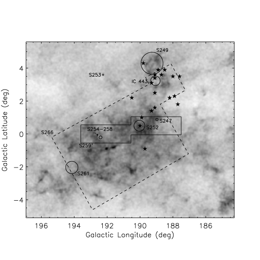
Figure 1.— The Gemini OB1 molecular cloud. Extinction maps of Dobashi et al. (2005) are shown in inverted grayscale ranging from -0.5 to 4.0 magnitudes. The OB association members (Humphreys 1978) are shown as stars. The HII regions (Sharpless 1959) and IC 443 are shown as circles sized to match the extent of the region. The dashed line marks the area mapped in ¹²CO and ¹³CO by Carpenter et al. (1995a), and the solid line marks the extent of the 1.1 mm BGPS maps.

Figure 1 shows the extinction maps of Dobashi et al. (2005) for the Gemini OB1 molecular cloud. OB association members are shown as stars (Humphreys 1978), HII regions (Sharpless 1959) and IC 443 are shown as circles with sizes corresponding to the source size. The extent of the ¹²CO and ¹³CO maps of Carpenter et al. (1995a) is marked by the dashed line, while the solid line shows the extent of the BGPS map presented in this paper.

3. Surveys

3.1. Bolocam 1.1 mm Galactic Plane Survey

The BGPS has surveyed approximately 170 square degrees of the Galactic Plane using the Bolocam instrument on the Caltech Submillimeter Observatory (CSO) on Mauna Kea. Aguirre et al. (2010) present specific details regarding the BGPS and methods and Rosolowsky et al. (2010) detail the BGPS catalog. The images and catalog have been made public and are hosted by the Infrared Processing and Analysis Center via the NASA/IPAC Infrared Science Archive (IPAC).

3.1.1 Observations

The Gem OB1 region was observed in two 3${}^{\circ}\times$1^∘ groups of observations, centered at $(l,b)=(189\mbox{${}^{\circ}$},0.5\mbox{${}^{\circ}$})$ and $(192\mbox{${}^{\circ}$},0\mbox{${}^{\circ}$})$, with a shallow observation centered between the two main groups to aid in mosaicing the images (see Figure 2). The centers were selected to place the most active star-forming regions (S247, S252, and S254-258) within our mapped region. Observations were carried out at the Caltech Submillimeter Observatory (CSO) as part of the BGPS between 9 and 13 September 2007. The survey used the Bolocam instrument, which has a hexagonal array of 144 bolometers. The Bolocam filter is centered at 268 GHz with a bandwidth of 45 GHz, and was designed to exclude the ¹²CO(2 $\rightarrow$ 1) emission line. Each bolometer beam is well approximated by a Gaussian with a FWHM of 31″, and the bolometer separation results in an instantaneous field of view of 7.5′. For the BGPS, the effective beam size after processing many scans is 33″ for the current release (Aguirre et al. 2010). For more instrument specific details, see Glenn et al. (2003) and Haig et al. (2004). Observations were obtained using the raster scan mode, with alternating scans directed along $l$ and $b$. The scan speed was 120″ s^-1, and chopping was not utilized in these observations, thereby retaining some sensitivity to large scale structure up to the angular size of the array (see Aguirre et al. 2010 for more detailed analysis).

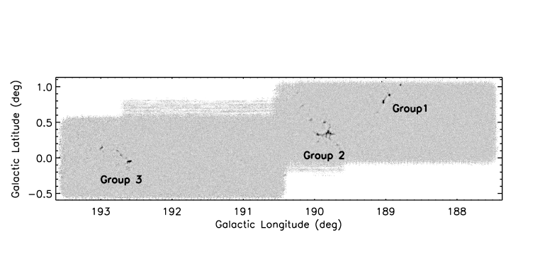
Figure 2.— The BGPS 1.1 mm continuum image of the Gemini OB1 molecular cloud shown in an inverted, linear grayscale ranging from -0.2 to 0.75 Jy beam^-1. Groups 1, 2, and 3 are shown in more detail in following figures.

3.1.2 Reduction

At millimeter wavelengths, the detected signal is dominated by the atmosphere, making the sky cleaning algorithm extremely important. Bolocam’s individual bolometer beams overlap substantially in the lower atmosphere such that they probe similar columns of atmosphere, facilitating sky subtraction. The iterative mapping method utilizes principal component analysis (PCA) and considers all observations for a given field simultaneously. In our iterative mapping method, the temporally correlated signal is first subtracted from the time streams. This subtraction removes both the atmosphere and all astrophysical structure larger than the array field of view. The remaining time stream, which in principle should contain only astrophysical signal, is then mapped with 7.2″$\times$7.2″ pixels, deconvolved from the beam, and returned to a time stream. The time stream containing only astrophysical signal is subtracted from the original to produce a third time stream (summing the subtracted astrophysical signals to make a source map) that represents an estimate of the noise. The above procedure is then repeated for 50 iterations on the deconvolved astrophysical signal time stream to produce the final map. This procedure can be fine-tuned to balance the retention of large-scale structure against production of artifacts (such as negative bowls) around bright sources. The iterative mapping method resulted in a 1-$\sigma$ RMS noise of 0.070 Jy/beam in the Gemini OB1 image. For more specific information on the BGPS reduction, see Aguirre et al. (2010).

3.1.3 Images

The iteratively mapped BGPS image is shown in Figure 2. The millimeter sources in our maps are highly clustered and are found in three groups, while the remainder of the image is strikingly devoid of millimeter emission. This clustering is in contrast to the inner Galaxy regions also included in the BGPS, where a similarly sized image would contain hundreds of sources [see Aguirre et al. (2010) and J. Bally et al. (2010)]. The three groups correspond to S247 (referred to as Group 1; Figure 3), S252 (referred to as Group 2; Figure 4), and S254$-$258 (referred to as Group 3; Figure 5).

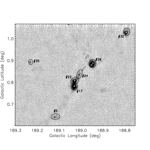
Figure 3.— The BGPS image of the region marked Group 1 in Figure 2 in inverted grayscale ranging from -0.2 to 0.75 Jy beam^-1. The BGPS sources with NH₃ spectra are shown as black ellipses, while BGPS sources without NH₃ spectra are shown as white ellipses. The NH₃ pointings are shown as crosses and diamonds. Crosses denote pointings closest to the peak of the millimeter emission, while diamonds denote additional NH₃ pointings within each BGPS source.

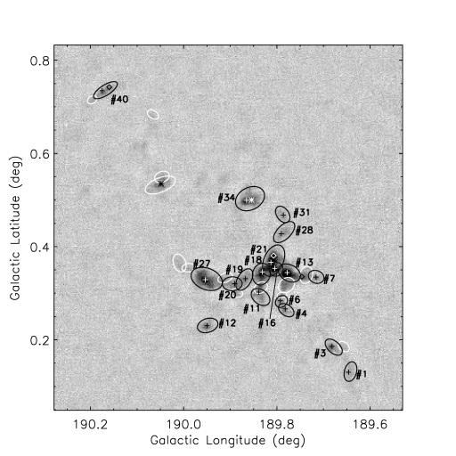
Figure 4.— The BGPS image of the region marked Group 2 in Figure 2 in inverted grayscale ranging from -0.2 to 0.75 Jy beam^-1. The BGPS sources with NH₃ spectra are shown as black ellipses, while BGPS sources without NH₃ spectra are shown as white ellipses. The NH₃ pointings are shown as crosses, diamonds and asterisks. Crosses denote pointings closest to the peak of the millimeter emission, diamonds denote additional NH₃ pointings within each BGPS source, and asterisks denote non-detections. Source ellipses can overlap since these are the moment approximations to source sizes rather than the boundaries established by the extraction algorithm.

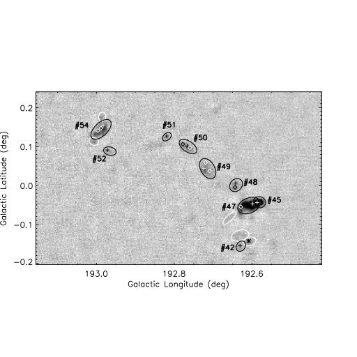
Figure 5.— The BGPS image of the region marked Group 3 in Figure 2 in inverted grayscale ranging from -0.2 to 0.75 Jy beam^-1. The BGPS sources with NH₃ spectra are shown as black ellipses, while BGPS sources without NH₃ spectra are shown as white ellipses. The NH₃ pointings are shown as crosses, diamonds and asterisks. Crosses denote pointings closest to the peak of the millimeter emission, diamonds denote additional NH₃ pointings within each BGPS source, and asterisks denote non-detections. Source ellipses can overlap since these are the moment approximations to source sizes rather than the boundaries established by the extraction algorithm.

3.2. NH₃ Survey of BGPS Sources

The NH₃ pointings are displayed in Figures 3$-$5 as crosses, diamonds, and asterisks. Since the NH₃ pointings were chosen prior to completion of the BGPS catalog, they do not necessarily correspond to the peak positions of the millimeter emission determined by the source extraction algorithm (see §4.1). Crosses mark the positions closest to the peak of the millimeter emission, diamonds mark extra NH₃ pointings within each source, and the asterisks mark the positions of NH₃ pointings which correspond to a mm source but do not have a detection in any of the NH₃ transitions.

3.2.1 Observations

We observed 56 NH₃ pointings in the Gem OB1 region using the Robert F. Byrd Green Bank Telescope (GBT) on 14 and 15 February 2008 in two separate blocks totaling 3.6 hours. The 23 GHz zenith opacity for the Feb. 14 observations was $\tau_{23}\sim 0.04$; and for Feb. 15, $\tau_{23}\sim 0.11$. The observations were broken into two minute integrations of individual targets. We used Feed 1 of the high-frequency K-band receiver on the GBT as the front end for the observations. The GBT spectrometer served as the back end, which we configured to observe both polarizations of the feed with 50 MHz bandwidth for four separate IFs. The total bandwidth was sampled in 8192 channels for a 6.1 kHz ($\sim$0.08 km s^-1) channel width. We used two different sets of IFs. All scans contained the NH₃(1,1) (23.6944955(1) GHz) and NH₃(2,2) (23.7226333(1) GHz) lines. Observations on February 14 (10 pointings) also included the C₂S (N${}_{J}=2_{1}\to 1_{0}$, 22.344033(1) GHz, Yamamoto et al. 1990) and NH₃(4,4) (24.1394169(1) GHz) lines. All NH₃ frequencies were taken from Lovas & Dragoset (2003). There were no significant detections of the C₂S line and only one marginal detection of the NH₃(4,4) line, so the spectrometer configuration was changed for the following days’ observations. The observations on February 15 included the H₂O (22.344033 GHz), and NH₃(3,3) (23.8701279(5) GHz) transitions in the remaining two IFs. Ten pointings were observed on 14 February 2008 with C₂S and NH₃(4,4), and all 56 pointings were observed with H₂O and NH₃(1,1), (2,2) and (3,3). Ten pointings were observed in all six lines (four NH₃ lines, H₂O, and C₂S). We observed each source with a symmetric, in-band frequency switch (5 MHz throw).

Observations of the Gem OB1 region were conducted immediately following observations for a pointing model correction on each night. We calibrated the data with the injection of a noise signal periodically throughout the observations. Because of slow variations in the power output of the noise diodes and their coupling to the signal path, we measured the strength of the noise signal through observations of a source with known flux (the NRAO flux calibrator 3C 48, $S_{\nu}=1.13$ Jy). We repeated the flux calibration observations during every observing session to detect any changes in the calibration sources, finding no significant variations over the course of our run ($<10\%$). The beam size of the GBT is 31″ at these frequencies, which projects to a size of 0.32 pc at the distance of Gem OB1 (2.10 kpc, see §6.1; Reid et al. (2009)). The GBT NH₃ observations are well matched to the BGPS observations since the GBT beam size is only a few arcseconds smaller than the effective BGPS beam size.

3.2.2 Data Reduction

The ammonia observations were reduced using the GBTIDL reduction package. We extracted each scan, using the package to fold the spectrum to remove the effects of the frequency switching and establish the data on the $T_{A}$ scale by calibrating the noise diodes. We subtracted a linear baseline from the spectrum from each IF with the exception of the IF containing the water and C₂S lines where a second order baseline was required. We then scaled to the $T_{A}^{*}$ scale using estimates of the atmospheric opacity interpolated in the frequency and time domains at 22 and 23 GHz from models of the atmosphere derived using weather data. To reach the $T_{mb}$ scale, the spectra are divided by the main beam efficiency of the GBT, which is $\eta_{mb}\sim 0.81$ at these frequencies. We averaged together both polarizations; if a source was observed multiple times, each observation was calibrated separately and the resulting spectra were then averaged together. The mean and standard deviation of the RMS noise per channel for each of the 6 observed lines are listed in Table 1.

Table 1Mean RMS for Spectral Line Observations

	mean RMS	stdev RMS
Line	(mK)	(mK)
NH3(1,1)	82	21
NH3(2,2)	81	21
NH3(3,3)	97	11
NH3(4,4)	52	1
H2O	172	26
C2S	67	4

4. Parameter Estimation

4.1. BGPS Parameter Estimation

The BGPS millimeter source properties are extracted from the iterative maps using the BGPS source extraction software, Bolocat (Rosolowsky et al. 2009). Bolocat utilizes a seeded watershed method (also referred to as marker-controlled segmentation; Soille 1999) which is comprised of two main steps. First, regions with emission above a signal-to-noise ratio of 2.5 are identified and expanded through a nearest-neighbor algorithm to include adjacent, lower signal-to-noise pixels. Second, each identified region is subdivided into further substructures based on the contrast between local maxima. Bolocat then determines source properties from emission-weighted moments. Two sets of coordinates are determined for each source: peak and centroid coordinates. The peak coordinates correspond to the peak of the 1.1 mm emission and are determined from median smoothed maps. The centroid coordinates are given by the first emission-weighted moments. The major and minor axis dispersions ($\sigma_{maj}$ and $\sigma_{min}$) are given by the second moments. The object radius (R_obj) is calculated from

$$R_{obj}=\eta[(\sigma_{maj}^{2}-\sigma_{beam}^{2})(\sigma_{min}^{2}-\sigma_{beam}^{2})]^{1/4},$$ (1)

where $\sigma_{beam}=\Theta_{FWHM}/\sqrt{8\ln 2}$ and $\eta$ is a factor relating the axis dispersions to the true size of the source, found to be 2.4. The value $\eta=2.4$ is adopted as the median value derived from measuring the observed axis dispersions compared with the true radius for a variety of simulated emission profiles spanning a range of density distributions, sizes relative to the beam and signal-to-noise ratios. The ellipses in Figures 3$-$5 mark the positions and sizes of the extracted BGPS sources. White ellipses denote BGPS sources which do not contain any NH₃ pointings or only contain a pointing which was not detected, and black ellipses denote BGPS sources which contain at least one detected NH₃ pointing.

Table 2Aperture Flux Corrections

Aperture
(′′)	$S_{\nu}$(int)/$S_{\nu}$(ap)
40	1.46
80	1.04
120	1.01

Source flux densities are determined by aperture photometry within standard apertures, 40″, 80″, 120″, and $2R_{obj}$ diameter apertures denoted as $S_{\nu}$(40″), $S_{\nu}$(80″), $S_{\nu}$(120″), and $S_{\nu}$(obj). An integrated flux density, $S_{\nu}$(int), is also reported for each source and is the sum of all pixels assigned to a given source by the source extraction algorithm divided by the number of pixels per beam. The intensity in the BGPS maps was calibrated based on the observed properties of planets. Aguirre et al. (2010) have compared the BGPS data to other mm continuum surveys and found that we must multiply our flux densities by 1.5$\pm$0.15 in order for our flux densities to agree with the other surveys (see Aguirre et al. (2010) for more details). In this paper we apply the flux calibration correction of 1.5$\pm$0.15 to the v1.0 BGPS products presented in Rosolowsky et al. (2010) and released on the IPAC website. All data products and properties presented in this paper include this flux calibration factor.

Aperture corrections must be applied to the photometry in order to account for power at large radii due to the non-gaussian side lobes of the CSO beam. The aperture corrections were determined by comparing the integrated flux density for known point sources to the calculated aperture flux densities. The aperture correction values are listed in Table 2. As can be seen from the aperture corrections, the 40″ aperture underestimates the flux density by almost 50%. The 80″ aperture only underestimates the flux density by approximately 4%, and the 120″ aperture requires only a 1% correction. The apertures corresponding to $2R_{obj}$ require varying aperture corrections, while $S_{\nu}$(int) represents all flux in the 1.1 mm maps down to the 1$\sigma$ level and does not require an aperture correction factor. The aperture corrections were determined based on sources very small compared to the BGPS beam and therefore will slightly overestimate the flux densities of sources which are extended compared to the beam size. For more details regarding source extraction and parameter estimation, see Rosolowsky et al. (2010).

4.2. NH₃ Parameter Estimation

We estimate physical properties of the molecular gas by fitting a simple model to each calibrated spectrum, following the method described in Rosolowsky et al. (2008; hereafter R08). The model estimates the ammonia emission that would be observed from a slab of molecular gas with a fixed optical depth in the NH₃(1,1) line of $\tau$, LSR velocity $v_{\mathrm{LSR}}$, velocity dispersion $\sigma_{v}$, radiative excitation temperature $T_{ex}$, and kinetic temperature $T_{K}$. For clarity, we note that $\tau$ here represents the total opacity in the (1,1) transition which is then apportioned into the 18 hyperfine components of the line according to their statistical weights. The central cluster of ammonia hyperfine components, which is commonly studied in isolation, contains half the total optical depth, $\tau_{main}=0.5\tau$.

The model spectrum provides a simultaneous estimate of all the ammonia parameters; however, specific aspects of the spectral data control each derived quantity. For example, the ratio of strengths of the (1,1) and (2,2) lines yields an estimate of the kinetic temperature. The model accounts for the line widths by assuming a Gaussian velocity distribution in the underlying slab of material so that the model spectrum accounts for line broadening by hyperfine structure and optical depth effects. The difference between the line strength on the $T_{mb}$ scale and the kinetic temperature provides information on the radiative excitation of the line $T_{ex}$ under the assumption that the emission fills the telescope beam (see §6.6 for more details). As noted in R08, the parameters $T_{ex}$ and $\tau$ are strongly covariant and cannot be determined separately in the low optical depth limit. In these cases, only the product $\tau T_{ex}$ is determined. At higher optical depths, the relative strengths of the central and satellite hyperfine transitions in the (1,1) line provide an independent estimate of the optical depth.

Using these parameters as a description of the underlying molecular gas, a model spectrum can be generated that adequately describes emission we observe from the Gem OB1 sources including the hyperfine structure of the ammonia transitions. The best-fit set of parameters is determined by a least-squares optimization of the model spectrum to fit to all observed ammonia transitions simultaneously. The primary advantage of this approach is the straight-forward estimation of errors and covariances in the fit parameters.

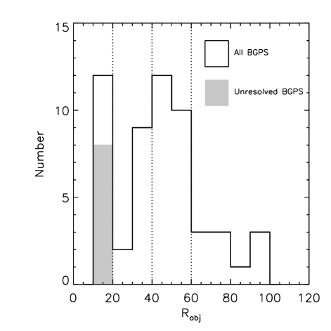
Figure 6.— The distribution of extracted source radii for all 55 BGPS sources. The white histogram marks all 55 sources while the gray histogram marks the unresolved sources for which we have set the radius to an upper-limit of the beam size. The dotted lines mark the radii of the aperture sizes used in the BGPS catalog, $R_{ap}=$ 20″, 40″, and 60″.

Figure 7.— The distribution of distances between the 55 BGPS sources out to 500″. The dotted lines mark the diameters of the apertures used in the BGPS catalog, $\theta_{ap}=$ 40″, 80″, and 120″. Only approximately 5 sources will suffer from contamination with the 120″ aperture.

Table 3Millimeter Sources

ID		BGPS ID	Group
Number	Source	Number	Number	Comments
01……..	G189.646+00.131	7469	2
02……..	G189.659+00.185	7470	2
03……..	G189.682+00.185	7471	2	IRAS 06047+2040
04……..	G189.782+00.265	7475	2	IRAS 06053+2036
05……..	G189.116+00.643	7467	1	IRAS 06052+2122
06……..	G189.788+00.281	7479	2
07……..	G189.713+00.335	7472	2
08……..	G189.789+00.291	7480	2
09……..	G189.744+00.335	7473	2
10……..	G189.782+00.323	7476	2
11……..	G189.836+00.303	7485	2	IRAS 06055+2034
12……..	G189.950+00.231	7491	2
13……..	G189.776+00.343	7474	2	S252A, IRAS 06055+2039
14……..	G189.834+00.317	7484	2
15……..	G189.888+00.303	7489	2	IRAS 06056+2032
16……..	G189.804+00.355	7481	2
17……..	G189.030+00.781	7465	1	IRAS 06056+2131
18……..	G189.831+00.343	7843	2	J06084309+2036182
19……..	G189.879+00.319	7487	2
20……..	G189.885+00.319	7488	2
21……..	G189.810+00.369	7482	2
22……..	G189.032+00.793	7466	1	IRAS 06056+2131
23……..	G189.921+00.331	7490	2
24……..	G189.015+00.823	7464	1
25……..	G188.991+00.859	7463	1
26……..	G188.948+00.883	7461	1	S252
27……..	G189.951+00.331	7492	2
28……..	G189.783+00.433	7477	2	IRAS 06059+2042
29……..	G188.975+00.911	7462	1
30……..	G189.990+00.353	7493	2
31……..	G189.783+00.465	7478	2
32……..	G188.792+01.027	7460	1	IRAS 06061+2151
33……..	G190.006+00.361	7494	2	IRAS 06061+2028
34……..	G189.864+00.499	7486	2	IRAS 06063+2040
35……..	G189.231+00.893	7468	1	IRAS 06065+2124
36……..	G190.054+00.533	7496	2	IRAS 06068+2030
37……..	G190.044+00.543	7495	2
38……..	G190.063+00.679	7497	2
39……..	G190.192+00.719	7499	2
40……..	G190.171+00.733	7498	2	IRAS 06078+2030
41……..	G190.240+00.911	7500	2	IRAS 06087+2031
42……..	G192.629-00.157	7505	3
43……..	G192.602-00.143	7503	3	S256, IRAS 06096+1757
44……..	G192.629-00.123	7504	3
45……..	G192.581-00.043	7501	3	S255N
46……..	G192.662-00.083	7507	3
47……..	G192.596-00.051	7502	3	S255IR, J06125330+1759215
48……..	G192.644+00.003	7506	3	S258
49……..	G192.719+00.043	7508	3	IRAS 06105+1756
50……..	G192.764+00.101	7509	3
51……..	G192.816+00.127	7510	3
52……..	G192.968+00.093	7511	3
53……..	G193.006+00.115	7514	3
54……..	G192.981+00.149	7512	3	J06142359+1744469
55……..	G192.985+00.177	7513	3

The spectral model has two significant differences from that of the R08 study. In particular, the inclusion of NH₃(3,3) lines in the analysis necessitates treating the ortho- and para-NH₃ states in more detail. Rather than simply adopting a full thermal equilibrium as done by R08, we treat the two sets of states as different species with an ortho-to-para ratio of 1:1, which is the high temperature limit ($T_{K}>40$ K; Takano et al. 2002). Given that the kinetic temperature derived from only the (1,1) and (2,2) lines provides a good estimate of the (3,3) line in most cases, this assumption is adequate. As such, partition functions for the two species are decoupled and contain only the ortho- and the para- states:

$$Z_{O}=$$

$$1+ \sum_{J}2(2J+1)\exp\left\{\frac{-h[BJ(J+1)+(C-B)J^{2}]}{kT_{k}}\right\}$$

$$\qquad\mbox{for }J=3,6,9,\dots$$ (2)

$$Z_{P}=$$

$$\sum_{J} (2J+1)\exp\left\{\frac{-h[BJ(J+1)+(C-B)J^{2}]}{kT_{k}}\right\}$$

$$\qquad\mbox{for }J=1,2,4,5,\dots,$$ (3)

where we have only included the metastable states given by $J=K$. The lifetimes of the non-metastable states are relatively short and the levels are not well populated. The partition functions are subject to the constraint that $Z_{O}=Z_{P}$, representing our assumption of the 1:1 ortho-to-para ratios. In addition to a different partition function, we also model the effects of the frequency switching explicitly in the model spectrum since the frequency switch is smaller than in the R08 study. We build a frequency switched version of the spectrum by shifting it $\pm 5$ MHz in frequency and subtracting half of the amplitude in the model. Thus, we fit both the peaks and the negative features in the observed spectra, resulting in a fit which is more sensitive to the low-intensity emission.

Emission from the H₂O and C₂S lines is not treated in detail by the model but rather by simply calculating its velocity-integrated intensity. Since the model is necessarily simple, complicated sources will be represented by average properties. However, the model produces good fits for the wide variety of sources found in the observations.

5. Results

Table 4Observed 1.1 mm Properties

ID		RA	Dec	peak RA	peak Dec	Rmajor	Rminor	PA	Robj	Sν(120″)	Sν(int)
number	Source	(J2000)	(J2000)	(J2000)	(J2000)	(″)	(″)	(∘)	(pc)	(mJy)	(mJy)
01……..	G189.646+00.131	06 07 30.6	20 40 00.6	06 07 30.9	20 39 46.1	33.0	19.9	74	0.50	936 (250)	988 (120)
02……..	G189.659+00.185	06 07 44.4	20 40 49.6	06 07 44.7	20 40 36.6	20.5	14.1	139	$<0.17$	1010 (270)	370 (91)
03……..	G189.682+00.185	06 07 46.9	20 39 39.6	06 07 47.5	20 39 27.4	33.5	19.2	138	0.49	1509 (300)	1700 (150)
04……..	G189.782+00.265	06 08 17.3	20 36 37.9	06 08 17.9	20 36 32.6	28.2	18.0	145	0.40	1380 (300)	1190 (140)
05……..	G189.116+00.643	06 08 19.9	21 22 26.3	06 08 19.8	21 22 29.2	31.2	19.9	4	0.49	1190 (320)	1090 (130)
06……..	G189.788+00.281	06 08 22.8	20 36 38.0	06 08 22.2	20 36 41.7	21.7	17.6	43	0.32	1630 (330)	1019 (140)
07……..	G189.713+00.335	06 08 25.4	20 42 04.8	06 08 25.1	20 42 08.9	26.3	20.6	158	0.45	1360 (300)	1160 (140)
08……..	G189.789+00.291	06 08 25.8	20 37 04.9	06 08 24.7	20 36 52.8	16.5	9.1	13	$<0.17$	1430 (330)	347 (94)
09……..	G189.744+00.335	06 08 29.0	20 41 04.7	06 08 28.8	20 40 34.5	28.6	20.9	72	0.48	2960 (420)	1960 (210)
10……..	G189.782+00.323	06 08 29.3	20 38 13.1	06 08 30.9	20 38 13.9	28.5	22.7	38	0.51	3190 (450)	2240 (220)
11……..	G189.836+00.303	06 08 30.5	20 34 33.3	06 08 33.1	20 34 49.0	34.2	23.4	142	0.59	2480 (380)	1780 (210)
12……..	G189.950+00.231	06 08 31.0	20 26 49.9	06 08 31.1	20 26 44.4	34.4	22.6	17	0.58	1670 (310)	1910 (160)
13……..	G189.776+00.343	06 08 34.4	20 39 18.2	06 08 34.6	20 39 07.7	38.5	26.8	151	0.70	8930 (850)	11100 (410)
14……..	G189.834+00.317	06 08 35.0	20 35 10.5	06 08 36.0	20 35 19.7	23.4	17.1	32	0.33	2730 (400)	1530 (170)
15……..	G189.888+00.303	06 08 38.9	20 32 06.5	06 08 39.6	20 32 05.3	20.6	13.5	165	$<0.17$	1370 (290)	537 (110)
16……..	G189.804+00.355	06 08 39.7	20 38 02.0	06 08 40.8	20 38 00.5	23.4	22.2	40	0.44	8060 (790)	4700 (320)
17……..	G189.030+00.781	06 08 40.2	21 31 00.0	06 08 40.1	21 31 00.8	26.9	22.8	85	0.50	11100 (990)	11200 (410)
18……..	G189.831+00.343	06 08 41.3	20 36 04.8	06 08 41.6	20 36 11.4	36.2	28.9	73	0.71	5780 (610)	6420 (350)
19……..	G189.879+00.319	06 08 43.2	20 33 49.9	06 08 42.2	20 32 58.4	39.2	21.9	58	0.61	2390 (350)	2400 (210)
20……..	G189.885+00.319	06 08 44.5	20 32 12.0	06 08 42.9	20 32 39.5	32.5	22.7	1	0.56	2450 (360)	2080 (200)
21……..	G189.810+00.369	06 08 44.6	20 38 18.5	06 08 44.7	20 38 06.1	54.4	31.8	66	0.95	8090 (780)	11300 (480)
22……..	G189.032+00.793	06 08 45.7	21 31 51.7	06 08 43.1	21 31 15.4	30.9	23.7	39	0.56	11100 (1000)	6690 (430)
23……..	G189.921+00.331	06 08 49.2	20 31 46.8	06 08 50.1	20 31 07.1	25.0	14.9	21	0.25	2500 (380)	697 (160)
24……..	G189.015+00.823	06 08 49.7	21 33 49.2	06 08 47.9	21 32 58.1	34.9	16.2	67	0.39	2690 (390)	1660 (190)
25……..	G188.991+00.859	06 08 53.1	21 35 32.0	06 08 53.0	21 35 16.5	30.2	12.6	51	$<0.17$	977 (270)	707 (110)
26……..	G188.948+00.883	06 08 53.4	21 38 23.8	06 08 52.9	21 38 16.9	29.0	24.4	89	0.55	12899 (1200)	14599 (450)
27……..	G189.951+00.331	06 08 53.6	20 29 37.3	06 08 53.8	20 29 32.6	53.5	34.9	157	0.99	5980 (620)	10800 (390)
28……..	G189.783+00.433	06 08 55.5	20 41 16.0	06 08 55.8	20 41 19.6	43.6	22.4	44	0.66	1439 (300)	1840 (160)
29……..	G188.975+00.911	06 09 03.6	21 38 03.8	06 09 02.7	21 37 37.5	26.6	16.2	56	0.33	718 (260)	703 (95)
30……..	G189.990+00.353	06 09 03.7	20 28 18.0	06 09 03.4	20 28 11.3	22.3	14.0	3	$<0.17$	886 (280)	499 (91)
31……..	G189.783+00.465	06 09 04.4	20 42 12.6	06 09 03.0	20 42 15.4	30.0	19.8	124	0.47	917 (270)	949 (120)
32……..	G188.792+01.027	06 09 06.7	21 50 48.5	06 09 06.0	21 50 39.1	27.2	22.2	83	0.49	4240 (570)	4650 (250)
33……..	G190.006+00.361	06 09 08.4	20 27 33.7	06 09 07.2	20 27 34.9	30.5	20.1	110	0.48	887 (260)	760 (110)
34……..	G189.864+00.499	06 09 20.7	20 39 30.8	06 09 20.6	20 39 02.7	50.2	36.5	27	0.99	3850 (450)	6969 (300)
35……..	G189.231+00.893	06 09 30.4	21 23 44.7	06 09 30.6	21 23 39.8	17.4	15.4	100	0.20	464 (260)	427 (79)
36……..	G190.054+00.533	06 09 51.1	20 30 14.5	06 09 51.7	20 30 03.2	52.7	23.4	21	0.75	2220 (340)	2930 (220)
37……..	G190.044+00.543	06 09 54.6	20 30 56.2	06 09 52.7	20 30 52.2	25.1	17.7	22	0.37	2420 (360)	1019 (170)
38……..	G190.063+00.679	06 10 27.0	20 33 48.5	06 10 25.7	20 33 45.6	20.3	12.9	149	$<0.17$	418 (230)	229 (64)
39……..	G190.192+00.719	06 10 50.3	20 27 51.6	06 10 50.5	20 28 11.4	16.4	12.1	29	$<0.17$	685 (260)	316 (74)
40……..	G190.171+00.733	06 10 51.3	20 29 57.7	06 10 51.2	20 29 38.8	45.1	16.9	32	0.49	1540 (300)	2090 (160)
41……..	G190.240+00.911	06 11 40.4	20 31 26.7	06 11 39.6	20 31 12.8	28.0	17.2	73	0.38	726 (260)	626 (98)
42……..	G192.629-00.157	06 12 33.6	17 54 48.7	06 12 33.5	17 54 40.4	21.9	16.7	57	0.30	796 (290)	558 (96)
43……..	G192.602-00.143	06 12 33.6	17 56 19.8	06 12 33.2	17 56 33.1	25.9	16.8	11	0.35	894 (300)	868 (110)
44……..	G192.629-00.123	06 12 39.8	17 55 28.8	06 12 41.0	17 55 39.2	35.6	21.3	16	0.56	709 (290)	740 (110)
45……..	G192.581-00.043	06 12 52.8	18 00 32.6	06 12 52.9	18 00 29.0	25.2	21.9	174	0.46	14600 (1300)	11400 (450)
46……..	G192.662-00.083	06 12 53.1	17 55 21.0	06 12 53.7	17 55 07.3	33.5	11.7	43	$<0.17$	565 (310)	463 (85)
47……..	G192.596-00.051	06 12 54.1	17 58 54.1	06 12 52.8	17 59 31.0	46.5	29.5	22	0.83	15400 (1400)	17300 (590)
48……..	G192.644+00.003	06 13 09.8	17 58 40.3	06 13 10.6	17 58 32.6	28.1	22.8	45	0.51	1330 (320)	1380 (140)
49……..	G192.719+00.043	06 13 28.0	17 56 02.1	06 13 28.6	17 55 41.6	43.2	27.3	120	0.76	2320 (390)	3580 (220)
50……..	G192.764+00.101	06 13 46.7	17 55 00.4	06 13 46.8	17 55 02.5	39.6	21.0	146	0.59	2020 (370)	2480 (180)
51……..	G192.816+00.127	06 13 58.8	17 52 51.2	06 13 58.8	17 53 03.0	20.1	13.2	39	$<0.17$	615 (320)	505 (84)
52……..	G192.968+00.093	06 14 08.3	17 44 04.6	06 14 09.6	17 44 03.9	25.4	16.2	166	0.32	682 (310)	620 (93)
53……..	G193.006+00.115	06 14 18.8	17 42 36.9	06 14 19.1	17 42 41.7	19.4	14.8	162	0.19	1310 (350)	661 (110)
54……..	G192.981+00.149	06 14 23.4	17 44 28.4	06 14 23.7	17 44 56.1	49.6	25.5	43	0.78	4290 (520)	6480 (290)
55……..	G192.985+00.177	06 14 30.2	17 45 34.0	06 14 30.4	17 45 31.6	18.4	14.3	85	$<0.17$	844 (320)	516 (90)

Note. — Errors are given in parentheses.

5.1. 1.1 mm Results

We have extracted 55 millimeter continuum sources from the BGPS maps. The 1.1 mm sources are listed in Table 3, along with their ID number in the complete BGPS source catalog, their corresponding group number (see §3.1.3), and any coincident IRAS sources, 2MASS sources and well known millimeter sources. Table 4 lists extracted 1.1 mm source properties including a running source ID number (column 1), the source name (based on the Galactic coordinates of the peak emission; Column 2), centroid RA and DEC (columns 3 and 4), RA and DEC of the peak emission (columns 5 and 6), size of semi-major and semi-minor axes in arcseconds (columns 7 and 8), position angle of best-fit ellipse measured counter-clockwise from the $x$-axis ($\ell=0^{\circ}$) in Galactic coordinates (column 9), the deconvolved source radius $R_{obj}$ (column 10), and $S_{\nu}$(120″) and $S_{\nu}$(int) (columns 11 and 12). Some sources are sufficiently small that a deconvolved radius cannot be determined, and we assume a source diameter equal to the beam FWHM as an upper limit on the radius for these objects.

$S_{\nu}$(int) and $R_{obj}$ adequately characterize the sources but these two quantities are highly dependent upon the source extraction algorithm and are not easily compared with other observations. In order to support comparison of our results with other studies, we will also present a flux within a well-characterized and commonly used aperture.

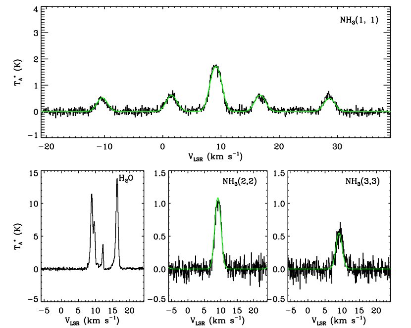
Figure 9.— H₂O,NH₃(1,1), (2,2), and (3,3) spectra for G189.776+0.343 (ID #13). Top panel: Black is observed NH₃(1,1) spectrum and green is the model fit. From left to right, the bottom panels show H₂O, NH₃(2,2) and NH₃(3,3) spectra. Figures 8b-at are available in the online version of the Journal.

To evaluate which aperture most closely represents the true mm flux, we consider the derived object radii as well as the distance between all BGPS sources. Figure 6 shows the distribution of derived source radii for the 55 BGPS sources (white histogram) and the unresolved sources where we have assigned the beam size as an upper-limit for the source radius (gray histogram). The dotted lines mark the radii of the apertures in which we present photometry in the BGPS catalog. There is a large spread in the object radii, with the largest being almost 100″. Figure 7 shows the distribution of angular separation between the emission maxima of all 55 BGPS sources out to 500″. The dotted lines mark the diameters of our chosen apertures.

To characterize the mm flux well, we should choose an aperture size greater than the largest source radius yet small enough to reduce the number of sources which will include flux from their neighbors. If we choose an aperture much larger than the source and no other mm sources fall within that aperture, then the flux will still be representative of the total mm flux since the background averages to zero. The distribution of source sizes supports the use of the 120″ aperture, which is only smaller than 10 of the 55 BGPS sources. Figure 7 shows that for the 120″ aperture, only approximately 5 source fluxes will be contaminated by emission from nearby sources.

We have chosen to present the $S_{\nu}$(120″) fluxes as well-characterized fluxes for comparison with other studies. We present masses calculated from both $S_{\nu}$(120″) and $S_{\nu}$(int). However, when calculating physical properties which are highly dependent upon size, such as the volume and surface densities, we will present $S_{\nu}$(int) and use the derived source radius as the physical size.

Figure 10.— The white histogram denotes the distance between each of the 46 cross-matched NH₃ pointings and the peak of the associated BGPS source. The striped histogram marks the distance between the peak in 1.1 mm emission and the nearest NH₃ pointing for the 34 BGPS sources in the full sample. The NH₃ pointings were chosen by eye from preliminary BGPS images, which can account for the offsets larger than the beam size in the striped histogram. The large distances in the white histogram result from multiple NH₃ pointings per BGPS source, with typical spacings between pointings on order of the GBT beam size (31″) or larger.

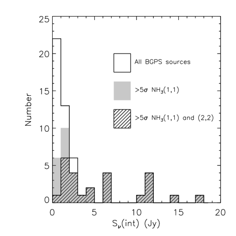
Figure 11.— Distribution of $S_{\nu}$(120″) (left) and integrated flux densities, $S_{\nu}$(int) (right). The white histograms include all extracted 1mm sources, the gray histograms represent the full sample (all sources with a $>5\sigma$ detection in NH₃(1,1)), and the striped histograms represent subset 1 (all sources with a $>5\sigma$ detection in NH₃(1,1) and (2,2)).

5.2. NH₃ Results

Example spectra of the NH₃(1,1), (2,2), (3,3) and H₂O lines are shown in Figure 9 for the source G189.776+00.343 (ID #13). Spectra for all NH₃ pointings are shown in Figures 8b$-$at in the online materials. NH₃(4,4) and C₂S were not observed for many sources and are not shown here. We detected a $>5\sigma$ NH₃(1,1) line in 95% (53 of 56) of all NH₃ pointings, and 60% (33) of the pointings had at least a 5$\sigma$ detection in both the (1,1) and (2,2) lines, where a $5\sigma$ detection means the integrated intensity is greater than 5 times the measured error in the integrated intensity for each source.

5.3. Combined 1.1 mm and NH₃ Results

Each NH₃ pointing was assigned to a single distinct BGPS source. Of the 55 BPGS sources, 37 have ammonia observations along a line of sight that intersects the source. Three BGPS sources have an ammonia pointing associated with the source that lacks any discernible NH₃(1,1) emission. In the remaining 34 BGPS sources, there may be multiple NH₃ pointings within the contours of the BGPS source, and the NH₃ pointings do not necessarily correspond to either the centroid or peak coordinates of each BGPS source because they were chosen by eye prior to completion of the final BGPS maps. We exclude the seven NH₃ pointings that do not fall within the contours of an extracted BGPS source from the analysis. These pointings correspond to low significance BGPS sources. The seven pointings all have significant NH₃(1,1) emission, indicating that many marginal detections in the BGPS not included in the catalog are likely real.

In this analysis we will consider only the NH₃ pointing which is located closest to the peak of the millimeter emission. The angular separation between the closest NH₃ pointing and the peak of the millimeter emission is shown in Figure 10. The white histogram includes all NH₃ pointings while the striped histogram includes only the NH₃ pointings closest to the millimeter peak. Most of the NH₃ pointings assigned to a BGPS source are located less than a FWHM beam away from the millimeter peak.

We define a “full sample” which consists of 34 BGPS sources that have at least a 5$\sigma$ detection in the NH₃(1,1) transition. Sources without a 5$\sigma$ detection in the NH₃(2,2) transition can only provide an upper-limit to the derived gas properties such as $T_{K}$. Consequently, the full sample can only characterize upper-limits for these properties. We also define “subset 1” which is comprised of 25 BGPS sources with a $>5\sigma$ detection in both the NH₃(1,1) and (2,2) transitions. However, subset 1 may not be characteristic of the faint end of the full sample. Due to the complementary properties of each sample, we will present the characteristics of both. For clarity, we point out that subset 1 is entirely contained in the full sample.

Observed properties of NH₃ pointings in the full sample are given in Table 5, including the source ID (column 1), specific coordinates of the NH₃ pointing which do not necessarily correspond to the peak of the millimeter emission (Columns 2 and 3), radial velocity and Gaussian $1/e$ line width (columns 4 and 5), and main beam temperature and integrated intensities for the NH₃(1,1), (2,2), (3,3) and (4,4) transitions (columns 6-13). For undetected lines, we present upper-limits for the main beam temperature and integrated intensities given as $T_{\rm mb}$$<5$ RMS and $W<5$ RMS $\Delta v/\sqrt{(}N)$, where RMS is the noise per channel of each spectrum, $\Delta v$ is the channel width in velocity, and $N$ is the number of channels used to calculate the RMS.

Table 6 lists derived gas properties including the measured optical depth of the (1,1) transition (column 2), kinetic gas temperature (column 3; see §6.2), excitation temperature of the NH₃(1,1) transition (column 4), derived sound speed and non-thermal velocity dispersion ($a$ and $\sigma_{NT}$; columns 5 and 6; see §6.3), and flags for detection or non-detection of the H₂O and CCS lines (columns 7 and 8). The additional 12 NH₃ pointings are included in Tables 5 and 6, but are not included in the general analysis. Numbers given in parentheses are errors in the same units as each column.

The distributions of the flux densities, $S_{\nu}$(120″) and $S_{\nu}$(int), are shown in Figure 11. The white histogram includes all 55 BGPS sources extracted from the millimeter maps. The gray histogram includes all BGPS sources included in the full sample ($>5\sigma$ detection in NH₃(1,1)), while the striped histogram denotes subset 1 ($>5\sigma$ detection in NH₃(1,1) and (2,2)). The faintest sources are excluded from subset 1, as expected.

Figure 12 plots the peak $T_{\rm mb}$ of the (2,2) transition versus the peak $T_{\rm mb}$ of the (1,1) transition. Pointings with $<5\sigma$ detection in the (2,2) transition are shown as upper limits. The fainter lines in (1,1) are typically the pointings with a weak or non-detection of (2,2). The weaker BGPS sources typically have weaker NH₃(1,1) detections and only upper-limits for the NH₃(2,2) line.

Figure 12.— Peak main beam temperature of the NH₃(1,1) line versus the (2,2) line. Sources in subset 1 are marked by solid circles. Sources excluded from subset 1 give only upper limits for the (2,2) transition and are marked by arrows.

Figure 13.— Left: Velocity with respect to the LSR versus Galactic Longitude. Groups 2 and 3 span the same velocity range, while Group 1 is found at lower velocities. Right: Distribution of velocity dispersions. The white histogram marks the full sample and the dashed histogram marks subset 1. The dashed line marks the spectral resolution of the NH₃ spectra, 0.08 km s^-1.

5.4. Maser Activity

We also obtained observations of the 22 GHz water maser in conjunction with our GBT NH₃ observations. Eight of the 34 BGPS sources presented here have water maser emission (see columns 7 and 8 of Table 6). Of these, only Sources #16 and #24 have not been reported previously as maser sources. The remaining 6 BGPS sources with maser activity were previously known to exhibit water as well as some SiO or methanol maser activity in a $1^{\prime}$ region around the observed GBT position based on a SIMBAD search. The fraction, $8/34=0.2$, can be regarded as a lower limit as two sources, #13 and #47, show maser emission along one line of sight but not another line of sight through the same core. Since the GBT ammonia spectroscopy was not complete mapping, some sources may have maser emission elsewhere in the object. However, the masing lines of sight are those nearest the peaks of the BGPS emission, so the lower limit is likely representative of the true fraction. For comparison, Szymczak et al. (2005) find a detection fraction of water masers of 0.52 using 6.7 Ghz methanol masers, associated with massive young stellar objects, as a prior. Similarly, Chambers et al. (2009) find detection rates of 0.16, 0.54 and 0.59 for water masers in their IRDC cores classified with Spitzer data as “quiescent,” “red” and “active” respectively. The BGPS-selected water maser detection fraction is most similar to the detection fraction in “quiescent” IRDCs determined by Chambers et al. (2009). We see no evidence for maser activity in the NH₃(3,3) transition. All (3,3) spectra are consistent with the temperatures and line widths determined in conjunction with the (1,1) and (2,2) states. We defer further discussion of the water maser detection fraction to a later paper (M. K. Dunham et al., in prep).

6. Analysis

6.1. Radial Velocities and Distances

We adopt the VLBI parallax distance to S252 of $2.10\pm 0.026$ kpc (Reid et al. 2009) for the entire sample of BGPS sources. The radial velocities observed in the NH₃ spectra are listed in Table 5 (column 4), and are shown in Figure 13. Filled circles mark sources in Subset 1, while the crosses mark sources without a 5$\sigma$ detection in the NH₃(2,2) line. The sources excluded from Subset 1 are spread evenly in velocity space, as expected since the weaker BGPS sources should not be preferentially located at any given radial velocity. Toward the Galactic anti-center (as well as all Cardinal points: $l=0^{\circ},90^{\circ},180^{\circ},$ and $270^{\circ}$), radial velocities expected from purely circular rotation are 0 km s^-1, rendering kinematic distances unsound. A non-zero radial velocity along these lines of sight is most likely due to the peculiar motions of individual gas clouds rather than galactic rotation.

From Figure 13, it is apparent that groups 2 and 3 span the same velocity range (5 to 10 km s^-1) while group 1 is found at slightly lower radial velocities ($-$1 to 4 km s^-1). Although there is no evidence in our data that these groups are related, surveys of lower density tracers (such as CO and ¹³CO) toward S247 and S252 (groups 1 and 2) show evidence of interaction between the two HII regions. Kömpe et al. (1989) mapped the S247/252 complex in ¹³CO ($J=1-0$) transition with a beam-sampled map at 4′ resolution and found a bridge connecting the two clouds. Specifically, the bulk of the material towards S247 is found between velocities of $-$1 km s^-1 and 5 km s^-1 with a tail extending to velocities of up to 10 km s^-1, which overlaps the S252 region in velocity space (see Figure 7 in Kömpe et al. 1989). Carpenter et al. (1995a) mapped a larger region including the S247 and S252 complexes in ¹³CO($J=1-0$) and found three distinct filaments. Two filaments with radial velocities of $\sim$2 km s^-1 wrap around S247, while the third filament, at a radial velocity of $\sim$10 km s^-1, extends to the S252 region. It is clear that the S247 and S252 regions (groups 1 and 2) are interacting, justifying our application of the VLBI parallax distance to our entire sample regardless of the difference in radial velocities between the groups of sources.

Not all sources will be at precisely the parallax distance; however, we account for variation in the distances by including a larger error than the parallax distance error. Since it is clear that groups 1 and 2 are part of filaments wrapping around and interacting between S247 and S252, we will consider the size of the HII regions when determining the spread in distance. S247 has a diameter of 9′ and S252 has a diameter of 40′ (Sharpless 1959). If the cloud between Groups 1 and 2 is assumed to be spherically symmetric, its angular size on the sky can provide an estimate of the distance along the line of sight. Since it is apparent that groups 1 and 2 are interacting, we will consider a sphere of approximately 100′ in diameter that encompasses both groups 1 and 2 and the associated HII regions, and corresponds to a distance uncertainty of 0.061 kpc. We will assume the spread in distance is approximately equal to the 100′ diameter, and will assign that to the distance error to account for the case where the parallax source is found at the extreme edge of the region and note that this is likely a minimum estimate of the error.

6.2. Kinetic Temperature

The kinetic temperatures derived from the NH₃ observations are given in column 3 of Table 6. The uncertainties in individual determinations of $T_{K}$ are small, with $\mbox{$\langle\sigma_{\mbox{$T_{K}$}}/\mbox{$T_{K}$}\rangle$}=0.04$. In this and subsequent analyses, the uncertainties quoted are the standard deviation about the mean of the sample, rather than the uncertainty in the mean. For sources without a 5$\sigma$ detection in NH₃(2,2) the derived kinetic temperature is an upper-limit, and thus the mean kinetic temperature for the full sample is only an upper-limit. The distribution for the full sample is characterized by $\langle$$T_{K}$$\rangle<19.4\pm 4.9$ K, while the distribution for Subset 1 is characterized by $\langle$$T_{K}$$\rangle=20.6\pm 5.1$ K. The mean limit on kinetic temperature for the sources without a 5$\sigma$ NH₃(2,2) detection is $\langle$$T_{K}$$\rangle<16.1\pm 2.3$ K. As some property distributions may be non-Gaussian, the uncertainty should be regarded primarily as an indicator of the scatter in the sample. The dispersion about the mean kinetic temperature for the full sample is thus six times larger (0.24) than the fractional uncertainties in individual temperatures, so the differences among sources are real.

Zinchenko et al. (1997) mapped 17 molecular clouds associated with FIR sources in NH₃(1,1) and (2,2) and found that $T_{K}$ increases toward the peak of the NH₃ emission. Additionally, Friesen et al. (2009) have shown that NH₃ emission closely follows mm continuum emission. Since our NH₃ pointings are located near the peak of the mm emission, which corresponds to the NH₃ peak as well, the mean $T_{K}$ is likely smaller than the peak $T_{K}$ we report.

6.3. Velocity Dispersion and Non-Thermal Pressures

The line-width provides a measure of the one-dimensional velocity dispersion within each source. Rosolowsky et al. (2008) found velocity dispersions ranging from 0.07 to 0.7 km s^-1 for the NH₃(1,1) and (2,2) lines of low-mass star-forming cores in the Perseus molecular cloud, and they suggest that there is evidence of multiple velocity components in all sources with $\sigma_{v}>$ 0.2 km s^-1. The velocity dispersions are listed in column 5 of Table 5 and the distribution of our sample is shown in Figure 13. In contrast to the low-mass sources in Perseus, our distribution has a tail extending up to a high velocity dispersion $\sigma_{v}\approx$ 1.3 km s^-1.

The observed velocity dispersion is a combination of the thermal and non-thermal motions of the gas. In order to calculate the non-thermal contribution, $\sigma_{NT}$, we simply remove the thermal contribution:

$$\sigma_{NT}=\sqrt{\sigma_{v}^{2}-\frac{k\mbox{$T_{K}$}}{17m_{H}}},$$ (4)

where $(k\mbox{$T_{K}$}/17m_{H})^{1/2}$ is the thermal broadening due to NH₃ and $17m_{H}$ is the mass of a single ammonia molecule. The non-thermal velocity dispersion ranges from 0.37 km s^-1 to 1.3 km s^-1 with a mean of $0.72\pm 0.25$ km s^-1 for subset 1. We can compare $\sigma_{NT}$ to the predicted thermal sound speed of the gas given by $a=(k\mbox{$T_{K}$}/\mu m_{H})^{1/2}$, where $\mu=2.37$. The thermal sound speed for subset 1 ranges from 0.22 km s^-1 to 0.34 km s^-1 with a mean of 0.27$\pm$0.03 km s^-1. The mean Mach number is then 2.8. Both $a$ and $\sigma_{NT}$ are listed in Table 6 (columns 5 and 6). The corresponding ratio of $\sigma_{NT}$ to $a$ ranges from 1.5 to 4.2 with a mean of 2.7$\pm$0.8. The non-thermal velocity dispersion is shown in Figure 14 versus $T_{K}$. The solid line plots the thermal sound speed, $a$, as a function of $T_{K}$. In all sources, the non-thermal velocity dispersion is much larger than the thermal velocity dispersion and the discrepancy increases with $T_{K}$.

There is no apparent correlation between $\sigma_{NT}$ and source size or mass. However, there is a correlation between the position of a source within its group and $\sigma_{NT}$. Figure 15 displays the position of each source in Galactic coordinates and the symbol size denotes the magnitude of $\sigma_{NT}$. For Group 2, the highest values of $\sigma_{NT}$ are found at the center of the cluster. A similar statement could be made for Group 3, but there it is difficult to definitively say, due to the smaller number of sources.

Figure 14.— The non-thermal velocity dispersion, $\sigma_{NT}$, versus derived kinetic temperature. Arrows indicate upper limits for the kinetic temperatures. Solid line denotes the thermal sound speed given by $a=\sqrt{kT/\mu m_{H}}$.

6.4. Virial and Isothermal Masses

Combining heterodyne and dust continuum observations provides estimates of both virial mass and total gas and dust mass. Total gas and dust mass (also called the isothermal mass, $M_{iso}$, due to the simplifying assumption that the dust can be characterized by a single temperature) is given by

$$M_{iso} =\frac{S_{\nu}D^{2}}{\kappa_{\nu}B_{\nu}(T_{d})}$$

$$=13.1\ \mbox{M${}_{\odot}$}\ \left(\frac{S_{\nu}}{1\ Jy}\right) \left(\frac{D}{1\ kpc}\right)^{2}\left(\frac{e^{13.0\ K/T_{d}}-1}{e^{13.0\ K/20.0\ K}-1}\right),$$ (5)

where $S_{\nu}$ is flux density, $D$ is the distance, $\kappa_{\nu}$ is the dust opacity per gram of gas and dust, and $B_{\nu}$ is the Planck function evaluated at a dust temperature, $T_{d}$. We logarithmically interpolate the Ossenkopf & Henning dust opacities (1994, Table 1, column 5, commonly referred to as OH5 dust) to the effective central frequency of the Bolocam bandpass convolved with a 20 K blackbody modified by an opacity varying with frequency as $\kappa_{\nu}\propto\nu^{1.8}$ (271.1 GHz; Aguirre et al. 2010) and obtain $\kappa_{\nu}=0.0114$ cm² g^-1.

We assume the gas and dust are collisionally coupled, make the simplifying assumption that $T_{d}=\mbox{$T_{K}$}$ and use $T_{K}$ derived from the NH₃ observations. Evans, Blair, & Beckwith (1977) observed the S255 molecular cloud in ¹²CO, ¹³CO, H₂CO, and 2.2 $\mu$m emission. They studied the gas and dust energetics and concluded that the primary energy flow is through infrared dust emission and that an embedded source and the exciting stars of the many nearby HII regions are the likely heat sources for the cloud. Dust typically controls the energetics in the dense interior of the star-forming regions where the density is high enough to shield the gas from the ultraviolet radiation in the interstellar radiation field (ISRF) and also to transfer energy from the dust to the gas via collisions (Goldreich & Kwan 1974, Evans et al. 2001). Towards the outer edges of the clump the density is much lower, and the gas is no longer collisionally coupled to the dust. The gas is also now subject to the ultraviolet portion of the ISRF, allowing the gas kinetic temperature to rise above the dust temperature (see Figure 9 in Mueller et al. 2002). The BGPS observations probe all of these regions, and detailed models will be needed to include temperature gradients. For now, we rely on previous modeling (e.g., Mueller et al. 2002, Shirley et al. 2002) to support the assumption that $T_{d}=\mbox{$T_{K}$}$ on average.

Figure 15.— Galactic longitude versus Galactic latitude for the full sample. Symbol size denotes the magnitude of the non-thermal velocity dispersion, $\sigma_{NT}$.

As discussed in §6.2, our single measurement of $T_{K}$ likely corresponds to the maximum temperature seen within the BGPS source. Thus, using $T_{d}=\mbox{$T_{K}$}$ to describe the dust temperature for the entire source will result in a lower-limit for the isothermal mass. Zinchenko et al. (1997) find a maximum $T_{K}$ of 28 K at the peak of the NH₃ emission, and a minimum $T_{K}$ of 15 K at the edge of the NH₃ emission. This difference in temperatures corresponds to a factor of 2.3 increase in mass if the minimum temperature is assumed to be $T_{d}$. If we assume mean values from Zinchenko et al. (1997) of $T_{K}$=24 and 17.5 K, the mass would increase by a factor of 1.5 assuming the minimum temperature as $T_{d}$ rather than the maximum. If we are observing the maximum $T_{K}$ then our calculated values of $M_{iso}$ are likely to underestimate the mass by a factor of up to approximately 2.

The virial mass for a spherical, uniform density gas cloud is given by

$$M_{vir}=\frac{5\sigma_{v}^{2}R}{G},$$ (6)

where $\sigma_{v}$ is the Gaussian 1/$e$ width of the line (model fit for the velocity dispersion), $R$ is the source radius, and $G$ is the gravitational constant. We assume that the velocity dispersion measured with our single NH₃ pointing is also applicable at the edge of the 1.1 mm continuum emission, and use the single measured value in conjunction with the mm-derived object radius, $R_{obj}$, to calculate the virial mass. This assumption is supported by Friesen et al. (2009) who found that NH₃ emission closely traces 850 $\mu$m continuum emission and covers the same spatial extent as the cold dust producing the continuum emission. However, Zinchenko et al. (1997) found that the ammonia line width increased toward the peak of the NH₃ emission for about half of their sample. Thus, we are likely overestimating the virial mass by using the line width measured near the peak.

$M_{vir}$, $M_{iso}$(120″), and $M_{iso}$(int) are given in Columns $2-4$ of Table 7. For Subset 1, the isothermal masses within a 120″ aperture range from 47 M_⊙ to 610 M_⊙ with a mean of 280$\pm$180 M_⊙. Similarly, $M_{iso}$(int) ranges from 33 M_⊙ to 850 M_⊙ with a mean of 300$\pm$220 M_⊙. The virial masses range from 33 M_⊙ to 560 M_⊙  with a mean of 220$\pm$160 M_⊙. The distributions of $M_{iso}$(120″) and $M_{iso}$(int) are shown in Figure 16. The mean $M_{vir}$ to $M_{iso}$(int) ratio is 0.96$\pm$0.93 for Subset 1. The ratio of $M_{vir}$ to $M_{iso}$(int) is shown versus $M_{iso}$(int) in Figure 17. The dashed line marks the mean ratio of 1.0. The trend of decreasing $M_{vir}$/$M_{iso}$ reflects the dependence of the ratio on the inverse of the source size at a given distance. $R_{obj}$ increases with $M_{iso}$(int) which lowers $M_{vir}$/$M_{iso}$ as a function of $M_{iso}$(int).

In these calculations we have made the simplifying assumption that the density is uniform. However, if the emission is not spherical or if the density follows a power-law the virial mass will differ. A corrected virial mass is given by

$$M_{vir}=\frac{5\sigma_{v}^{2}R}{a_{1}a_{2}G},$$ (7)

$$a_{1}=\frac{1-p/3}{1-2p/5}\ \mbox{for}\ p<2.5,$$ (8)

(Bertoldi & McKee 1992) where $a_{1}$ is the correction for a power-law density distribution, $a_{2}$ is the correction for a non-spherical shape, and $p$ is the density power-law index from $n(r)=n_{f}(r/r_{f})^{-p}$ (Mueller et al. 2002). The mass ratio is then given by

$$\frac{M_{vir}}{M_{iso}}=\frac{\sigma_{v}^{2}\theta_{rad}B_{\nu}(T_{d})\kappa_{\nu}}{2GS_{\nu}Da_{1}a_{2}}\propto\frac{\kappa_{\nu}}{Da_{1}a_{2}}.$$ (9)

The mean aspect ratio of our sources is $\langle R_{maj}/R_{min}\rangle=1.5\pm 0.3$, which gives $a_{2}$ = 1.1. To estimate the effect of a power-law density distribution, we adopt the mean power-law index found by Mueller et al. (2002), $\langle p\rangle=1.8\pm 0.4$, which was derived by modeling the emission from 31 massive star-forming regions, and find $a_{1}=1.43\pm 0.34$. If the corrections for a power-law density distribution (Equation 8) and for a non-spherical shape are included, then $\langle M_{vir}/M_{iso}\rangle$ would be decreased by 36% to 0.61$\pm$0.59 for Subset 1. However, since we do not have accurate values of the power-law index for our individual sources, we will not include the correction in our calculations or subsequent discussion. Magnetic fields are also excluded from our virial mass calculation, but if magnetic fields provide additional support to the cloud, then the true mass would be larger than given by Equations 6 or 7.

The observed scatter in $M_{vir}$ to $M_{iso}$ (Figure 17) could be a result of deviations from the assumed distance of 2.10 kpc or deviations from Equation 6 due to different power-law density distributions or source ellipticities, all of which could differ from source to source and produce the observed scatter. Additional assumptions which could produce the observed scatter include the assumptions that the sources are virialized and that the velocity dispersion measured at the peak of the mm emission is also valid at $R_{obj}$. A virial parameter, $M_{vir}$/$M_{iso}$, of 1 suggests that both mass estimates are reasonable.

Figure 16.— Distributions of derived $M_{iso}$ derived from $S_{\nu}$(120″) (left) and $S_{\nu}$(int)(right). The white histogram marks the full sample and the striped histogram marks subset 1.

6.5. Volume and Surface Densities

Average particle density and average surface density can be calculated based on a mean particle weight per H nucleus ($\mu_{p}$=2.37) and a total mass within a given physical size, assuming a uniform density. We assumed a spherical volume given by $4\pi R_{obj}^{3}/3$. Mean number densities of particles and mass surface densities were calculated for each source (see Column 5 of Table 7). For Subset 1, $n_{p}$(int) ranges from $1.4\times 10^{3}$ cm^-3 to $17.0\times 10^{3}$ cm^-3 with a mean of $6.2\pm 4.4\times 10^{3}$ cm^-3, and the characteristic values for the full sample are given in Table 8.

The distribution of derived surface densities, $\Sigma$(int), ranges from 0.019 g cm^-2 to 0.13 g cm^-2 with a mean of 0.055$\pm$0.032 g cm^-2, for Subset 1. The mean surface density for the full sample is 0.048$\pm$0.030 g cm^-2  or 230$\pm$140 M_⊙ pc^-2 which is similar to the gas surface density threshold for star-formation of 200 M_⊙ pc^-2 seen in nearby, low-mass star-forming clouds (A. Heiderman et al., in prep.). This similarity supports the idea that our BGPS sources are sites of star formation, while the low volume densities imply we are detecting the less dense, larger scale portions of clumps rather than the higher density cores.

There is also evidence that a few of the BGPS clumps in this region include multiple higher density sources when observed with interferometers (see §7). Eight of the 34 BGPS cores also have water maser emission (see Table 6) which requires densities greater than $10^{10}$ cm^-3 (Strelnitskij et al. 1984; Elitzur et al. 1989), suggesting that the clumps contain much higher density substructure.

6.6. Excitation Temperature

The measured excitation temperatures are plotted against the kinetic temperatures in Figure 18. The filled circles represent Subset 1, and the corresponding distribution is characterized by $\langle$$T_{\rm ex}$(1,1)$\rangle=7.8\pm 5.6$ K. There are two sources where the best fitting model requires the limiting case $T_{\rm ex}$$=$$T_{K}$, and higher quality data would be needed to constrain $T_{\rm ex}$.

The mean difference between kinetic and excitation temperatures for Subset 1 is $\langle$$T_{K}$$-$$T_{\rm ex}$$\rangle=12.8\pm 4.5$ K. There are two possible explanations for the differences in derived temperatures. The first possibility is inherent in the way we measure the excitation temperature. As described in §4.2, in order to calculate $T_{\rm ex}$ we must assume something about the ratio of the solid angle of the source to that of the beam, which here we set to unity. A lower excitation temperature could be artificially induced by over-estimating the beam filling factor.

Another possible explanation is the density in the region. The level populations are determined by both collisional and radiative processes which depend on the local density. Pavlyuchenkov et al. (2008) study the conditions under which molecular rotational lines form using radiative transfer simulations of CO(J=2$-$1) and HCO⁺(J=1$-$0), and define a thermalization density $n_{th}$, where $T_{\rm ex}$ is within 5% of $T_{K}$. At densities greater than $n_{th}$, collisions regulate the level populations by both exciting and de-exciting molecules. A commonly used measure is the critical density, defined by $n_{crit}=A/\gamma$, where $A$ is the spontaneous emission rate and $\gamma$ is the collision rate coefficient. For low frequency transitions, such as the NH₃ inversion lines, collisions are negligible for $n<n_{crit}$, and the excitation temperature is set by the cosmic background radiation. At intermediate densities where $n_{crit}<n<n_{th}$, the excitation temperature is set by both collisions and radiation and is equal to neither the background radiation temperature nor the kinetic temperature.

Using an LVG code (Snell et al. 1984), we calculate $T_{\rm ex}$ as a function of density for a gas temperature of $T_{K}$$=20$ K, with $N(\mbox{{\rm NH}${}_{3}$})=10^{14.5}$ cm^-2, over a density range of 100$-10^{8}$ cm^-3. We assume a line width of 0.75 km s^-1 to include radiative trapping. Figure 19 plots $T_{\rm ex}$ as a function of volume density for the NH₃(1,1) transition.

From these models we find $n_{th}=210n_{crit}$ for the NH₃(1,1) transition. The large difference in $n_{crit}$ and $n_{th}$ for the NH₃ transitions is due to the low Einstein A coefficient and the importance of stimulated processes to the level populations. For comparison, Evans (1989) finds $n($$T_{\rm ex}$$=0.9$$T_{K}$$)=1.33n_{crit}$ for the CS(3-2) transition. Although this criterion is less stringent than $n_{th}$, it demonstrates the differences between the low frequency radio transitions and higher frequency submillimeter transitions. The low frequency transitions, such as the NH₃ transitions, require a density much higher than the critical density before $T_{\rm ex}$ begins to approach $T_{K}$.

Although the volume-averaged densities derived from the millimeter continuum are approximately equal to the critical densities for both the NH₃(1,1) and (2,2) transitions ($1.8\times 10^{3}\mbox{cm}^{-3}\ \mbox{and\ }2.1\times 10^{3}\ \mbox{cm}^{-3}$ respectively; Tielens 2005), the densities are not high enough for the gas to be completely thermalized, and $T_{\rm ex}$$<$$T_{K}$ as expected at densities near the critical density.

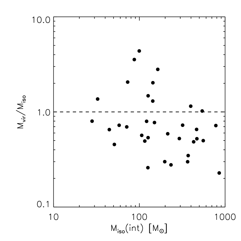
Figure 17.— Virial parameter ($M_{vir}$/$M_{iso}$) versus $M_{iso}$(int). The dashed line marks the mean virial parameter of 1.

6.7. NH₃ Excitation Density

If we assume the gas is not in LTE, we can define the excitation density, $n_{ex}$, as the density required to produce level populations described by $T_{\rm ex}$ for a given gas kinetic temperature. We calculate $n_{ex}$ from $T_{K}$, $T_{\rm ex}$, and $\tau$ via the balance of a two-level system. The excitation density is given by (Foster et al. 2009; Swift et al. 2005; Caselli et al. 2002)

$$n_{ex}=\frac{k(J(\mbox{$T_{\rm ex}$})-J(T_{cmb}))}{h\nu_{(1,1)}(1-J(\mbox{$T_{\rm ex}$})/J(\mbox{$T_{K}$}))}n_{crit}\beta,$$ (10)

where

$$J(T)=\frac{h\nu_{(1,1)}}{k(1-e^{-h\nu_{(1,1)}/kT})}.$$ (11)

$T_{cmb}=2.73$ and the escape probability is given by $\beta=(1-e^{-\tau})/\tau$, where we take $\tau=\tau_{(1,1)}\times 0.233$ which is the maximum optical depth in a single hyperfine line of the NH₃(1,1) transition.

The excitation densities are listed in Column 6 of Table 7. We cannot calculate $n_{ex}$ for the two sources where we set $T_{\rm ex}$=$T_{K}$ (see §6.6). The excitation densities for Subset 1 range from $2.1\times 10^{3}$ cm^-3 to $29.9\times 10^{3}$ cm^-3 with a mean of $9.6\pm 7.1\times 10^{3}$ cm^-3. Figure 20 shows a comparison of the NH₃ excitation density and the volume-averaged density ($n_{p}$) from the millimeter data. The solid line marks a one-to-one correlation, and is not a fit to the data. Although there is considerable spread, $n_{p}$ is in good agreement with the excitation density. The mean ratio of $n_{p}$(int) to excitation density is $1.7\pm 1.0$ with a median of $1.8$ for subset 1. The agreement between $n_{ex}$ and $n_{p}$ provide additional support that the NH₃ and continuum emission trace the same physical region.

Figure 18.— Excitation temperature of the NH₃(1,1) transition versus kinetic temperature for the full sample. The filled circles mark subset 1, and crosses mark sources with upper limits in T${}_{\mbox{kin}}$. The dashed line marks a one to one correlation but is not a fit to the data.

6.8. Column Densities

The column density per beam of NH₃ in the (1,1) state can be calculated from the observed parameters via the following equation:

$$N(1,1)=2\ \frac{8\pi\nu_{(1,1)}^{2}}{c^{2}}\frac{g_{1}}{g_{2}}\frac{1}{A_{(1,1)}}\left[1-e^{\frac{h\nu_{(1,1)}}{kT_{ex}}}\right]^{-1}\int\tau(\nu)d\nu,$$ (12)

where

$$\int\tau(\nu)d\nu= \tau(1,1)\int d\nu\ \sum_{i}s_{i}\ \exp^{-\frac{(\nu-\nu_{i}-\nu_{v_{LSR}})^{2}}{2\sigma_{i}^{2}}}$$

$$= \sqrt{2\pi}\frac{\sigma_{v}}{c}\nu_{(1.1)}\tau(1,1)$$ (13)

and $\nu_{(1,1)}$ is the central frequency of the (1,1) transition, $\tau_{(1,1)}$ is the total optical depth in the (1,1) transition, $g_{1}$ and $g_{2}$ are the statistical weights of the upper and lower levels of the (1,1) inversion transition and are equal, $A_{(1,1)}=1.68\times 10^{-7}\ \mbox{s}^{-1}$ is the Einstein A coefficient for the transition (Pickett et al. 1998), and $\sigma_{v}$ is the Gaussian $1/e$ line width. The leading factor of 2 in equation 12 assumes an equal number of NH₃ molecules in each state of the inversion transition, which is justified since the states have equal statistical weight and are separated in energy by 0.05 K. The total optical depth in the (1,1) transition is split over the 18 hyperfine components, which is expressed in the summation in Equation 13. $s_{i}$ is the weight of each hyperfine component, $\nu_{i}$ is the frequency of each hyperfine component, and $\sigma_{i}$ is the Gaussian $1/e$ width of each hyperfine component.

The total NH₃ column density, $N_{NH_{3}}$, can be calculated by scaling $N(1,1)$ by $Z/Z(J=1)$ where Z is the partition function given in Equations 2 and 3, $Z(J=1)$ is the population in only the $J=1$ level, and we truncate the summation at 50 terms. The NH₃ column densities are given in column 8 of Table 7. $N_{NH_{3}}$ ranges from $4.2\times 10^{13}$ cm^-2 to $75.8\times 10^{13}$ cm^-2 with a mean of $3.5\times 10^{14}$ cm^-2 for subset 1.

We can also calculate the column density of H₂ via the millimeter dust observations. From the gas and dust mass within a given aperture, we can calculate $N_{H_{2}}$ by

$$N_{H_{2}}=\frac{\mbox{$M_{iso}$}}{\mu_{H_{2}}m_{H}\pi R_{obj}^{2}},$$ (14)

where $\mu_{H_{2}}=2.8$. $N_{H_{2}}$ is listed in column 9 of Table 7. $N_{H_{2}}$ ranges from $4.1\times 10^{21}$ cm^-2 to $27.1\times 10^{21}$ cm^-2, with a mean of $1.2\pm 0.7\times 10^{22}$ cm^-2. Using the relationship between H₂ column density and visual extinction of Bohlin et al. (1978) assuming $R_{V}=3.1$, $N_{H_{2}}/A_{V}=9.4\times 10^{20}$ cm^-2 mag^-1, we find $A_{V}=12.4$ mag for the mean H₂ column density of our sample. However, $R_{V}=3.1$ may not be an accurate description of the dust in these dense regions. Chapman et al. (2009) find that regions with $A_{K}>1$ mag ($A_{V}>5$ mag) are described well by a $R_{V}=5.5$ extinction model (Weingartner & Draine 2001). Using this extinction model, $N_{H_{2}}/A_{V}=(2\times 1.086C_{ext})^{-1}$, where the factor of two converts $N_{H}$ to $N_{H_{2}}$ and $C_{ext}$ is the extinction cross section in the V band. Using $N_{H_{2}}/A_{V}=6.86\times 10^{20}$ cm^-2 mag^-1 we find $A_{V}=17.5$ for the mean column density of our sample.

We can obtain a measurement of the NH₃ abundance by comparing the column densities of NH₃ and H₂. The abundances are presented in column 10 of Table 7. The abundance ranges from $0.89\times 10^{-8}$ to $8.3\times 10^{-8}$ with a mean of $3.1\times 10^{-8}$ for subset 1. These results are similar to the values derived for dense cores, e.g. Harju et al. (1993, $3\times 10^{-8}$), Tafalla et al. (2006, $2.8\times 10^{-8}$) and Foster et al. (2009, $2\times 10^{-8}$).

Figure 19.— Excitation temperature versus volume density for NH₃(1,1) for $T_{K}$=20 K. Vertical dashed line denotes $n=n_{crit}$(1,1), and the dotted line denotes the mean particle density found for subset 1. The LVG code predicts an excitation temperature of 6.3 K at the mean density of our sample. Our mean excitation temperature is 7.3 K.

7. Discussion

The physical properties of the BGPS sources in the Gemini OB1 Molecular Cloud show that the majority of the sources are the clumps from which entire stellar clusters will form. Characteristics of all properties are listed in Table 8 for both the full sample and subset 1, where numbers in parentheses are the standard deviation rather than an error in the mean. Recall that clumps are typically characterized by masses ranging from $50-500$ M_⊙, radii of $0.3-3$ pc, mean densities of $10^{3}-10^{4}$ cm^-3, and gas temperatures of $10-20$ K (Bergin & Tafalla 2007). In the Gemini OB1 region, we find a mean isothermal mass of $\langle$$M_{iso}$(int)$\rangle=200\pm 220$ M_⊙, a mean radius of $\langle$R$\rangle=0.56\pm 0.19$ pc, a mean density of $\langle$$n_{p}$(int)$\rangle=6.2\pm 4.4\times 10^{3}$ cm^-3, and a mean gas kinetic tempearture of $\langle$$T_{K}$$\rangle=20.6\pm 5.1$ K. The mean properties of our BGPS sources fall squarely in the ranges of characteristic clump properties.

Figure 20.— NH₃ excitation density, $n_{ex}$, versus $n_{p}$(int). The dashed line marks a one-to-one correlation and is not a fit to the data. The mean volume densities are in good agreement with the NH₃ excitation densities.

In contrast, the unresolved BPGS source in this region (ID #51) has properties within the range of the characteristic properties of cores. Recall that cores have masses from $0.5-5$ M_⊙, sizes of $0.03-0.2$, mean densities of $10^{4}-10^{5}$, and gas temperatures between 8 and 12 K (Bergin & Tafalla 2007). Source #51 has $M_{iso}$(int)$=44\pm 13$ M_⊙, an upper-limit for size of R$<0.17$ pc, a mean density of $n_{p}$(int)$=2.9\times 10^{3}$ cm^-3, and an upper-limit of gas kinetic temperature of $T_{K}$$<14.8$ K. $M_{iso}$(int) is significantly above the range of core masses, but also falls below the range of characteristic clump masses. The mean density does not fall within the characteristic density range of cores, but the upper-limit used for the source size could be the explanation. An unresolved source must have a size smaller than the beam size, so the beam size is artifically giving a lower density. There are additional unresolved BPGS sources but they do not have corresponding NH₃ pointings and were excluded from our analysis.

Further evidence that the BGPS sources are not directly forming a single massive star is in the mean surface density of the sample, $\langle\Sigma(int)\rangle=0.055\pm 0.032$ g cm^-2. Krumholz & McKee (2008) have shown that a surface density of at least 1 g cm^-2 is required to avoid fragmentation and form a single massive star. Although the mean masses of our clumps are high enough to form a massive star given typical star formation efficiencies, the mean surface density is not high enough to prevent fragmentation and suggests that there should be significant substructure within these clumps. Substructure has been seen in higher resolution studies of some of the Gemini OB1 BGPS clumps and is discussed in detail in the following section. Additionally, the mean virial parameter for Subset 1 is approximately 1 which suggests that the BGPS sources are stable against collapse on the size scales the survey is sensitive to.

7.1. Comparison to Other Studies

A comparison to the literature provides further evidence that the BGPS sources are likely the clumps from which stellar clusters will form. The BGPS sources often resolve into multiple smaller, higher density regions when observed at higher resolution with telescopes such as the SMA, SCUBA on the JCMT, and SHARC on the CSO. Densities calculated from 1.3 mm continuum SMA observations are on the order of $10^{6}-10^{7}$ cm^-3 (Cyganowski et al. 2007), a factor of $10^{3}$ greater than the densities of the BGPS sources presented here. Models of observed spectral energy distributions require both a hot ($\sim 100$K) and warm ($\sim 40$K) dust component (Minier et al. 2005), again suggesting that the BGPS sources are the cooler, lower density clumps which contain hotter cores. When comparing our 1.1 mm emission to the large-scale CO emission, we find that the BGPS sources have H₂ column densities a factor of 10 greater than the mean column density of the regions of the molecular cloud without star formation (Carpenter et al. 1995a). The resolved BGPS sources are typically clumps which are embedded in a molecular cloud and contain higher density, warmer cores while the unresolved BGPS sources are likely to be cores. Detailed comparisons for a few sources and the entire molecular cloud are presented below.

7.1.1 S252

S252 corresponds to G188.948$+$00.883 (ID #26) in the BGPS. Minier et al. (2005; hereafter M05) observed methanol and C${}^{\mbox{18}}$O toward S252, and also modeled mid-IR to millimeter wavelength emission. Using SCUBA on the James Clerk Maxwell Telescope and SIMBA on the Sweedish ESO Submillimetre Telescope (SEST), they resolve S252 into two millimeter sources, G188.95$-$MM1 and $-$MM2. Models fit to the spectral energy distributions require a warm extended envelope (42 and 50 K) for each source and a hot central component (150 K) for MM1. The rotational temperature derived from their methanol observations is 58 K. The temperatures derived from both SED fitting and molecular line observations are all significantly warmer than our NH₃ kinetic temperature of 29 K. In addition to warmer temperatures, M05 also derived a smaller mass than the BGPS. The BGPS does not resolve two sources here, and finds $M_{iso}$(int) =556 M_⊙, while M05 finds a total mass for MM1 and MM2 of 155 M_⊙ when scaled to our assumed distance of 2.1 kpc.

7.1.2 S252A

Mueller et al. (2002; hereafter M02) observed S252A in 350$\mu$m continuum emission using SHARC at the CSO, and modeled the observed SED including wavelengths ranging from 12 $\mu$m to 1.1 mm. They fit a power-law density distribution and determined a density normalized at a radius of 1000 AU, $n_{f}$. S252A in the M02 sample corresponds to G189.776$+$00.343 (ID #13) in our sample. M02 calculated an isothermal dust mass of 220 M_⊙ within a 120″ aperture when scaled to our assumed distance. We find $M_{iso}$(120″)$=373\pm 40$M_⊙from the 1.1 mm emission. SHARC filtered out extended emission on a smaller scale than the BGPS, so the M02 observations detected the warmer, higher density, and lower mass substructure within the BGPS source. The $T_{iso}$ given by M02 was 30K, marginally warmer than the temperature derived from the NH₃ observations, $T_{K}$$=26$K.

In general, the M02 study included higher-mass, warmer sources than our sample. Their sample selection required the presence of strong water maser emission (Arcerti water maser catalog; Cesaroni et al. 1988) as a signpost of massive star formation. M02 found $\langle$$M_{iso}$(120″)$\rangle=2040\pm 4410$ M_⊙, with a median of 400 M_⊙ for their sample of 51 massive star-forming regions. In contrast, we find $\langle$$M_{iso}$(120″)$\rangle=280\pm 180$ M_⊙, with a median of 190 M_⊙. Our sources are approximately a factor of 10 less massive than the sample studied by M02.

7.1.3 S255N and S255IR

S255N corresponds to G192.581-00.043 (ID#45) in our sample, while S255IR corresponds to G192.596-00.051 (ID #47). We find $M_{iso}$(int)$=397\pm 32$ M_⊙ and $T_{K}$$=30$K for S255N, and $M_{iso}$(int)$=540\pm 43$ and $T_{K}$$=32$K for S255IR. We compare our BGPS and NH₃ derived properties with studies by Zinchenko et al. (1997; hereafter Z97), M05, and Cyganowski et al. (2007; hereafter C07) in detail.

Z97 mapped NH₃(1,1) and (2,2) emission from S255 with the 100 m Effelsberg radio telescope. They centered their map on an IRAS point source located between S255N and S255IR, and considered the emission from both to be part of a single source. They report observed values at two locations, one of which corresponds very well with S255N and our source G192.583-0.043. The observed NH₃ properties between the two studies agree fairly well considering the NH₃ positions differ slightly. For example, Z97 find $v_{lsr}=8.65$ km s^-1 and $\sigma_{v}=\Delta v/(8\ln 2)^{1/2}=1.02$ km s^-1, while we find $v_{lsr}=8.66$ km s^-1 and $\sigma_{v}=1.31$ km s^-1. Z97 find that in half of their sources the NH₃ line width increases toward the NH₃ peak which could account for the same radial velocity but different line widths. Both studies derive slightly different $T_{K}$, with Z97 finding $T_{K}$=23 K and our study finding $T_{K}$=30 K for S255N and 32 K for S255IR. The Z97 mass derived from the NH₃ column density and a canonical abundance is 420 M_⊙ when scaled to our assumed distance. Since this includes both S255N and S255IR, this mass should be compared to the sum of masses for the two BGPS sources, $M_{iso}$(int,tot) $=937$ M_⊙. Our total $M_{iso}$(int) is comparable to the virial mass Z97 derive, $M_{vir}$(Z97) $=1134$ M_⊙ when scaled to the maser parallax distance.

C07 observed S255N in 350 $\mu$m continuum with SHARC on the CSO and 1.3 millimeter continuum with the SMA. S255N-MM1 corresponds to G192.581$-$0.043 in our sample (ID #45). SHARC ($\Theta_{mb}=$15″) recovers only a single peak at the position of S255N-MM1, while the SMA (4.7″$\times$2.4″ beam) clearly resolves three separate sources: SMA1, SMA2, and SMA3. The total beam-averaged mass of all three sources scaled to the parallax distance is 17$-$42 M_⊙, where the range is due to uncertainty in the assumed dust temperature. The assumed temperature range for SMA1 is 40$-$100 K, while the other two sources are likely between 20 and 40 K based on the presence of molecular emission in SMA1 and the lack thereof in SMA2 and SMA3. We find $T_{K}$$=29.5$ K for source #45 in our sample, which is consistent with the range of temperatures for SMA2 and 3 and is just below the lower end of the temperature range for SMA1. The difference in the temperatures reflects the different material probed with the two sets of observations: the SMA observes the warm, high density structure within the cooler, lower density clumps to which the BGPS and GBT observations are sensitive.

C07 derived densities in the range of $10^{6}-10^{7}$ cm^-3 from the SMA 1.3 mm continuum emission. These densities are $\sim 10^{3}$ times higher than the derived BGPS densities. With a smaller beam size, the SMA resolves out the low density material which the BPGS is sensitive to and is able to detect the smaller, higher density regions within the BGPS clump. Our calculated $n_{p}$ is a volume averaged density which will underestimate the peak density of the regions where massive stars will form because a larger percentage of the volume is at the lower densities.

Similar to C07, M05 found that S255N requires a hot component of 106 K and a warm component of 44 K while S255IR requires a hot component of 225 K and a warm component of 42 K based on fitting models to the observed spectral energy distribution. M05 find $M_{iso}$ of 140 and 210 M_⊙ for S255N and S255IR, respectively. Their masses are significantly smaller than our isothermal masses, which is consistent with the paradigm in which observations with a smaller beam size will resolve out the lower density emission and detect the substructure within the BGPS sources.

Chavarrìa et al. (2008) provides direct evidence that S255IR and S255N are forming a cluster. They used Spitzer IRAC and NIR data to identify sources with near- or mid-IR excesses. They identified a total of 10 clusters of YSOs as well as a population of distributed YSOs. The largest cluster they identified corresponds to both S255IR and S255N (ID#45 and #47 in our sample). They detected 140 stars with an IR excess, and assume the total cluster membership to be 488 sources after accounting for completeness and sources with no IR excess.

7.1.4 S258 and G192.719$+$00.043

There is also direct evidence of clusters forming in both S258 (G192.644$+$00.003; ID #48) and G192.719$+$00.043 (ID #49) Chavarrìa et al. (2008) identified 49 sources with IR excesses in S258, and estimate the total number of cluster members to be 186 after considering completeness limits and the number of potential sources without an IR excess. The cluster they identified in G192.719$+$00.043 includes 22 detected members and is estimated to include 44 total members.

7.1.5 Gemini OB1 Molecular Cloud

Carpenter et al. (1995a; hereafter C95a) surveyed 32 square degrees of the Gemini OB1 molecular cloud complex in ¹²CO($J=1-0$) and ¹³CO($J=1-0$). The detailed CO maps yield a wealth of physical properties, which provide an independent check of the properties determined in this study. C95a separated the molecular cloud into seven subregions marked by bright extended ¹³CO emission. Subregions 1$-$3 are associated with optical HII regions and correspond to groups 1-3 in this paper. Subregion 6 contains a Herbig Ae/Be star HD250550, but is not included in our BGPS image. The remaining subregions have no optical evidence of star formation.

Along the lines of sight with a 5$\sigma$ detection in ¹³CO, C95a assume the ¹²CO is optically thick and can determine $T_{K}$. For subregions 4$-$7 with no star formation, $T_{K}$ is typically $6-8$ K. In contrast, in subregions $1-3$ with active star formation and optical HII regions the bulk of the material is found to be $6-8$ K but the distribution has a warm tail reaching up to $T_{K}$$=25$ K. The kinetic temperatures ($\sim 10-30$ K) we derive from the NH₃ spectra are consistent with the warmer CO lines of sight where active star formation is likely occurring. C95a also determines the column density of H₂ along lines of sight with a 5$\sigma$ detection of ¹³CO. The subregions without star formation have $\langle N_{H_{2}}\rangle=1.0-1.3\times 10^{21}$ cm^-2, while the cloud as a whole ranges from $1.2\times 10^{20}$ cm^-2 to $6.4\times 10^{22}$ cm^-2. This is again consistent with our study, where we find $\langle N_{H_{2}}(int)\rangle=1.2\times 10^{22}$ cm^-2.

For the subregions which correspond to our groups, we can determine the fraction of mass in dense clumps. To do so, we compare $M_{iso}$(int) with $M_{LTE}$ from C95a. The total mass of dense millimeter clumps is 1835, 4549, and 1973 M_⊙ for groups $1-3$, respectively. The corresponding $M_{LTE}$ for subregions $1-3$ are $3.5\times 10^{4},5.2\times 10^{4}$, and $4.3\times 10^{4}$ M_⊙. We find 5.2%, 8.7%, and 4.6% of the total mass is in the dense clumps for subregions and groups $1-3$, respectively. C95a find that 10% of the molecular mass traced by CO is contained in lines of sight with H₂ column densities greater than $10^{22}$ cm^-2, similar to the mean column density of our clumps. This percentage is also similar to nearby, low-mass, star-forming molecular clouds Perseus, Ophiuchus, and Serpens, where $<10\%$ of the total mass is in dense cores (Enoch et al. 2007). The fraction of mass found in the dense regions associated with star formation is very similar using different tracers as well as in high-mass and low-mass star-forming regions, two very different environments.

7.2. What is a BGPS source?

The BGPS is detecting thousands of sources which span a vast range of distances, and it is important to understand the biases and trends inherent in the data. In contrast to the inner Galaxy BGPS sources, the Gemini OB1 molecular cloud provides an excellent opportunity to characterize the clump properties without large uncertainties in distances. Two neighboring sources in the inner Galaxy could be many kpc apart along the line of sight, whereas the Gemini OB1 sources are all located at the same distance. Since we have an accurate measure of the distance to the Gemini OB1 sample we will use it as a starting point to understand the effects of distance on the derived properties.

The detection criterion for a BGPS source is equivalent to a 5$\sigma$ detection within an area the size of a beam (Rosolowsky et al., 2009). This results in a minimum mass per beam, below which the emission will be lost in the noise or removed during the sky cleaning process. This minimum mass is given by Equation 5, with $S_{\nu}$=$5\sigma$, where $\sigma$ is the RMS noise per pixel in units of Jy beam^-1 in the BGPS image, $D$ is the distance, $\kappa_{\nu}$ is the dust opacity per gram of gas and dust, and $B_{\nu}(T_{d})$ is the Planck function evaluated at the dust temperature. Thus the BGPS is subject to the Malmquist bias: as the distance increases, the minimum mass to which the BGPS is sensitive also increases.

The minimum volume-averaged particle density to which the BGPS is sensitive is given by

$$n_{p,min}=\frac{15\sigma}{4\pi\mu m_{H}\kappa_{\nu}B_{\nu}(T_{d})\Theta_{mb}^{3}D}\propto\frac{1}{\Theta_{mb}^{3}D},$$ (15)

where $\mu=2.37$, $m_{H}$ is the mass of a hydrogen atom, and $\Theta_{mb}$ is the FWHM of the CSO beam at 1.1 mm (33″). As the distance increases, the minimum mass increases (Equation 5), and the minimum density decreases (Equation 15) for sources smaller than the beam size, quantifying how BGPS observations are subject to Malmquist bias and beam dilution respectively. Similarly, if we allow the aperture size for photometry to vary at a constant distance, larger sources will have lower densities.

For the Gemini OB1 molecular cloud observations, $\sigma=0.37$ Jy/beam, requiring $S_{\nu}$(beam)$=0.35$ Jy for a 5$\sigma$ detection. The corresponding minimum mass is $M_{min}=20$ M_⊙ at a distance of 2.1 kpc and $T_{D}$=20 K. Thus the minimum density required to detect a beam-sized source after deconvolution in the Gemini OB1 molecular cloud is $n_{p,min}\approx 10^{4}$ cm^-3. Sources larger than the beam size can have densities lower than $10^{4}$ cm^-3. The smallest BGPS sources could have the highest densities and may be the cores which will form individual stars, multiple star systems, or small groups, whereas the larger sources will have generally lower densities and are likely to be the clumps which will form stellar clusters.

In the inner Galaxy, the largest distance will greatly exceed that of the Gemini OB1 molecular cloud and the minimum density will be significantly lower. At distances greater than approximately 2 kpc, the BGPS is only able to detect clumps which will form stellar clusters, and not individual cores. Since the Gemini OB1 molecular cloud lies at 2.1 kpc, we may detect some cores as well as clumps.

8. Summary

We present the image and catalog of the Gemini OB1 Molecular cloud complex from the 1.1 mm Bolocam Galactic Plane Survey. We observed NH₃(1,1), (2,2), and (3,3) inversion transitions and 22 GHz H₂O maser transitions toward 37 BGPS sources, as well as NH₃(4,4) and C₂S toward 10 sources with the GBT. We have obtained a detection $\geq 5\sigma$ in the (1,1) transition of 34 of the 37 BGPS sources, and a detection $\geq 5\sigma$ in the (1,1) and (2,2) transitions in 25 of the 34 BGPS sources.

We use a seeded watershed algorithm to extract the millimeter continuum sources from the BGPS maps. We find a mean FWHM of sources of 110″, or 1.12 pc at a distance of 2.1 kpc. We estimate the gas physical properties by fitting a simple model to all NH₃ transitions simultaneously. From these fits, we find $\langle$$T_{K}$$\rangle=20$ K, and velocity dispersions ranging from $0.4-1.3$ km s^-1. We calculate the non-thermal velocity dispersion, compare it to the expected thermal sound speed, and find a ratio of $\sigma_{NT}$ to $a$ ranging from 1.5 to 4.2 with a mean of $2.6\pm 0.8$. The velocity dispersions of all sources are dominated by non-thermal motions.

We calculate the isothermal mass for each millimeter source based on $S_{\nu}$(120″) and $S_{\nu}$(int) assuming $\mbox{$T_{D}$}=\mbox{$T_{K}$}$ from the NH₃ observations. We find $\langle$$M_{iso}$(120″)$\rangle=230\pm 180$ M_⊙ and $\langle$$M_{iso}$(int)$\rangle=250\pm 210$ M_⊙, where the error is the standard deviation of the sample. We also calculate the virial mass within the source size derived by the source extration algorithm under the assumption that the NH₃ emission traces the millimeter emission well. We find $\langle$$M_{vir}$$\rangle=190\pm 160$ M_⊙. The mean $M_{vir}$ to $M_{iso}$ ratio is 1.0$\pm$0.95. The total isothermal mass for the portion of the Gemini OB1 molecular cloud we have mapped is 8,400 M_⊙, which represents 6.5% of the total mass seen in CO observations.

We also calculate the volume-averaged densities and find $\langle$$n_{p}$(int)$\rangle=5.9\pm 4.3\times 10^{3}$ cm^-3, with the highest density being $n_{p}$_,max(int)$=1.7\times 10^{4}$ cm^-3. The mean surface density of the full sample is $\langle\Sigma$(int)$\rangle=0.048\pm 0.030$ g cm^-2. We calculate both NH₃ and H₂ column densities and find mean values of $3.0\times 10^{14}$ cm^-2 and $1.0\times 10^{22}$ cm^-2, respectively. We find a mean NH₃ abundance of $3.0\times 10^{-8}$ relative to H₂.

The mean sizes, densities, kinetic temperatures and surface densities of the BGPS sources suggest they are cluster-forming clumps that contain the cores that will form individual or small multiple systems.

Table 5Observed NH₃ Properties

ID	RA	Dec	VLSR	$\sigma$(1,1)	T${}_{\mbox{MB}}$(1,1)	W(1,1)	T${}_{\mbox{MB}}$(2,2)	W(2,2)	T${}_{\mbox{MB}}$(3,3)	W(3,3)	T${}_{\mbox{MB}}$(4,4)	W(4,4)
Number	(J2000)	(J2000)	(km s-1)	(km s-1)	(K)	(K km s-1)	(K)	(K km s-1)	(K)	(K km s-1)	(K)	(K km s-1)
01……..	06 07 30.8	20 39 46.1	8.60 (0.05)	0.72 (0.06)	0.76 (0.16)	2.39 (0.22)	$<$ 0.79	$<$ 0.44	$<$ 0.86	$<$ 0.48	$\cdots$	$\cdots$
03……..	06 07 47.7	20 39 31.5	7.43 (0.02)	0.58 (0.02)	1.69 (0.15)	5.06 (0.21)	0.59 (0.15)	0.59 (0.08)	$<$ 0.81	$<$ 0.45	$\cdots$	$\cdots$
04……..	06 08 18.2	20 36 36.1	10.17 (0.02)	0.49 (0.03)	1.20 (0.16)	3.18 (0.22)	$<$ 0.80	$<$ 0.45	$<$ 0.83	$<$ 0.46	$\cdots$	$\cdots$
05……..	06 08 19.8	21 22 10.4	2.48 (0.02)	0.49 (0.02)	1.66 (0.16)	4.89 (0.22)	$<$ 0.83	$<$ 0.46	$<$ 0.85	$<$ 0.47	$\cdots$	$\cdots$
06……..	06 08 23.5	20 36 32.9	10.12 (0.02)	0.51 (0.02)	0.80 (0.08)	2.39 (0.11)	0.29 (0.08)	0.31 (0.04)	$<$ 0.84	$<$ 0.46	$<$ 0.44	$<$ 0.24
07……..	06 08 25.3	20 42 03.3	8.69 (0.01)	0.48 (0.01)	1.75 (0.08)	5.15 (0.12)	0.43 (0.08)	0.47 (0.05)	$<$ 0.87	$<$ 0.48	$<$ 0.44	$<$ 0.24
11……..	06 08 33.3	20 34 38.7	8.18 (0.05)	1.13 (0.05)	1.01 (0.16)	4.43 (0.22)	0.69 (0.16)	0.70 (0.09)	$<$ 0.80	$<$ 0.44	$\cdots$	$\cdots$
12……..	06 08 31.0	20 26 44.5	5.49 (0.01)	0.42 (0.01)	2.56 (0.16)	8.38 (0.22)	0.69 (0.15)	0.72 (0.08)	$<$ 0.78	$<$ 0.43	$\cdots$	$\cdots$
13……..	06 08 35.2	20 39 05.6	9.11 (0.01)	0.87 (0.01)	2.91 (0.16)	16.27 (0.22)	1.72 (0.15)	4.06 (0.08)	1.17 (0.16)	2.09 (0.09)	$\cdots$	$\cdots$
B	06 08 29.3	20 40 28.5	7.82 (0.02)	0.54 (0.03)	1.17 (0.15)	3.78 (0.21)	0.66 (0.15)	0.83 (0.08)	$<$ 0.79	$<$ 0.44	$\cdots$	$\cdots$
16……..	06 08 40.6	20 37 56.9	7.48 (0.01)	0.78 (0.01)	4.15 (0.16)	18.21 (0.22)	1.45 (0.15)	2.67 (0.08)	0.63 (0.16)	0.93 (0.09)	$\cdots$	$\cdots$
17……..	06 08 40.4	21 31 03.1	2.60 (0.01)	0.92 (0.02)	2.45 (0.16)	11.35 (0.22)	1.55 (0.16)	2.82 (0.09)	0.72 (0.16)	1.33 (0.09)	$\cdots$	$\cdots$
18……..	06 08 42.1	20 36 19.7	7.69 (0.01)	0.71 (0.01)	2.71 (0.15)	11.60 (0.21)	0.96 (0.15)	1.52 (0.08)	$<$ 0.77	$<$ 0.43	$\cdots$	$\cdots$
19……..	06 08 43.4	20 33 59.7	8.44 (0.02)	0.91 (0.03)	0.81 (0.08)	3.52 (0.11)	0.42 (0.08)	0.57 (0.04)	$<$ 0.84	$<$ 0.46	$<$ 0.43	$<$ 0.24
20……..	06 08 43.9	20 32 29.3	8.36 (0.02)	0.76 (0.02)	1.01 (0.08)	3.81 (0.12)	0.38 (0.08)	0.57 (0.05)	$<$ 0.82	$<$ 0.45	0.37 (0.09)	0.25 (0.05)
21……..	06 08 44.4	20 37 53.1	8.61 (0.01)	1.01 (0.01)	2.43 (0.09)	12.30 (0.12)	0.83 (0.08)	1.56 (0.05)	$<$ 0.87	$<$ 0.48	$<$ 0.43	$<$ 0.24
B	06 08 47.0	20 38 36.4	7.51 (0.01)	0.55 (0.01)	3.89 (0.17)	14.04 (0.23)	1.29 (0.17)	1.85 (0.09)	0.71 (0.17)	0.54 (0.09)	$\cdots$	$\cdots$
22……..	06 08 45.9	21 31 49.5	1.89 (0.01)	0.58 (0.01)	3.35 (0.17)	12.13 (0.23)	1.56 (0.16)	2.21 (0.09)	0.64 (0.17)	0.71 (0.09)	$\cdots$	$\cdots$
24……..	06 08 49.5	21 33 41.4	2.66 (0.01)	0.38 (0.01)	1.71 (0.08)	4.25 (0.11)	0.51 (0.08)	0.46 (0.04)	$<$ 0.87	$<$ 0.48	0.32 (0.08)	0.24 (0.05)
26……..	06 08 53.6	21 38 33.8	3.03 (0.01)	0.93 (0.01)	2.82 (0.09)	14.09 (0.12)	1.63 (0.08)	3.65 (0.05)	1.30 (0.17)	2.37 (0.10)	0.36 (0.09)	0.45 (0.05)
B	06 08 52.4	21 37 57.2	3.51 (0.02)	1.30 (0.02)	1.75 (0.17)	11.36 (0.23)	1.13 (0.16)	2.84 (0.09)	1.02 (0.17)	2.04 (0.10)	$\cdots$	$\cdots$
27……..	06 08 53.6	20 29 25.5	8.35 (0.01)	0.58 (0.01)	3.21 (0.16)	12.88 (0.22)	1.04 (0.15)	1.56 (0.08)	$<$ 0.79	$<$ 0.44	$\cdots$	$\cdots$
28……..	06 08 55.4	20 40 50.4	7.82 (0.03)	0.55 (0.03)	1.11 (0.16)	2.82 (0.22)	$<$ 0.76	$<$ 0.42	$<$ 0.79	$<$ 0.43	$\cdots$	$\cdots$
31……..	06 09 03.9	20 42 14.7	9.39 (0.03)	0.39 (0.03)	0.33 (0.06)	0.88 (0.09)	$<$ 0.32	$<$ 0.18	$<$ 0.49	$<$ 0.27	$<$ 0.43	$<$ 0.24
32……..	06 09 06.4	21 50 41.0	-0.53 (0.01)	1.27 (0.02)	1.40 (0.08)	8.47 (0.12)	0.93 (0.08)	2.24 (0.05)	0.82 (0.16)	1.54 (0.09)	$<$ 0.43	$<$ 0.24
34……..	06 09 20.8	20 39 00.6	9.34 (0.04)	0.64 (0.05)	0.81 (0.14)	2.08 (0.20)	0.64 (0.15)	0.62 (0.08)	$<$ 0.77	$<$ 0.43	$\cdots$	$\cdots$
35……..	06 09 30.7	21 23 35.3	-1.00 (0.05)	0.44 (0.06)	0.34 (0.08)	0.59 (0.12)	$<$ 0.44	$<$ 0.25	$<$ 0.47	$<$ 0.26	$\cdots$	$\cdots$
40……..	06 10 51.9	20 29 33.7	7.83 (0.04)	0.81 (0.04)	0.94 (0.16)	3.61 (0.22)	0.61 (0.16)	0.46 (0.09)	$<$ 0.85	$<$ 0.47	$\cdots$	$\cdots$
B	06 10 51.8	20 30 34.5	8.79 (0.02)	0.52 (0.03)	1.29 (0.16)	2.87 (0.22)	$<$ 0.79	$<$ 0.44	$<$ 0.82	$<$ 0.46	$\cdots$	$\cdots$
42……..	06 12 34.1	17 54 43.3	7.71 (0.02)	0.50 (0.03)	1.19 (0.15)	3.04 (0.21)	0.70 (0.15)	0.63 (0.08)	$<$ 0.79	$<$ 0.44	$\cdots$	$\cdots$
45……..	06 12 53.3	18 00 14.3	8.66 (0.02)	1.31 (0.02)	2.28 (0.16)	13.90 (0.22)	1.46 (0.15)	3.94 (0.09)	1.23 (0.16)	2.62 (0.09)	$\cdots$	$\cdots$
47……..	06 12 54.1	17 59 31.1	7.20 (0.02)	1.07 (0.02)	1.82 (0.16)	8.87 (0.22)	1.34 (0.16)	2.83 (0.09)	1.04 (0.16)	2.29 (0.09)	$\cdots$	$\cdots$
B	06 12 55.9	17 57 42.4	6.25 (0.01)	0.45 (0.01)	2.51 (0.16)	6.83 (0.22)	0.94 (0.16)	0.97 (0.09)	$<$ 0.83	$<$ 0.47	$\cdots$	$\cdots$
48……..	06 13 11.0	17 58 46.6	5.86 (0.07)	1.02 (0.07)	0.98 (0.15)	2.26 (0.21)	$<$ 0.76	$<$ 0.42	$<$ 0.81	$<$ 0.45	$\cdots$	$\cdots$
B	06 13 08.8	17 58 21.6	6.62 (0.03)	0.42 (0.03)	0.95 (0.16)	2.34 (0.22)	$<$ 0.78	$<$ 0.43	$<$ 0.82	$<$ 0.45	$\cdots$	$\cdots$
49……..	06 13 29.3	17 55 33.2	7.85 (0.03)	0.54 (0.03)	0.94 (0.15)	2.56 (0.21)	0.70 (0.15)	0.50 (0.08)	$<$ 0.80	$<$ 0.44	$\cdots$	$\cdots$
B	06 13 26.0	17 56 08.5	8.03 (0.01)	0.29 (0.02)	1.50 (0.15)	2.41 (0.21)	$<$ 0.74	$<$ 0.41	$<$ 0.77	$<$ 0.43	$\cdots$	$\cdots$
C	06 13 32.2	17 56 11.7	8.34 (0.03)	0.37 (0.03)	0.74 (0.15)	1.63 (0.20)	$<$ 0.76	$<$ 0.42	$<$ 0.75	$<$ 0.42	$\cdots$	$\cdots$
50……..	06 13 47.1	17 54 55.3	9.18 (0.01)	0.44 (0.01)	3.43 (0.16)	11.20 (0.22)	1.02 (0.16)	1.08 (0.09)	$<$ 0.80	$<$ 0.44	$\cdots$	$\cdots$
B	06 13 45.4	17 55 10.9	9.22 (0.01)	0.35 (0.01)	2.73 (0.16)	7.20 (0.22)	0.85 (0.15)	0.83 (0.08)	$<$ 0.76	$<$ 0.42	$\cdots$	$\cdots$
C	06 13 49.6	17 54 29.4	9.63 (0.01)	0.36 (0.01)	2.63 (0.15)	7.28 (0.20)	0.75 (0.14)	0.50 (0.08)	$<$ 0.76	$<$ 0.42	$\cdots$	$\cdots$
51……..	06 13 59.3	17 52 52.8	8.94 (0.01)	0.36 (0.01)	2.01 (0.15)	5.33 (0.20)	$<$ 0.73	$<$ 0.41	$<$ 0.73	$<$ 0.41	$\cdots$	$\cdots$
52……..	06 14 09.7	17 43 50.3	6.65 (0.01)	0.35 (0.02)	1.52 (0.15)	3.81 (0.21)	$<$ 0.76	$<$ 0.42	$<$ 0.79	$<$ 0.44	$\cdots$	$\cdots$
54……..	06 14 24.9	17 45 03.9	7.90 (0.02)	0.53 (0.02)	1.69 (0.15)	5.80 (0.20)	0.88 (0.15)	0.83 (0.08)	$<$ 0.75	$<$ 0.41	$\cdots$	$\cdots$
B	06 14 24.1	17 44 32.9	7.67 (0.01)	0.61 (0.01)	1.88 (0.15)	6.85 (0.21)	1.06 (0.14)	1.46 (0.08)	0.65 (0.15)	0.48 (0.08)	$\cdots$	$\cdots$
C	06 14 23.7	17 43 57.3	7.67 (0.04)	0.47 (0.04)	0.70 (0.15)	1.10 (0.21)	$<$ 0.75	$<$ 0.41	$<$ 0.78	$<$ 0.43	$\cdots$	$\cdots$

Note. — Errors are given in parentheses.

Table 6Derived Gas Properties

ID		T${}_{\mbox{kin}}$	T${}_{\mbox{ex}}$	$a$	$\sigma_{NT}$	H2O	CCS
Number	$\tau$(1,1)	(K)	(K)	(km s-1)	(km s-1)	maser?	emission?
01……..	1.56 (0.83)	$<$ 16.76 (1.42)	3.50 (0.34)	0.24(0.005)	0.71 (0.11)	N	$\cdots$
03……..	0.73 (0.35)	17.15 (0.65)	6.25 (1.40)	0.24(0.002)	0.58 (0.04)	N	$\cdots$
04……..	0.96 (0.54)	$<$ 13.93 (1.00)	4.87 (0.96)	0.22(0.003)	0.49 (0.06)	N	$\cdots$
05……..	1.40 (0.38)	$<$ 12.49 (0.72)	5.01 (0.50)	0.21(0.003)	0.48 (0.04)	N	$\cdots$
06……..	1.26 (0.41)	17.45 (0.72)	3.88 (0.28)	0.25(0.002)	0.50 (0.04)	N	N
07……..	1.43 (0.19)	14.47 (0.32)	5.17 (0.24)	0.22(0.001)	0.47 (0.02)	N	N
11……..	0.40 (0.48)	20.45 (0.93)	5.81 (3.28)	0.27(0.003)	1.12 (0.11)	N	$\cdots$
12……..	3.08 (0.26)	13.39 (0.35)	5.05 (0.16)	0.22(0.001)	0.41 (0.02)	N	$\cdots$
13……..	1.68 (0.14)	25.55 (0.22)	6.53 (0.23)	0.30(0.001)	0.86 (0.02)	Y	$\cdots$
B	0.85 (0.50)	22.34 (0.86)	5.02 (1.08)	0.28(0.003)	0.53 (0.05)	N	$\cdots$
16……..	1.19 (0.12)	18.93 (0.21)	8.85 (0.47)	0.26(0.001)	0.77 (0.02)	Y	$\cdots$
17……..	0.47 (0.19)	25.49 (0.33)	10.48 (2.73)	0.30(0.001)	0.91 (0.03)	N	$\cdots$
18……..	1.20 (0.18)	17.99 (0.32)	6.83 (0.47)	0.25(0.001)	0.70 (0.03)	N	$\cdots$
19……..	0.89 (0.30)	19.48 (0.60)	4.17 (0.38)	0.26(0.002)	0.90 (0.05)	N	N
20……..	0.53 (0.27)	19.26 (0.55)	5.58 (1.24)	0.26(0.002)	0.75 (0.04)	N	N
21……..	1.16 (0.11)	17.54 (0.19)	6.14 (0.24)	0.25(0.001)	1.00 (0.02)	N	N
B	1.51 (0.16)	17.04 (0.26)	7.85 (0.38)	0.24(0.001)	0.54 (0.02)	N	$\cdots$
22……..	1.29 (0.18)	20.83 (0.30)	7.58 (0.50)	0.27(0.001)	0.57 (0.02)	N	$\cdots$
24……..	0.54 (0.21)	16.44 (0.37)	8.41 (1.89)	0.24(0.001)	0.37 (0.02)	Y	N
26……..	0.50 (0.09)	27.47 (0.19)	11.61 (1.38)	0.31(0.001)	0.92 (0.02)	Y	N
B	0.65 (0.22)	28.57 (0.37)	7.00 (1.25)	0.32(0.001)	1.30 (0.05)	Y	$\cdots$
27……..	1.95 (0.17)	16.04 (0.25)	6.54 (0.22)	0.24(0.001)	0.57 (0.02)	N	$\cdots$
28……..	0.76 (0.60)	$<$ 15.66 (1.09)	4.86 (1.36)	0.23(0.004)	0.54 (0.07)	N	$\cdots$
31……..	1.64 (0.85)	$<$ 19.15 (1.43)	3.16 (0.23)	0.26(0.005)	0.38 (0.07)	N	N
32……..	0.19 (0.14)	29.26 (0.32)	13.17 (7.34)	0.32(0.001)	1.26 (0.03)	Y	N
34……..	0.71 (0.76)	23.78 (1.36)	4.22 (1.30)	0.29(0.005)	0.63 (0.09)	N	$\cdots$
35……..	1.81 (1.33)	$<$ 18.19 (2.19)	3.04 (0.34)	0.25(0.008)	0.43 (0.11)	N	$\cdots$
40……..	0.64 (0.53)	17.65 (1.02)	4.96 (1.52)	0.25(0.004)	0.80 (0.09)	N	$\cdots$
B	0.56 (0.49)	$<$ 15.40 (0.92)	6.35 (2.73)	0.23(0.003)	0.51 (0.06)	N	$\cdots$
42……..	0.47 (0.49)	19.80 (0.90)	6.75 (3.65)	0.26(0.003)	0.49 (0.05)	N	$\cdots$
45……..	0.70 (0.17)	29.55 (0.27)	7.72 (1.00)	0.32(0.001)	1.30 (0.04)	Y	$\cdots$
47……..	0.08 (0.00)	32.27 (0.34)	32.27 (0.34)	0.34(0.001)	1.06 (0.04)	Y	$\cdots$
B	1.02 (0.26)	19.02 (0.46)	7.10 (0.89)	0.26(0.002)	0.44 (0.02)	N	$\cdots$
48……..	0.05 (0.01)	$<$ 18.69 (1.43)	18.69 (1.43)	0.26(0.005)	1.02 (0.14)	N	$\cdots$
B	0.98 (0.80)	$<$ 18.44 (1.37)	4.30 (0.99)	0.25(0.005)	0.41 (0.07)	N	$\cdots$
49……..	1.22 (0.66)	19.47 (1.15)	4.03 (0.52)	0.26(0.004)	0.53 (0.07)	N	$\cdots$
B	0.22 (0.54)	$<$ 15.72 (0.92)	14.18 (9.50)	0.23(0.003)	0.28 (0.04)	N	$\cdots$
C	0.49 (0.88)	$<$ 23.30 (1.48)	5.35 (4.20)	0.29(0.005)	0.36 (0.07)	N	$\cdots$
50……..	2.43 (0.18)	14.21 (0.26)	6.45 (0.19)	0.22(0.001)	0.43 (0.01)	N	$\cdots$
B	2.06 (0.25)	15.49 (0.36)	6.06 (0.28)	0.23(0.001)	0.34 (0.02)	N	$\cdots$
C	2.65 (0.25)	13.11 (0.34)	5.46 (0.19)	0.21(0.001)	0.35 (0.02)	N	$\cdots$
51……..	2.60 (0.35)	$<$ 14.84 (0.48)	4.69 (0.20)	0.23(0.002)	0.34 (0.02)	N	$\cdots$
52……..	1.82 (0.46)	$<$ 15.54 (0.70)	4.62 (0.34)	0.23(0.002)	0.34 (0.03)	N	$\cdots$
54……..	0.80 (0.34)	20.12 (0.60)	6.16 (1.18)	0.26(0.002)	0.52 (0.04)	N	$\cdots$
B	1.25 (0.27)	23.20 (0.44)	5.60 (0.46)	0.28(0.002)	0.60 (0.03)	N	$\cdots$
C	1.77 (0.94)	$<$ 22.11 (1.48)	3.47 (0.30)	0.28(0.005)	0.46 (0.08)	N	$\cdots$

Note. — Errors are given in parentheses.

Table 7Derived Masses and Densities

ID	M${}_{\mbox{iso}}$(120′′)	M${}_{\mbox{iso}}$(int)	M${}_{\mbox{vir}}$(int)	np(int)	nex	$\Sigma$(int)	$N_{NH_{3}}$	$N_{H_{2}}$(int)	$X_{\mbox{{\rm NH}${}_{3}$}}$
Number	(M⊙)	(M⊙)	(M⊙)	($10^{3}$cm-3)	($10^{3}$cm-3)	($10^{-2}$ g cm-2)	($10^{14}$ cm-2)	($10^{21}$ cm-2)	($10^{-8}$)
01……..	69(7)	73(6)	150(28)	2.39(0.33)	1.32(0.25)	1.95(0.08)	0.53(0.14)	4.17(0.48)	1.26(0.37)
03……..	108(14)	121(13)	96(10)	4.31(0.64)	8.29(0.99)	3.42(0.18)	2.31(0.31)	7.32(0.94)	3.16(0.59)
04……..	134(12)	115(9)	57(8)	7.18(0.96)	4.82(0.79)	4.73(0.15)	0.78(0.09)	10.11(1.10)	0.77(0.12)
05……..	137(13)	126(19)	67(7)	4.52(0.63)	5.35(0.50)	3.58(0.21)	4.01(0.63)	7.65(0.89)	5.24(0.35)
06……..	113(15)	71(11)	49(5)	8.54(1.54)	2.07(0.22)	4.52(0.46)	2.28(0.41)	9.66(1.58)	2.36(0.57)
07……..	124(21)	106(18)	60(4)	4.86(0.97)	5.29(0.24)	3.55(0.42)	3.55(0.32)	7.59(1.40)	4.68(0.96)
11……..	139(13)	99(12)	436(56)	1.98(0.32)	6.65(1.28)	1.91(0.13)	0.95(0.03)	4.08(0.57)	2.34(0.34)
12……..	172(23)	197(24)	59(4)	4.23(0.68)	4.35(0.14)	3.97(0.26)	7.04(0.38)	8.49(1.20)	8.29(1.25)
13……..	373(40)	465(39)	304(18)	5.58(0.74)	6.80(0.21)	6.36(0.12)	7.58(0.33)	13.59(1.47)	5.57(0.65)
16……..	502(53)	292(28)	153(8)	14.29(2.02)	16.32(0.53)	10.19(0.35)	6.65(0.37)	21.79(2.58)	3.05(0.40)
17……..	463(30)	468(39)	244(17)	15.69(2.46)	20.09(1.46)	12.69(0.24)	3.53(1.08)	27.13(2.01)	1.30(0.27)
18……..	386(38)	429(37)	208(15)	4.94(0.66)	9.38(0.46)	5.70(0.12)	4.93(0.45)	12.19(1.33)	4.04(0.58)
19……..	143(15)	143(15)	291(27)	2.64(0.39)	2.68(0.25)	2.61(0.12)	2.92(0.46)	5.58(0.70)	5.24(1.05)
20……..	149(16)	126(14)	187(17)	2.95(0.45)	6.10(0.62)	2.70(0.14)	0.78(0.44)	5.76(0.77)	1.35(0.78)
21……..	560(57)	779(66)	560(31)	3.76(0.50)	7.46(0.22)	5.80(0.12)	6.22(0.35)	12.41(1.35)	5.01(0.61)
22……..	608(61)	365(35)	109(7)	8.56(1.21)	10.67(0.49)	7.80(0.26)	4.54(0.40)	16.68(1.97)	2.72(0.40)
24……..	204(19)	125(18)	32(2)	8.48(1.13)	17.81(1.38)	5.43(0.11)	1.51(0.37)	11.62(1.13)	1.30(0.13)
26……..	492(31)	556(20)	277(8)	13.69(0.72)	23.37(0.79)	12.26(0.19)	4.21(0.52)	26.22(1.17)	1.60(0.21)
27……..	471(47)	853(65)	194(13)	3.58(0.46)	8.44(0.26)	5.79(0.06)	6.72(0.31)	12.38(1.27)	5.43(0.61)
28……..	117(10)	150(12)	116(19)	2.17(0.28)	4.63(0.92)	2.32(0.05)	0.65(0.06)	4.97(0.51)	1.30(0.18)
31……..	56(7)	58(7)	42(8)	2.29(0.37)	0.69(0.13)	1.75(0.13)	0.16(0.06)	3.75(0.54)	0.41(0.18)
32……..	149(15)	164(16)	459(28)	5.72(0.99)	29.86(1.92)	4.56(0.31)	1.82(0.03)	9.76(0.75)	1.86(0.15)
34……..	176(9)	319(10)	231(42)	1.37(0.15)	2.69(0.70)	2.20(0.07)	0.42(0.02)	4.70(0.36)	0.89(0.08)
35……..	30(7)	28(4)	22(6)	14.41(2.66)	0.49(0.13)	4.69(0.66)	0.14(0.02)	10.04(1.68)	0.14(0.03)
40……..	105(10)	143(9)	186(26)	4.98(0.61)	4.67(0.88)	3.98(0.06)	0.80(0.05)	8.50(0.82)	0.94(0.11)
42……..	46(11)	32(8)	44(6)	4.81(1.32)	9.35(1.77)	2.37(0.52)	0.65(0.03)	5.08(1.34)	1.28(0.34)
45……..	509(53)	397(32)	456(28)	16.96(2.21)	10.00(0.57)	12.65(0.22)	5.74(0.81)	27.05(2.86)	2.12(0.38)
47……..	481(49)	540(43)	552(37)	3.90(0.51)	$\cdots$	5.26(0.08)	2.23(0.03)	11.25(1.18)	1.98(0.21)
48……..	84(9)	87(8)	310(53)	2.67(0.38)	$\cdots$	2.23(0.09)	0.68(0.05)	4.76(0.57)	1.43(0.20)
49……..	138(11)	214(13)	126(21)	2.04(0.24)	2.30(0.41)	2.51(0.00)	0.51(0.14)	5.36(0.50)	0.95(0.28)
50……..	191(28)	233(32)	64(4)	4.74(0.80)	8.54(0.24)	4.53(0.35)	6.78(0.28)	9.69(1.47)	7.00(1.10)
51……..	54(20)	44(13)	29(2)	2.92(0.90)	3.52(0.18)	1.89(0.03)	4.29(0.28)	4.04(1.20)	10.60(3.22)
52……..	56(17)	51(13)	23(3)	6.47(1.81)	3.56(0.33)	3.36(0.75)	2.85(0.34)	7.19(1.93)	3.96(1.16)
54……..	245(23)	371(27)	128(13)	3.25(0.41)	7.29(0.81)	4.11(0.05)	2.17(0.65)	8.78(0.88)	2.47(0.78)

Note. — Errors are given in parentheses.

Table 8Statistical Summary

		Full Sample					Subset 1
Property	units	minimum	mean	median	maximum		minimum	mean	median	maximum
$R_{maj}$	pc	0.18	0.35(0.10)	0.34	0.55		0.22	0.37(0.10)	0.35	0.55
$R_{min}$	pc	0.13	0.23(0.05)	0.23	0.37		0.16	0.24(0.05)	0.23	0.37
$R_{obj}$	pc	0.20	0.56(0.19)	0.51	0.99		0.30	0.60(0.19)	0.56	0.99
$S_{\nu}$(120″)	Jy	0.46	4.30(4.34)	2.39	15.38		0.80	5.49(4.51)	3.85	15.38
$S_{\nu}$(int)	Jy	0.43	4.56(4.62)	2.09	17.26		0.56	5.84(4.78)	4.65	17.26
$T_{\rm mb}$(1,1)	K	0.33	1.76(0.96)	1.69	4.15		0.80	2.00(0.97)	1.75	4.15
$T_{\rm mb}$(2,2)	K	0.27	0.82(0.41)	0.69	1.72		0.29	0.92(0.44)	0.83	1.72
$T_{\rm ex}$(1,1)	K	3.04	7.27(5.42)	6.14	32.27		3.88	7.78(5.60)	6.45	32.27
$T_{K}$	K	12.49	19.39(4.89)	18.69	32.27		13.39	20.56(5.08)	19.47	32.27
($T_{K}$$-$$T_{\rm ex}$)	K	0.00	12.13(4.61)	13.05	21.83		0.00	12.78(4.48)	13.24	21.83
vLSR	km s-1	-1.00	6.83(2.96)	7.85	10.17		-0.53	6.93(2.76)	7.85	10.12
$\sigma_{v}$	km s-1	0.35	0.69(0.27)	0.58	1.31		0.38	0.75(0.27)	0.71	1.31
$a$	km s-1	0.21	0.26(0.03)	0.26	0.34		0.22	0.27(0.03)	0.26	0.34
$\sigma_{NT}$	km s-1	0.34	0.68(0.27)	0.58	1.30		0.37	0.74(0.27)	0.70	1.30
$\tau$(1,1)	$\cdots$	0.05	1.12(0.72)	1.16	3.08		0.08	1.02(0.70)	0.80	3.08
$M_{iso}$(120″)	M⊙	31	230(180)	150	610		47	280(180)	190	610
$M_{iso}$(int)	M⊙	28	250(210)	150	850		33	300(220)	230	850
$M_{vir}$(int)	M⊙	22	190(160)	150	560		33	220(160)	190	560
$M_{vir}$/$M_{iso}$(int)	$\cdots$	0.23	1.00(0.95)	0.70	4.37		0.23	0.96(0.93)	0.65	4.37
$n_{p}$(int)	103 cm-3	1.37	5.91(4.29)	4.74	16.96		1.37	6.23(4.42)	4.81	16.96
$\Sigma$(int)	g cm-2	0.018	0.048(0.030)	0.041	0.127		0.019	0.055(0.032)	0.045	0.127
$n_{ex}$	$10^{3}$ cm-3	0.49	7.96(6.79)	6.65	29.90		2.07	9.60(7.05)	8.29	29.90
$n_{p}$(int)/$n_{ex}$	$\cdots$	0.03	1.50(1.00)	1.25	5.22		0.24	1.73(1.00)	1.80	5.22
$N_{NH_{3}}$	$10^{13}$ cm-2	1.41	29.68(23.61)	23.13	75.76		4.18	34.74(23.93)	29.24	75.76
$N_{H_{2}}$(int)	$10^{21}$ cm-2	3.75	10.27(6.52)	8.78	27.13		4.08	11.71(6.94)	9.69	27.13
$N_{NH_{3}}/N_{H_{2}}$(int)	$10^{-8}$	0.14	3.00(2.41)	2.34	10.60		0.89	3.08(2.04)	2.36	8.29

References

- Aguirre et al. (2009) Aguirre, J., et al. 2009, ApJ, submitted
- Bally et al. (2010) Bally, J., et al. 2010, ApJ, submitted
- Barbaro et al. (1969) Barbaro, G., Dallaporta, N., & Fabris, G. 1969, Ap&SS, 3, 123
- Bergin & Tafalla (2007) Bergin, E. A., & Tafalla, M. 2007, ARA&A, 45, 339
- Bertoldi & McKee (1992) Bertoldi, F., & McKee, C. F. 1992, ApJ, 395, 140
- Beuther et al. (2002) Beuther, H., Walsh, A., Schilke, P., Sridharan, T. K., Menten, K. M., & Wyrowski, F. 2002, A&A, 390, 289
- Bohlin et al. (1978) Bohlin, R. C., Savage, B. D., & Drake, J. F. 1978, ApJ, 224, 132
- (8) Carpenter, J. M., Snell, R. L., & Schloerb, F. P. 1995a, ApJ, 445, 246
- (9) Carpenter, J. M., Snell, R. L., & Schloerb, F. P. 1995b, ApJ, 450, 201
- Caselli et al. (2002) Caselli, P., Benson, P. J., Myers, P. C., & Tafalla, M. 2002, ApJ, 572, 238
- Cesaroni et al. (1988) Cesaroni, R., Palagi, F., Felli, M., Catarzi, M., Comoretto, G., di Francos, Giovanardi, C., & Palla, F. 1988, A&AS, 76, 445
- Chambers et al. (2009) Chambers, E. T., Jackson, J. M., Rathborne, J. M., & Simon, R. 2009, ApJS, 181, 360
- Chapman et al. (2009) Chapman, N. L., Mundy, L. G., Lai, S.-P., & Evans, N. J. 2009, ApJ, 690, 496
- Chavarría et al. (2008) Chavarría, L. A., Allen, L. E., Hora, J. L., Brunt, C. M., & Fazio, G. G. 2008, ApJ, 682, 445
- Crawford et al. (1955) Crawford, D., et al. 1955, ApJ, 121, 24
- Cyganowski et al. (2007) Cyganowski, C. J., Brogan, C. L., & Hunter, T. R. 2007, AJ, 134, 346
- Dame et al. (1987) Dame, T. M., et al. 1987, ApJ, 322, 706
- Dobashi et al. (2005) Dobashi, K., Uehara, H., Kandori, R., Sakurai, T., Kaiden, M., Umemoto, T., & Sato, F. 2005, PASJ, 57, 1
- Elitzur et al. (1989) Elitzur, M., Hollenbach, D. J., & McKee, C. F. 1989, ApJ, 346, 983
- Enoch et al. (2006) Enoch, M. L., et al. 2006, ApJ, 638, 293
- Enoch et al. (2007) Enoch, M. L., Glenn, J., Evans, N. J., II, Sargent, A. I., Young, K. E., & Huard, T. L. 2007, ApJ, 666, 982
- Evans et al. (1977) Evans, N. J., II, Beckwith, S., & Blair, G. N. 1977, ApJ, 217, 448
- Evans et al. (2001) Evans, N. J., II, Rawlings, J. M. C., Shirley, Y. L., & Mundy, L. G. 2001, ApJ, 557, 193
- Evans (1989) Evans, N. J., II 1989, Revista Mexicana de Astronomia y Astrofisica, vol. 18, 18, 21
- Foster et al. (2009) Foster, J. B., Rosolowsky, E. W., Kauffmann, J., Pineda, J. E., Borkin, M. A., Caselli, P., Myers, P. C., & Goodman, A. A. 2009, ApJ, 696, 298
- Friesen et al. (2009) Friesen, R. K., Di Francesco, J., Shirley, Y. L., & Myers, P. C. 2009, ApJ, 697, 1457
- Georgelin et al. (1973) Georgelin, Y. M., Georgelin, Y. P., & Roux, S. 1973, A&A, 25, 337
- Glenn et al. (2003) Glenn, J., et al. 2003, in Proc. SPIE, Vol. 4855, Millimeter and Submillimeter Detectors for Astronomy, 30
- Goldreich & Kwan (1974) Goldreich, P., & Kwan, J. 1974, ApJ, 189, 441
- Grasdalen & Carrasco (1975) Grasdalen, G. L., & Carrasco, L. 1975, A&A, 43, 259
- Haig et al. (2004) Haig, D. J., et al. 2004, in Proc. SPIE, Vol. 5498, Millimeter and Submillimeter Detectors for Astronomy II., ed. J. Zmuidzinas, W. S. Holland, & S. Withington, 78
- Hardie, R. H. et al. (1960) Hardie, R. H., Seyfert, C. K., & Gulledge, I. S. 1960, ApJ, 132, 361
- Harju et al. (1993) Harju, J., Walmsley, C. M., & Wouterloot, J. G. A. 1993, A&AS, 98, 51
- Ho & Townes (1983) Ho, P. T. P., & Townes, C. H. 1983, ARA&A, 21, 239
- Huang & Thaddeus (1986) Huang, Y.-L., & Thaddeus, P. 1986, ApJ, 309, 804
- Humphreys, R. M. (1978) Humphreys, R. M. 1978, ApJS, 38, 309
- Jackson et al. (2008) Jackson, J. M., Finn, S. C., Rathborne, J. M., Chambers, E. T., & Simon, R. 2008, ApJ, 680, 349
- Kömpe et al. (1989) Kömpe, C., Joncas, G., Baudry, A., & Wouterloot, J. G. A. 1989, A&A, 221, 295
- Kumar et al. (2006) Kumar, M. S. N., Keto, E., & Clerkin, E. 2006, A&A, 449, 1033
- Kumar & Grave (2007) Kumar, M. S. N., & Grave, J. M. C. 2007, A&A, 472, 155
- Lovas & Dragoset (2003) Lovas, F. J. & Dragoset, R. 2003, Recommended rest frequencies for observed interstellar molecular microwave transitions (Washington: National Bureau of Standards (NBS), 2003, Rev. ed.)
- Minier et al. (2005) Minier, V., Burton, M. G., Hill, T., Pestalozzi, M. R., Purcell, C. R., Garay, G., Walsh, A. J., & Longmore, S. 2005, A&A, 429, 945
- Molinari et al. (2000) Molinari, S., Brand, J., Cesaroni, R., & Palla, F. 2000, A&A, 355, 617
- Moran et al. (1953) Morgan, W. W., Whitford, A. E., & Code, A. D. 1953, ApJ, 118, 318
- Motte et al. (2007) Motte, F., Bontemps, S., Schilke, P., Schneider, N., Menten, K. M., & Broguière, D. 2007, A&A, 476, 1243
- Mueller et al. (2002) Mueller, K. E., Shirley, Y. L., Evans, N. J., II, & Jacobson, H. R. 2002, ApJS, 143, 469
- Ossenkopf & Henning (1994) Ossenkopf, V., & Henning, T. 1994, A&A, 291, 943
- Palla et al. (1991) Palla, F., Brand, J., Comoretto, G., Felli, M., & Cesaroni, R. 1991, A&A, 246, 249
- Pavlyuchenkov et al. (2008) Pavlyuchenkov, Y., Wiebe, D., Shustov, B., Henning, T., Launhardt, R., & Semenov, D. 2008, ApJ, 689, 335
- Pickett et al. (1998) Pickett, H. M., Poynter, I. R. L., Cohen, E. A., Delitsky, M. L., Pearson, J. C., & Muller, H. S. P. 1998, Journal of Quantitative Spectroscopy and Radiative Transfer, 60, 883
- Plume et al. (1992) Plume, R., Jaffe, D. T., & Evans, N. J., II 1992, ApJS, 78, 505
- Plume et al. (1997) Plume, R., Jaffe, D. T., Evans, N. J., II, Martin-Pintado, J., & Gomez-Gonzalez, J. 1997, ApJ, 476, 730
- Pohl et al. (2008) Pohl, M., Englmaier, P., & Bissantz, N. 2008, ApJ, 677, 283
- Ramesh & Sridharan (1997) Ramesh, B., & Sridharan, T. K. 1997, MNRAS, 284, 1001
- Rathborne et al. (2006) Rathborne, J. M., Jackson, J. M., & Simon, R. 2006, ApJ, 641, 389
- Reid et al. (2009) Reid, M. J., Menten, K. M., Brunthaler, A., Zheng, X. W., Moscadelli, L., & Xu, Y. 2009, ApJ, 693, 397
- Robitaille et al. (2008) Robitaille, T. P., et al. 2008, AJ, 136, 2413
- Rosolowsky et al. (2008) Rosolowsky, E. W., Pineda, J. E., Foster, J. B., Borkin, M. A., Kauffmann, J., Caselli, P., Myers, P. C., & Goodman, A. A. 2008, ApJS, 175, 509
- Rosolowsky et al. (2009) Rosolowsky, E. W., et al. 2009, ApJ, submitted
- Schuller et al. (2009) Schuller, F., et al. 2009, arXiv:0903.1369
- Sharpless (1959) Sharpless, S. 1959, ApJS, 4, 257
- Sridharan et al. (2002) Sridharan, T. K., Beuther, H., Schilke, P., Menten, K. M., & Wyrowski, F. 2002, ApJ, 566, 931
- Shirley et al. (2002) Shirley, Y. L., Evans, N. J., II, & Rawlings, J. M. C. 2002, ApJ, 575, 337
- Shu et al. (1987) Shu, F. H., Adams, F. C., & Lizano, S. 1987, ARAA, 25, 23
- Szymczak et al. (2005) Szymczak, M., Pillai, T., & Menten, K. M. 2005, A&A, 434, 613
- Snell et al. (1984) Snell, R. L., Goldsmith, P. F., Erickson, N. R., Mundy, L. G., & Evans, N. J., II 1984, ApJ, 276, 625
- Soille et al. (1999) Soille P., 1999, Morphological Image Analysis, Springer, Berlin
- Spergel & Blitz (1992) Spergel, D. N., & Blitz, L. 1992, Nature, 357, 665
- Stahler et al. (1980) Stahler, S. W., Shu, F. H., & Taam, R. E. 1980, ApJ, 241, 637
- Strelnitskii (1984) Strelnitskii, V. S. 1984, MNRAS, 207, 339
- Swift et al. (2005) Swift, J. J., Welch, W. J., & Di Francesco, J. 2005, ApJ, 620, 823
- Takano et al. (2002) Takano, S., Nakai, N., & Kawaguchi, K. 2002, PASJ, 54, 195
- Tielens (2005) Tielens, A. G. G. M. 2005, The Physics and Chemistry of the Interstellar Medium, by A. G. G. M. Tielens, pp. . ISBN 0521826349. Cambridge, UK: Cambridge University Press, 2005.,
- Weingartner & Draine (2001) Weingartner, J. C., & Draine, B. T. 2001, ApJ, 548, 296
- Williams et al. (2000) Williams, J. P., Blitz, L., & McKee, C. F. 2000, Protostars and Planets IV, 97
- Wood & Churchwell (1989) Wood, D. O. S., & Churchwell, E. 1989, ApJ, 340, 265
- Yamamoto et al. (1990) Yamamoto, S., Saito, S., Kawaguchi, K., Chikada, Y., Suzuki, H., Kaifu, N., Ishikawa, S.-I., & Ohishi, M. 1990, ApJ, 361, 318
- Young et al. (2004) Young, K. E., Lee, J.-E., Evans, N. J., II, Goldsmith, P. F., & Doty, S. D. 2004, ApJ, 614, 252
- Zinchenko et al. (1997) Zinchenko, I., Henning, T., & Schreyer, K. 1997, A&AS, 124, 385