AGN clustering in the local Universe: an unbiased picture from Swift-BAT.

Abstract

We present the clustering measurement of hard X-ray selected AGN in the local Universe. We used a sample of 199 sources spectroscopically confirmed detected by Swift-BAT in its 15-55 keV all-sky survey. We measured the real space projected auto-correlation function and detected a signal significant on projected scales lower than 200 Mpc/h. We measured a correlation length of r₀=5.56${}^{+0.49}_{-0.43}$ Mpc/h and a slope $\gamma$=1.64${}_{-0.07}^{-0.08}$. We also measured the auto-correlation function of Type I and Type II AGN and found higher correlation length for Type I AGN. We have a marginal evidence of luminosity dependent clustering of AGN, as we detected a larger correlation length of luminous AGN than that of low luminosity sources. The corresponding typical host DM halo masses of Swift-BAT are $\sim$ log(M_DMH)$\sim$ 12-14 h^-1M/M_⊙, depending on the subsample. For the whole sample we measured log(M_DMH)$\sim$ 13.15 h^-1M/M_⊙ which is the typical mass of a galaxy group. We estimated that the local AGN population has a typical lifetime $\tau_{AGN}\sim$0.7 Gyr, it is powered by SMBH with mass M${}_{BH}\sim$1-10$\times$10⁸ M_⊙ and accreting with very low efficiency, log($\epsilon$)$\sim$-2.0. We also conclude that local AGN host galaxies are typically red-massive galaxies with stellar mass of the order 2-80$\times$10¹⁰ h^-1M_⊙. We compared our results with clustering predictions of merger-driven AGN triggering models and found a good agreement.

1 Introduction

It is now commonly believed that almost all galaxies host a central supermassive Black Hole (SMBH). Dynamical evidence show that the mass of the central BHs are closely linked to the mass as well as the stellar velocity dispersion of the bulge component of the host galaxy (Kormendy & Richstone 1995, Magorrian et al. 1998). This suggests that the formation and evolution of the spheroidal component of galaxies and their SMBH are closely connected. It is of upmost importance to understand the mechanism of funneling interstellar gas into the vicinities of the SMBH, triggering the accretion. Galaxy mergers or tidal interaction between close pairs may have played a major role (Hopkins et al. 2007), furthermore some mechanism internal to the galaxy, like galaxy disk instability may be important. Clustering properties of AGN in various redshifts give an important clue to understand which of these mechanisms trigger AGN activities in what stage of the evolution of the universe, through, e.g., the mass of the Dark Matter Halos (DMH) in which they reside which is linked to BH mass life time and Eddington rate. Measurements of the AGN clustering show that AGN are typically hosted by DMH with a mass of the order of log(M)$\sim$12.0-13.5 M/M_⊙ (Yang et al. 2006; Miyaji et al. 2007; Gilli et al. 2009; Coil et al. 2009; Hickox et al. 2009; Krumpe et al. 2010). However, these measurements have been produced by using AGN samples obtained by optical and soft X-ray (i.e. 0.5-10 keV) surveys. Optical and soft X-ray selections miss a major part of the SMBH accretion. In the optical band the selection of AGN is biased by galaxy starlight dilution and by dust absorption. Although luminous soft X-ray emission is a signature of the presence of an AGN, absorbed sources can be missed with a soft X-ray selection, either because they are intrinsically less luminous (Hasinger et al. 2008) or because of the high column density. However, X-ray emission from these sources leaks out at higher energies (i.e $>$ 5-10 keV) where the efficiency of instruments mounting X-ray focusing optics is low. For this reason hard X-ray selected samples could provide clean and unbiased samples of AGN. The Swift-BAT all-sky survey provides a spectroscopically complete (100 %) sample of local AGN detected in the 15-55 keV energy band, with an unprecedented depth and characterization of the source properties, from redshifts to column densities. In this letter we present the first study of clustering of hard X-ray selected AGN in the local Universe. Throughout this paper we will assume a $\Lambda$-CDM cosmology with $\Omega_{m}$=0.3, $\Omega_{\Lambda}$=0.7, H₀=100$h^{-1}$ km s^-1 Mpc and $\sigma_{8}$=0.8. Unless otherwise stated errors are quoted at the 1$\sigma$ level.

2 The Sample of Swift BAT hard X-ray selected AGN

The Burst Alert Telescope (BAT; Barthelmy et al. 2005) on board the Swift satellite (Gehrels et al. 2004), represents a major improvement in sensitivity for imaging the hard X-ray sky. BAT is a coded mask telescope with a wide field of view (FOV, 120${}^{\circ}\times$90^∘ partially coded) aperture sensitive in the 15–200 keV domain. Thanks to its wide FOV and its pointing strategy, BAT monitors continuously up to 80% of the sky every day achieving, after several years of survey, deep exposure in the entire sky. Results of the BAT survey (Markwardt et al. 2005, Ajello et al. 2008, Tueller et al. 2009) show that BAT reaches a sensitivity of $\sim$1 mCrab in 1 Ms of exposure.

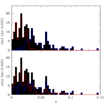
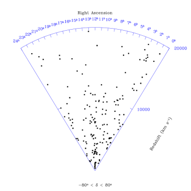
Figure 1: $Upper~{}Left~{}Panel$: The redshift distribution of HL AGN ($blue$) and LL AGN ($red$) overlaid to the full sample ($black$). $Bottom~{}Left~{}Panel$: The redshift distribution of Type I AGN ($blue$) and Type II AGN ($red$) overlaid to the full sample ($black$). $Right~{}Panel:$ A representation of the spatial distribution of local AGN with a redshift cone diagram of the Swift)-BAT AGN in the declination interval -80$<\delta<$80.

The sample used in this work consists of 199 non-blazar AGN detected by BAT during the first three years and precisely between March 2005 and March 2008. This sample is part of the one used in Ajello et al. (2009) which comprises all sources detected by BAT at high ($|$b$|$$>$15^∘) Galactic latitude and with a signal-to-noise ratio (S/N) exceeding 5 $\sigma$. The reader is referred to Ajello et al. (2009) for more details about the sample and the detection procedure. The flux limit at each direction in the sky has been computed, following Ajello et al. (2008), analyzing the local background around that position. For each source we use the redshift already provided in Ajello et al. (2009) and the measurement of the absorbing column density as determined from joint XMM-Newton/XRT–BAT fits (Burlon et al, in preparation). The redshift distribution of the sample is shown in Fig. 1 together with the redshift cone diagram of the survey up to 20000 km/s (z$\sim$0.07).

3 The two-point spatial auto-correlation function

The two-point auto-correlation function ($\xi(r)$, ACF) describes the excess probability over random of finding a pair with an object in the volume $dV_{1}$ and another in the volume $dV_{2}$, separated by a distance $r$ so that $dP=n^{2}[1+\xi(r)]dV_{1}dV_{2}$, where n is the mean space density. A known effect when measuring pairs separations is that the peculiar velocities combined with the Hubble flow may cause a biased estimate of the distance when using the spectroscopic redshift. To avoid this effect we computed the projected ACF (Davies & Peebles 1983): $w(r_{p})=2\int_{0}^{\pi_{max}}\xi(r_{p},\pi)d\pi$. Where $r_{p}$ is the distance component perpendicular to the line of sight and $\pi$ parallel to the line of sight (Fisher et al. 1994). It can be demonstrated that, if the ACF is expressed as $\xi(r)=(r/r_{0})^{-\gamma}$, then

$$w(r_{\rm p})=A(\gamma)r_{0}^{\gamma}r_{p}^{1-\gamma},$$ (1)

where $A(\gamma)=\Gamma(1/2)\Gamma[(\gamma-1)/2]/\Gamma(\gamma/2)$ (Peebles 1980).
The ACF has been estimated by using the minimum variance estimator described by Landy & Szalay (1993):

$$\xi(r_{p},\pi)=\frac{DD-2DR+RR}{RR}$$ (2)

where DD, DR and RR are the normalized number of data-data, data-random, and random-random source pairs, respectively. Equation 2 indicates that an accurate estimate of the distribution function of the random samples is crucial in order to obtain a reliable estimate of $\xi(r_{p},\pi)$. Several observational biases must be taken into account when generating a random sample of objects in a flux limited survey. In particular, in order to reproduce the selection function of the survey, one has to carefully reproduce the space and flux distributions of the sources, since the sensitivity of the survey in not homogeneous on the sky. Simulated AGN were randomly placed on the survey area. In order to reproduce the flux distribution of the real sample, we followed the method described in Mullis et al. (2004). The cumulative AGN logN-logS source count distribution, in the 15-55 keV band, can be described by a power law, $S=kS^{-\alpha}$, with $\alpha\sim 1.55$ (Ajello et al. 2008) Therefore, the differential probability scales as $S^{-(\alpha+1)}$. Using a transformation method the random flux above a certain X-ray flux $S_{lim}$ is distributed as $S=S_{lim}(1-p)^{\frac{-1}{\alpha}}$, where $p$ is a random number uniformly distributed between 0 and 1 and $S_{lim}$=7.6$\times 10^{-12}$ erg cm^-2 s^-1. All random AGN with a flux lower than the flux limit map at the source position were excluded. Redshift were randomly drawn from the smoothing of the real redshift distribution with a gaussian kernel with $\sigma_{z}$=0.3. An important choice for obtaining a reliable estimate of $w(r_{\rm p})$, is to set $\pi_{max}$ in the calculation of the integral above. One should avoid values of $\pi_{max}$ too large since they would add noise to the estimate of $w(r_{\rm p})$. If, instead, $\pi_{max}$ is too small one could not recover all the signal. We have calculated $w(r_{\rm p})$ by varying $\pi_{max}$ and found that the result converges at $\pi_{max}\sim$60 Mpc/h.
Errors on $w(r_{\rm p})$ were computed with a bootstrap resampling technique with 100 realizations. It is worth noting that in the literature, several methods are adopted for errors estimates in two-point statistics, and no one has been proved to be the most precise. However, it is known that Poisson estimators generally underestimate the variance because they do consider that points in ACF are not statistically independent. Jackknife resmpling method, where one divides the survey area in many sub fields and iteratively re-computes correlation functions by excluding one sub-field at a time, generally gives a good estimates of errors. But it requires that sufficient number of almost statistically independent sub-fields. This is not the case for our small sample. For these reasons we used the bootstrap resampling for the error estimate which, in our case, are comparable with the Poisson errors.

4 Results

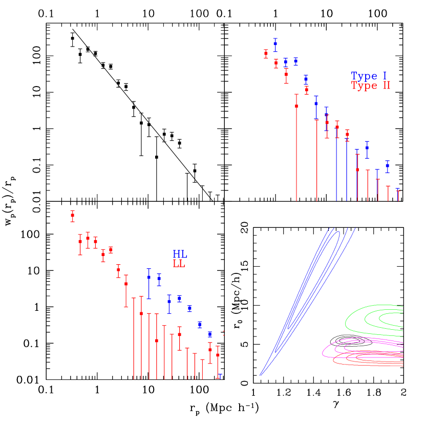
Figure 2: $Upper~{}Left~{}Panel:$ $w(r_{\rm p})/r_{p}$ for the whole sample, the solid line represents the best fit power-law. $Upper~{}Right~{}Panel:$ The ACF of type I AGN ($blue$) and Type II ($red$). $Bottom~{}Left~{}Panel:$ The ACF of HL ($blue$) and LL ($red$) AGN. $Bottom~{}Right:$ Confidence contours of the two parameter fit to $\xi(r)$ for the whole sample ($black$), Type I AGN ($green$), type II AGN ($pink$), HL AGN ($blue$) and LL ($red$).

We show in Fig. 2 the projected ACF measured on the whole AGN sample of the survey. The ACF has been evaluated in the projected separation range $\sim$0.2 Mpc/h $<r_{p}<$ 200 Mpc/h and has been plotted in form of $w(r_{\rm p})/r_{p}$ in order to reproduce the slope of $\xi(r)$ (see above). The bin size for computing $w(r_{\rm p})$ has been set to $\Delta log(r_{p},\pi)$=0.15. We obtained an estimate of $w(r_{\rm p})/r_{p}$ with a significance of the order 4$\sigma$-5$\sigma$. In order to evaluate the power of the clustering signal we fitted $w(r_{\rm p})$ with $\chi^{2}$ minimization technique by using Eq.1 as a model with $r_{0}$ and $\gamma$ as free parameters. The correction due to the integral constraint (Peebles 1980) is estimated to be much smaller than the statistical uncertainties in our sample, and thus has not been made. As a result we obtained $r_{0}$=5.56${}^{+0.49}_{-0.43}$ Mpc/h and $\gamma$=1.64${}^{+0.07}_{0.08}$. The confidence contours of the fit are presented in Fig. 2. We also measured the ACF for different data subsamples. We first divided the sample according to the column density: we defined as Type II AGN (or absorbed) sources with log$(N_{H})\geq$22 cm^-2 and as Type I AGN (or unabsorbed) sources if log$(N_{H})<$22 cm^-2. As a result we constructed a sample of 96 Type I AGN and one of 103 Type II AGN. For both samples we computed the ACF with the technique described above. We also split the sample into high and low luminosity subsamples. All the sources with L${}_{15-55}>$43.2 erg/s (i.e. the median luminosity of the whole sample, HL sources) were classified as high luminous, while the sources with L${}_{15-55}<$43.2 erg/s (LL sources) as low luminosity sources. The results of the measurement of the ACF as a function of the source type and luminosity class are presented in Fig. 2 together with the fit confidence contours. Note that for the HL sample the fit parameters are poorly constrained because of the lack of close pairs in the sample. We also repeated the fit by freezing $\gamma$ to 1.7, and obtained consistent results (Table 1). A summary of the fit results of all the samples used here is given in Table 1. Type I AGN show a larger correlation with respect to that of type II AGN, the significance of this difference is of the order $\sim 2.7\sigma-3.3\sigma$. HL AGN show a 1.7-4.6$\sigma$ higher correlation length with respect to LL AGN. We also checked the correlation between r₀ and $<L_{X}>$ of all the subsamples and found a linear correlation coefficient R=0.95, which corresponds to a $\sim 2\sigma$ significant correlation. We can use the weighted mean dispersion of the results on the measurement of r₀ in our subsamples to estimate the impact of sample variance on our results under the assumption that this is the main reason of the fluctuations. Our estimates suggest that overall our results are affected by this effect at $\sim$10% level. It is worth to note that our results are more significant than those obtained by e.g. Mullis et al. (2004), with a similar number of sources. This is because our sources are distributed in a much smaller volume than that sampled by the NEP survey and, by being on average less luminous, have an intrinsic higher space density resulting in a larger number of close source pairs.

Table 1: Summary of the results.

Sample	Na	$<z>$	$<log(L_{X})>$	r0	$\gamma$	r${}_{0_{\gamma=1.7}}^{b}$
			erg/s	Mpc/h		Mpc/h
All	199	0.045	43.2	5.56${}^{+0.49}_{-0.43}$	1.64${}_{-0.08}^{+0.07}$	5.54${}^{+0.1}_{-0.1}$
Type I	96	0.046	43.37	7.93${}^{+1.14}_{-0.79}$	2.1${}^{+0.20}_{-0.25}$	8.12${}_{-1.00}^{+1.57}$
Type II	103	0.024	42.87	4.72${}^{+0.60}_{-0.70}$	1.78${}^{+0.24}_{-0.17}$	4.90${}^{-0.70}_{+0.20}$
HL	99	0.054	43.67	13.92${}^{+5.48}_{-6.69}$	1.41${}^{+0.15}_{-0.19}$	15.63${}_{-2.57}^{+1.57}$
LL	100	0.023	42.55	3.37${}^{+0.51}_{-0.68}$	1.86${}^{+0.25}_{-0.17}$	3.56${}_{-0.66}^{+0.15}$

Table 2: Bias factor and Mass of the Dark matter halos hosts of the AGN in the samples.

Sample	b${}_{X}^{a}$	M${}_{DM}^{b}$	$\tau_{AGN}^{c}$	log(M${}_{BH})^{d}$)	log($\epsilon$)e	M∗f
		log(M/ h-1M⊙)	Gyr	log(M/M⊙)		1010/M⊙
All	$1.21^{+0.06}_{-0.07}$	$13.15^{+0.09}_{-0.13}$	0.68	8.51	-1.96	18.2
Type I	$2.01^{+0.15}_{-0.13}$	$13.94^{+0.15}_{-0.21}$	4.99	8.79	-2.02	31.6
Type II	$1.08^{+0.26}_{-0.29}$	$12.92^{+0.11}_{-0.38}$	1.32	7.96	-1.85	6.38
HL	$2.28^{+0.95}_{-0.90}$	$14.08^{+0.37}_{-0.70}$	3.91	9.28	-2.12	80.5
LL	$0.80^{+0.06}_{-0.16}$	$11.89^{+0.34}_{-\infty}$	0.24	7.43	-1.68	2.28

In the linear theory of structure formation, the bias factor defines the relation between the autocorrelation function of large scale structure tracers and the underlying overall matter distribution. In the case of X-ray selected AGN, we can define the following relation: $\xi_{X}(r,z)=b_{X}(r,z)^{2}\xi_{m}(r,z)$, where $\xi_{X}$, $\xi_{m}$ and b_X are the autocorrelation function of AGN, of DM and the AGN bias factor, respectively. In order to compute the b_X, we estimated the amplitude of the fluctuations of the AGN distribution in a sphere of 8 Mpc/h (also know as $\sigma_{8}$), by using Eq. 12 and 13 of Miyaji et al. (2007) and all the combinations of r₀ and $\gamma$ are reported in Tab. 1. In order to derive the bias factor of the AGN in our samples we used $b_{AGN}=\sigma_{\rm 8,AGN}(z)/\sigma_{8}D(z)$, where D(z) is the growth factor. This quantity allows us to compare the observed AGN clustering to the underlying mass distribution from linear growth theory (Hamilton 2001). As a result we obtain for the whole sample b_AGN(z$\sim$0.04)=1.21${}^{+0.06}_{-0.07}$. We have repeated this calculation for all the samples listed in Table 1 and we report the corresponding values of the bias factor in Table 2, for all the possible best fit results.
It is widely accepted that the clustering amplitude of DMH depends primarily on their mass (see e.g. Sheth et al. 2001). In this way, we can estimate the typical mass of the DMH in which the population of AGN reside, under the assumption that the typical mass of the host halo is the only variable that causes AGN biasing. We have then computed the expected large-scale bias factor for different dark matter halo masses by using the prescription of Tinker et al. (2005). The required ratio of the critical overdensity to the rms fluctuation on a given size and mass is calculated by $\nu=\delta_{\rm cr}/\sigma(M,z)$, for our purposes we assumed $\delta_{\rm cr}\approx 1.69$ and compute $\sigma_{8}(M,z)$ and therefore $b(M,z)$ using Eq. A8, A9, and A10 in van den Bosch (2002). The typical DMH mass that hosts an AGN has been estimated to be $log(M_{DMH})$=13.15${}^{+0.09}_{-0.13}$ h^-1M/M_⊙. This is consistent with similar measurements in the local Universe of Krumpe et al. (2010), Grazian et al. (2004) and Akilas et al. (2000). We have computed the typical mass of the DMH for all the subsamples listed in Table 1 and reported for simplicity in Table 2. Following Martini & Weinberg(2001), by knowing the AGN and DMH halo space density at a given luminosity and mass ($n_{AGN},n_{DMH}$), one can estimate the duty cycle of the AGN, $\tau_{AGN}(z)=\frac{n_{AGN}(L,z)}{n_{DMH}(M,z)}\tau_{H}(z)$. Where $\tau_{H}(z)$ is the Hubble time at a given redshift. For the whole sample at z$\sim$0, $n_{DMH}\sim$6.7$\times$10^-4 Mpc^-3 (Hamana et al. 2002) and $n_{AGN}\sim$3.4$\times$10^-5 Mpc^-3 (Sazonov et al. 2007) which leads to an estimate of $\tau_{AGN}(z=0)\sim$0.68 Gyr. To fully characterize our sample, we derived the average properties of the active BHs and their host galaxies. By using the bolometric correction prescribed by Hopkins et al. (2007) we estimated from $<L_{X}>$, $<L_{Bol}>$ and $<L_{B}>$ (B band luminosity). L_B is related to the black holes mass and the stellar mass of the host galaxy via scaling relations (Marconi & Hunt 2003). From $<M_{BH}>$ we derived $<L_{Edd}>$ and the Eddington rate $\epsilon$=$<L_{Bol}>/<L_{Edd}>$ (see Table 2 for a summary). We point out that the estimates obtained above have several limitations which mostly arise from the uncertainties on scaling relations and from the broad range of luminosities sampled here. We therefore consider these values as estimate for the “average” local AGN population.

5 Summary and discussion

In this letter we report on the measurement of clustering of 199 AGN in the local Universe using the Swift/BAT all-sky survey sample. This result gives, for the first time, an unbiased picture of the z=0 DMH-galaxy-AGN coexistence/evolution. We obtained a correlation length r₀=5.56${}^{+0.49}_{-0.43}$ Mpc/h and $\gamma$=1.64${}_{-0.08}^{+0.07}$. We measured the ACF for Type I and Type II AGN and found a significant difference in their correlation lengths. We have measured a marginally significant higher r₀ for high luminosity AGN than for the low luminosity ones. We propose that the observed difference in Type I vs. Type II clustering is driven by the intrinsic higher $<L_{X}>$ of Type I AGN as we show a marginal evidence of a correlation between r₀ and $L_{X}$. We estimated the typical mass of the DMH hosting an AGN of the order log(M_MDH)$\sim$13.15 h^-1M/M_⊙. In Fig. 3 we show the bias-redshift plane results from AGN and galaxy surveys (references in the figure). In the same plot we show the expected evolution of different DMH masses. We compared only bias values of studies that rely on the real space correlation function $\xi(r)$ (values of $\sigma_{\rm 8,AGN/GAL}$ from Krumpe et al. 2010). This approach allows us to compare all different clustering studies on a common basis.

The majority of the X-ray surveys agree with a picture where AGN are typically hosted in DM halos with mass of the order of 12.5 h^-1M/M${}_{\odot}<$ log(M_MDH)$<$13.5 h^-1M/M_⊙ which is the mass of moderately poor group. Optically selected AGN instead reside in lower density environment and of the order of the log(M_MDH)$\sim$12.5 h^-1M/M_⊙. Another interesting aspect is that X-ray selected AGN samples (including ours) cluster similarly to red galaxies and that LL AGN or type II AGN are found typically in less massive environments. On the contrary HL AGN and Type I AGN are hosted in massive galaxies in massive DM halos (clusters).

We estimated that Swift-BAT AGN are powered by black holes with a typical  mass log(M${}_{BH}/M_{\odot}$) $\sim$8.5, accreting at very low Eddington ratio (i.e. $\sim$0.01 L_Edd) and that they are hosted by massive galaxies with mass of the order $\sim 2\times 10^{11}$ M/M_⊙. These properties, except $\epsilon$, scale with $<L_{X}>$ and Type (HL and Type I are hosted in higher mass DMH in more massive galaxies with bigger black holes). The upper limits on the duty cycle suggest that these AGN are shining since at least for 0.2-1.2 Gyr .

We then tested the AGN merger-driven triggering paradigm by comparing the theoretical predictions for AGN clustering of the model of Marulli et al. (2008) and Bonoli et al. (2009) with our results on the whole sample. The theoretical model is based on the assumption that AGN activity is triggered by galaxy mergers and the lightcurve associated to each accretion event is described by an Eddington-limited phase followed by a quiescent phase modeled after Hopkins et al. (2005). Applied to the Millennium Simulation (Springel et al. 2005), such model has been shown to be successful in reproducing the main properties of the black hole and AGN populations (Marulli et al. 2008) and the clustering of optical quasars (Bonoli et al. 2009). Using this model, we computed the expected correlation length of a sample of simulated AGN at z$\sim$0 with intrinsic $L_{bol}$ luminosities similar to the ones of our observed AGN. The model predicts a clustering length r₀=5.68$\pm{0.08}$ which is in agreement within 1$\sigma$ with our measurement.

By merging the observational evidences and the model predictions, a plausible scenario for the history of local AGN is the following:

• Swift-BAT AGN switched on about 0.7 Gyr Ago after a galaxy merger event.

• They shine in an Eddington-limited regime for the first part of their lives where they gain most of their mass.

• In the second phase of their lives (i.e. after 0.2-0.5 Gyr) they start to accrete with lower and lower efficiency. Their luminosity drops because of the decreased gas reservoirs.

• At z$\sim$0 they have grown to $\sim$10^8-9 M$/M_{\odot}$ SMBHs, shining as moderately low-luminosity AGN at low accretion rates.

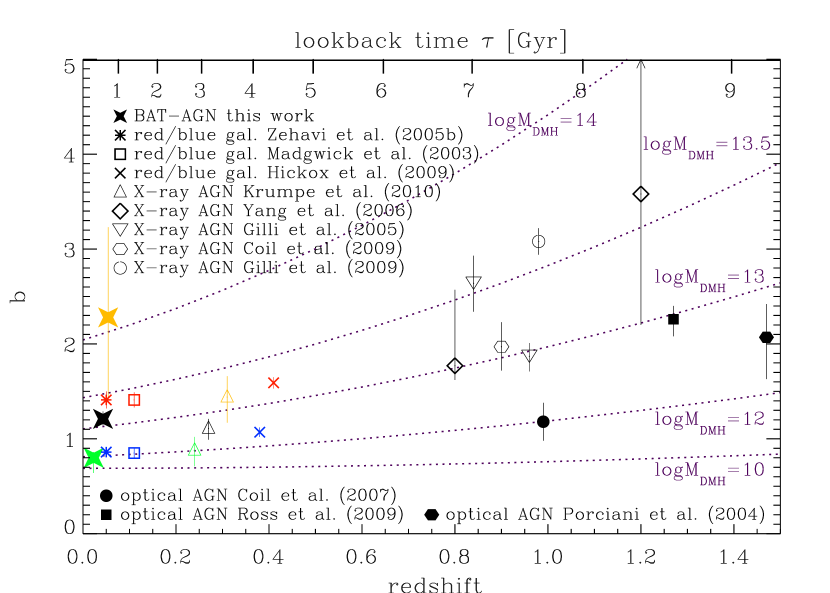
Figure 3: Bias parameter $b_{\rm AGN}$ as a function of redshift for studies that are based on the real space correlation function. Yellow (green) symbols represent high (low)luminosity subsamples of the corresponding study. The blue points for galaxy clustering measurements belong to blue galaxies, while red points represent the red galaxy sample. The dotted lines give the expected $b(z)$ of typical dark matter halo masses based on Sheth et al. (2001) and van den Bosch (2002). The masses are given in log $M_{\rm DMH}$ in units of $h^{-1}$ $M_{\odot}$.

References

- Ajello et al. (2008) Ajello, M., et al. 2008, ApJ, 673, 96
- Ajello et al. (2009) Ajello, M., et al. 2009, ApJ, 699, 603
- Barthelmy et al. (2005) Barthelmy, S. D., et al. 2005, Space Science Reviews, 120, 143
- Bonoli et al. (2009) Bonoli, S., Marulli, F., Springel, V., White, S. D. M., Branchini, E., & Moscardini, L. 2009, MNRAS, 396, 423
- Coil et al. (2009) Coil, A.L., Georgakakis, A., Newman, J.A., et al. 2009, ApJ, 701, 1484
- Davis & Peebles (1993) Davis, M., & Peebles, P. J. E. 1983, ApJ, 267, 465
- Gilli et al. (2009) Gilli, R., Zamorani, G., Miyaji, T., et al. 2009, A&A, 494, 33
- Gehrels et al. (2004) Gehrels, N., et al. 2004, ApJ, 611, 1005
- Grazian et al. (2004) Grazian, A., Negrello, M., Moscardini, L., Cristiani, S., Haehnelt, M. G., Matarrese, S., Omizzolo, A., & Vanzella, E. 2004, AJ, 127, 592
- Hamana et al. (2002) Hamana, T., Yoshida, N., & Suto, Y. 2002, ApJ, 568, 455
- Hamilton (2001) Hamilton, A.J.S., 2001, MNRAS, 322, 419
- Hasinger (2008) Hasinger, G., 2008, A&A, 490, 905
- Häring, N. & Rix (2004) Häring, N., & Rix, H.-W. 2004, ApJ, 604, L89
- Hickox et al. (2009) Hickox, R.C., Jones, C., Forman, W.R., et al, 2009, ApJ, 696, 891
- Hopkins et al. (2005) Hopkins, P. F., Hernquist, L., Martini, P., Cox, T. J., Robertson, B., Di Matteo, T., & Springel, V. 2005, ApJ, 625, L71
- Hopkins et al. (2007) Hopkins, P. F., Lidz, A., Hernquist, L., Coil, A. L., Myers, A. D., Cox, T. J., & Spergel, D. N. 2007, ApJ, 662, 110
- Kormendy et al. (1995) Kormendy, J., & Richstone, D. 1995, ARA&A, 33, 581
- Krumpe et al. (2010) Krumpe, M., Miyaji, T., & Coil, A. L. 2010, ApJ, 713, 558
- Landy & Szalay (1993) Landy, S. D., & Szalay, A. S. 1993, ApJ, 412, 64
- Magorrian et al. (1998) Magorrian, J., et al. 1998, AJ, 115, 2285
- Martini et al. (2001) Martini, P., & Weinberg, D. H. 2001, ApJ, 547, 12
- Marulli et al. (2008) Marulli, F., Bonoli, S., Branchini, E., Moscardini, L., & Springel, V. 2008, MNRAS, 385, 1846
- Miyaji et al. (2007) Miyaji, T., et al. 2007, ApJS, 172, 396
- Peebles (1980) Peebles, P. J. E. 1980, The large-scale structure of the universe (Princeton, N.J., Princeton University Press)
- Sazonov et al. (2007) Sazonov, S., Revnivtsev, M., Krivonos, R., Churazov, E., & Sunyaev, R. 2007, A&A, 462, 57
- Sheth et al. (2001) Sheth, R.K., Mo, H.J., Tormen, G., MNRAS, 323, 1
- Springel et al. (2005) Springel, V., et al. 2005, Nature, 435, 629
- Tueller et al. (2009) Tueller, J., et al. 2009, arXiv:0903.3037
- van den Bosch et al. (2002) van den Bosch, F.C., 2002,MNRAS, 331, 98
- Yang et al. (2006) Yang, Y., Mushotzky, R.F., Barger, A.J., Cowie, L.L. 2006, 645,68