Smoothing proximal gradient method for general structured sparse regression

Abstract

We study the problem of estimating high-dimensional regression models regularized by a structured sparsity-inducing penalty that encodes prior structural information on either the input or output variables. We consider two widely adopted types of penalties of this kind as motivating examples: (1) the general overlapping-group-lasso penalty, generalized from the group-lasso penalty; and (2) the graph-guided-fused-lasso penalty, generalized from the fused-lasso penalty. For both types of penalties, due to their nonseparability and nonsmoothness, developing an efficient optimization method remains a challenging problem. In this paper we propose a general optimization approach, the smoothing proximal gradient (SPG) method, which can solve structured sparse regression problems with any smooth convex loss under a wide spectrum of structured sparsity-inducing penalties. Our approach combines a smoothing technique with an effective proximal gradient method. It achieves a convergence rate significantly faster than the standard first-order methods, subgradient methods, and is much more scalable than the most widely used interior-point methods. The efficiency and scalability of our method are demonstrated on both simulation experiments and real genetic data sets.

, , , and

t1Supported by Grants ONR N000140910758, NSF DBI-0640543, NSF CCF-0523757, NIH 1R01GM087694, AFOSR FA95501010247, NIH 1R01GM093156 and an Alfred P. Sloan Research Fellowship awarded to EPX.

1 Introduction

The problem of high-dimensional sparse feature learning arises in many areas in science and engineering. In a typical setting such as linear regression, the input signal leading to a response (i.e., the output) lies in a high-dimensional space, and one is interested in selecting a small number of truly relevant variables in the input that influence the output. A popular approach to achieve this goal is to jointly optimize the fitness loss function with a nonsmooth $\ell_{1}$-norm penalty, for example, Lasso [Tibshirani (1996)] that shrinks the coefficients of the irrelevant input variables to zero. However, this approach is limited in that it is incapable of capturing any structural information among the input variables. Recently, various extensions of the $\ell_{1}$-norm lasso penalty have been introduced to take advantage of the prior knowledge of the structures among inputs to encourage closely related inputs to be selected jointly [Jenatton, Audibert and Bach (2009), Tibshirani and Saunders (2005), Yuan and Lin (2006)]. Similar ideas have also been explored to leverage the output structures in multivariate-response regression (or multi-task regression), where one is interested in estimating multiple related functional mappings from a common input space to multiple outputs [Kim and Xing (2009, 2010), Obozinski, Taskar and Jordan (2009)]. In this case, the structure over the outputs is available as prior knowledge, and the closely related outputs according to this structure are encouraged to share a similar set of relevant inputs. These progresses notwithstanding, the development of efficient optimization methods for solving the estimation problems resultant from the structured sparsity-inducing penalty functions remains a challenge for reasons we will discuss below. In this paper we address the problem of developing efficient optimization methods that can handle a broad family of structured sparsity-inducing penalties with complex structures.

When the structure to be imposed during shrinkage has a relatively simple form, such as nonoverlapping groups over variables (e.g., group lasso [Yuan and Lin (2006)]) or a linear-ordering (a.k.a., chain) of variables (e.g., fused lasso [Tibshirani and Saunders (2005)]), efficient optimization methods have been developed. For example, under group lasso, due to the separability among groups, a proximal operator associated with the penalty can be computed in closed-form; thus, a number of composite gradient methods [Beck and Teboulle (2009), Liu, Ji and Ye (2009), Nesterov (2007)] that leverage the proximal operator as a key step (so-called “proximal gradient method”) can be directly applied. For fused lasso, although the penalty is not separable, a coordinate descent algorithm was shown feasible by explicitly leveraging the linear ordering of the inputs [Friedman et al. (2007)].

Unfortunately, these algorithmic advancements have been outpaced by the emergence of more complex structures one would like to impose during shrinkage. For example, in order to handle a more general class of structures such as a tree or a graph over variables, various regression models that further extend the group lasso and fused lasso ideas have been recently proposed. Specifically, rather than assuming the variable groups to be nonoverlapping as in the standard group lasso, the overlapping group lasso [Jenatton, Audibert and Bach (2009)] allows each input variable to belong to multiple groups, thereby introducing overlaps among groups and enabling incorporation of more complex prior knowledge on the structure. Going beyond the standard fused lasso, the graph-guided fused lasso extends the original chain structure over variables to a general graph over variables, where the fused-lasso penalty is applied to each edge of the graph [Kim, Sohn and Xing (2009)]. Due to the nonseparability of the penalty terms resultant from the overlapping group or graph structures in these new models, the aforementioned fast optimization methods originally tailored for the standard group lasso or fused lasso cannot be readily applied here, due to, for example, unavailability of a closed-form solution of the proximal operator. In principle, generic convex optimization solvers such as the interior-point methods (IPM) could always be used to solve either a second-order cone programming (SOCP) or a quadratic programming (QP) formulation of the aforementioned problems; but such approaches are computationally prohibitive for problems of even a moderate size. Very recently, a great deal of attention has been given to devise practical solutions to the complex structured sparse regression problems discussed above in statistics and the machine learning community, and numerous methods have been proposed [Duchi and Singer (2009), Jenatton et al. (2010), Liu, Yuan and Ye (2010), Mairal et al. (2010), Tibshirani and Taylor (2010), Zhou and Lange (2011)]. All of these recent works strived to provide clever solutions to various subclasses of the structured sparsity-inducing penalties; but, as we survey in Section 4, they are still short of reaching a simple, unified and general solution to a broad class of structured sparse regression problems.

In this paper we propose a generic optimization approach, the smoothing proximal gradient (SPG) method, for dealing with a broad family of sparsity-inducing penalties of complex structures. We use the overlapping-group-lasso penalty and graph-guided-fused-lasso penalty mentioned above as our motivating examples. Although these two types of penalties are seemingly very different, we show that it is possible to decouple the nonseparable terms in both penalties via the dual norm; and reformulate them into a common form to which the proposed method can be applied. We call our approach a “smoothing” proximal gradient method because instead of optimizing the original objective function directly as in other proximal gradient methods, we introduce a smooth approximation to the structured sparsity-inducing penalty using the technique from Nesterov (2005). Then, we solve the smoothed surrogate problem by a first-order proximal gradient method known as the fast iterative shrinkage-thresholding algorithm (FISTA) [Beck and Teboulle (2009)]. We show that although we solve a smoothed problem, when the smoothness parameter is carefully chosen, SPG achieves a convergence rate of $O(\frac{1}{\varepsilon})$ for the original objective for any desired accuracy $\varepsilon$. Below, we summarize the main advantages of this approach:

[(a)]

It is a first-order method, as it uses only the gradient information. Thus, it is significantly more scalable than IPM for SOCP or QP. Since it is gradient-based, it allows warm restarts, and thereby potentiates solving the problem along the entire regularization path [Friedman et al. (2007)].

It is applicable to a wide class of optimization problems with a smooth convex loss and a nonsmooth nonseparable structured sparsity-inducing penalty. Additionally, it is applicable to both uni- and multi-task sparse structured regression, with structures on either (or both) inputs/outputs.

Theoretically, it enjoys a convergence rate of $O(\frac{1}{\varepsilon})$, which dominates that of the standard first-order method such as the subgradient method whose rate is of $O(\frac{1}{\varepsilon^{2}})$.

Finally, SPG is easy to implement with a few lines of MATLAB code.

The idea of constructing a smoothing approximation to a difficult-to-optimize objective function has also been adopted in another widely used optimization framework known as majorization–minimization (MM) [Lange (2004)]. Using the quadratic surrogate functions for the $\ell_{2}$-norm and fused-lasso penalty as derived in Wu and Lange (2008) and Zhang et al. (2010), one can also apply MM to solve the structured sparse regression problems. We will discuss in detail the connections between our methods and MM in Section 4.

The rest of this paper is organized as follows. In Section 2 we present the formulation of overlapping group lasso and graph-guided fused lasso. In Section 3 we present the SPG method along with complexity results. In Section 4 we discuss the connections between our method and MM, and comparisons with other related methods. In Section 5 we extend our algorithm to multivariate-task regression. In Section 6 we present numerical results on both simulated and real data sets, followed by conclusions in Section 7. Throughout the paper, we will discuss overlapping-group-lasso and graph-guided-fused-lasso penalties in parallel to illustrate how the SPG can be used to solve the corresponding optimization problems generically.

2 Background: Linear regression regularized by structured sparsity-inducing penalties

We begin with a basic outline of the high-dimensional linear regression model, regularized by structured sparsity-inducing penalties.

Consider a data set of $N$ feature/response (i.e., input/output) pairs, $\{{\mathbf{x}}_{n},y_{n}\}$, $n=1,\ldots,N$. Let ${\mathbf{X}}\in\mathbb{R}^{N\times J}$ denote the matrix of inputs of the $N$ samples, where each sample lies in a $J$-dimensional space; and ${\mathbf{y}}\in\mathbb{R}^{N\times 1}$ denote the vector of univariate outputs of the $N$ sample. Under a linear regression model, ${\mathbf{y}}={\mathbf{X}}{\bolds\beta}+{\bolds\varepsilon},$ where ${\bolds\beta}$ represents the vector of length $J$ for the regression coefficients, and ${\bolds\varepsilon}$ is the vector of length $N$ for noise distributed as $N(0,\sigma^{2}I_{N\times N})$. The well-known Lasso regression [Tibshirani (1996)] obtains a sparse estimate of the coefficients by solving the following optimization problem:

$$\min_{{\bolds\beta}\in\mathbb{R}^{J}}g({\bolds\beta})+\lambda\|{\bolds\beta}\|_{1},$$ (1)

where $g({\bolds\beta})\equiv\frac{1}{2}\|{\mathbf{y}}-{\mathbf{X}}{\bolds\beta}\|_{2}^{2}$ is the squared-error loss, $\|{\bolds\beta}\|_{1}\equiv{\sum_{j=1}^{J}}|\beta_{j}|$ is the $\ell_{1}$-norm penalty that encourages the solutions to be sparse, and $\lambda$ is the regularization parameter that controls the sparsity level.

The standard lasso penalty does not assume any structure among the input variables, which limits its applicability to complex high-dimensional scenarios in many applied problems. More structured constraints on the input variables such as groupness or pairwise similarities can be introduced by employing a more sophisticated sparsity-inducing penalty that induces joint sparsity patterns among related inputs. We generically denote the structured sparsity-inducing penalty by $\Omega({\bolds\beta})$ without assuming a specific form, and define the problem of estimating a structured sparsity pattern of the coefficients as follows:

$$\min_{{\bolds\beta}\in\mathbb{R}^{J}}f({\bolds\beta})\equiv g({\bolds\beta})+\Omega({\bolds\beta})+\lambda\|{\bolds\beta}\|_{1}.$$ (2)

In this paper we consider two types of $\Omega({\bolds\beta})$ that capture two different kinds of structural constraints over variables, namely, the overlapping-group-lasso penalty based on the $\ell_{1}/\ell_{2}$ mixed-norm, and the graph-guided-fused-lasso penalty based on a total variation norm. As we discuss below, these two types of penalties represent a broad family of structured sparsity-inducing penalties recently introduced in the literature [Jenatton, Audibert and Bach (2009), Kim and Xing (2010), Kim, Sohn and Xing (2009), Tibshirani and Saunders (2005), Yuan and Lin (2006), Zhao, Rocha and Yu (2009a)]. It is noteworthy that in problem (2), in addition to the structured-sparsity-inducing penalty $\Omega({\bolds\beta})$, there is also an $\ell_{1}$-regularizer $\lambda\|{\bolds\beta}\|_{1}$ that explicitly enforces sparsity on every individual feature. The SPG optimization algorithm to be presented in this paper is applicable regardless of the presence or absence of the $\lambda\|{\bolds\beta}\|_{1}$ term.

[(2)]

Overlapping-group-lasso penalty. Given prior knowledge of (possibly overlapping) grouping of variables or features, if it is desirable to encourage coefficients of features within the same group to be shrunk to zero jointly, then a composite structured penalty of the following form can be used:

$$\Omega({\bolds\beta})\equiv\gamma\sum_{g\in\mathcal{G}}w_{g}\|{\bolds\beta}_{g}\|_{2},$$ (3)

where $\mathcal{G}=\{g_{1},\ldots,g_{|\mathcal{G}|}\}$ denotes the set of groups, which is a subset of the power set of $\{1,\ldots,J\}$; ${\bolds\beta}_{g}\in\mathbb{R}^{|g|}$ is the subvector of ${\bolds\beta}$ for the features in group $g$; $w_{g}$ is the predefined weight for group $g$; and $\|\cdot\|_{2}$ is the vector $\ell_{2}$-norm. This $\ell_{1}/\ell_{2}$ mixed-norm penalty plays the role of jointly setting all of the coefficients within each group to zero or nonzero values. The widely used hierarchical tree-structured penalty [Kim and Xing (2010), Zhao, Rocha and Yu (2009b)] is a special case of (3), of which the groups are defined as a nested set under a tree hierarchy. It is noteworthy that the $\ell_{1}/\ell_{\infty}$ mixed-norm penalty can also achieve a similar grouping effect. Indeed, our approach can also be applied to the $\ell_{1}/\ell_{\infty}$ penalty, but for simplicity here we focus on only the $\ell_{1}/\ell_{2}$ penalty and the comparison between the $\ell_{1}/\ell_{2}$ and the $\ell_{1}/\ell_{\infty}$ is beyond the scope of the paper.

Apparently, the penalty $\Omega({\bolds\beta})\equiv\gamma\sum_{g\in\mathcal{G}}w_{g}\|{\bolds\beta}_{g}\|_{2}$ alone enforces only group-level sparsity but not sparsity within each group. More precisely, if the estimated $\|\widehat{{\bolds\beta}}_{g}\|_{2}\neq 0$, each $\widehat{\beta}_{j}$ for $j\in g$ will be nonzero. By using an additional $\ell_{1}$-regularizer $\lambda\|{\bolds\beta}\|_{1}$ together with $\Omega({\bolds\beta})$ as in (2), one cannot only select groups but also variables within each group. The readers may refer to Friedman, Hastie and Tibshirani (2010) for more details.

Graph-guided-fused-lasso penalty. Alternatively, prior knowledge about the structural constraints over features can be in the form of their pairwise relatedness described by a graph $G\equiv(V,E)$, where $V=\{1,\ldots,J\}$ denotes the variables or features of interest, and $E$ denotes the set of edges among $V$. Additionally, we let $r_{ml}\in\mathbb{R}$ denote the weight of the edge $e=(m,l)\in E$, corresponding to correlation or other proper similarity measures between features $m$ and $l$. If it is desirable to encourage coefficients of related features to share similar magnitude, then the graph-guided-fused-lasso penalty [Kim, Sohn and Xing (2009)] of the following form can be used:

$$\Omega({\bolds\beta})=\gamma\sum_{e=(m,l)\in E,m<l}\tau(r_{ml})|\beta_{m}-\operatorname{sign}(r_{ml})\beta_{l}|,$$ (4)

where $\tau(r_{ml})$ represent a general weight function that enforces a fusion effect over coefficients $\beta_{m}$ and $\beta_{l}$ of relevant features. In this paper we consider $\tau(r)=|r|$, but any monotonically increasing function of the absolute values of correlations can be used.

The $\operatorname{sign}(r_{ml})$ in (4) ensures that two positively correlated inputs would tend to influence the output in the same direction, whereas two negatively correlated inputs impose opposite effect. Since the fusion effect is calibrated by the edge weight, the graph-guided-fused-lasso penalty in (4) encourages highly inter-correlated inputs corresponding to a densely connected subnetwork in $G$ to be jointly selected as relevant.

It is noteworthy that when $r_{ml}=1$ for all $e=(m,l)\in E$, and $G$ is simply a chain over nodes, we have

$$\Omega({\bolds\beta})=\gamma\sum_{j=1}^{J-1}|\beta_{j+1}-\beta_{j}|,$$ (5)

which is identical to the standard fused lasso penalty [Tibshirani and Saunders (2005)].

3 Smoothing proximal gradient

Although (2) defines a convex program, of which a globally optimal solution to ${\bolds\beta}$ is attainable, the main difficulty in solving (2) arises from the nonseparability of elements of ${\bolds\beta}$ in the nonsmooth penalty function $\Omega({\bolds\beta})$. As we show in the next subsection, although the overlapping-group-lasso and graph-guided-fused-lasso penalties are seemingly very different, we can reformulate the two types of penalties as a common matrix algebraic form, to which a generic Nesterov smoothing technique can be applied. The key in our approach is to decouple the nonseparable structured sparsity-inducing penalties into a simple linear transformation of ${\bolds\beta}$ via the dual norm. Based on that, we introduce a smooth approximation to $\Omega({\bolds\beta})$ using the technique from Nesterov (2005) such that its gradient with respect to ${\bolds\beta}$ can be easily calculated.

3.1 Reformulation of structured sparsity-inducing penalty

In this section we show that utilizing the dual norm, the nonseparable structured sparsity-inducing penalty in both (3) and (4) can be decoupled; and reformulated into a common form as a maximization problem over the auxiliary variables.

[(1)]

Reformulating overlapping-group-lasso penalty. Since the dual norm of an $\ell_{2}$-norm is also $\ell_{2}$-norm, we can write $\|{\bolds\beta}_{g}\|_{2}$ as $\|{\bolds\beta}_{g}\|_{2}=\max_{\|{\bolds\alpha}_{g}\|_{2}\leq 1}{\bolds\alpha}_{g}^{T}{\bolds\beta}_{g}$, where ${\bolds\alpha}_{g}\in\mathbb{R}^{|g|}$ is a vector of auxiliary variables associated with ${\bolds\beta}_{g}$. Let ${\bolds\alpha}=[{\bolds\alpha}_{g_{1}}^{T},\ldots,{\bolds\alpha}_{g_{|\mathcal{G}|}}^{T}]^{T}$. Then, ${\bolds\alpha}$ is a vector of length $\sum_{g\in G}|g|$ with domain $\mathcal{Q}\equiv\{{\bolds\alpha}|\|{\bolds\alpha}_{g}\|_{2}\leq 1,\forall g\in\mathcal{G}\}$, where $\mathcal{Q}$ is the Cartesian product of unit balls in Euclidean space and, therefore, a closed and convex set. We can rewrite the overlapping-group-lasso penalty in (3) as

$$\quad\Omega({\bolds\beta})=\gamma\sum_{g\in\mathcal{G}}w_{g}\max_{\|{\bolds\alpha}_{g}\|_{2}\leq 1}{\bolds\alpha}_{g}^{T}{\bolds\beta}_{g}=\max_{{\bolds\alpha}\in\mathcal{Q}}\sum_{g\in\mathcal{G}}\gamma w_{g}{\bolds\alpha}_{g}^{T}{\bolds\beta}_{g}=\max_{{\bolds\alpha}\in\mathcal{Q}}{\bolds\alpha}^{T}C{\bolds\beta},$$ (6)

where $C\in\mathbb{R}^{{\sum_{g\in\mathcal{G}}|g|}\times J}$ is a matrix defined as follows. The rows of $C$ are indexed by all pairs of $(i,g)\in\{(i,g)|i\in g,i\in\{1,\ldots,J\},g\in\mathcal{G}\}$, the columns are indexed by $j\in\{1,\ldots,J\}$, and each element of $C$ is given as

$$C_{(i,g),j}=\cases{\gamma w_{g},&\quad if $i=j$,\cr 0,&\quad otherwise.}$$ (7)

Note that $C$ is a highly sparse matrix with only a single nonzero element in each row and $\sum_{g\in\mathcal{G}}|g|$ nonzero elements in the entire matrix, and, hence, can be stored with only a small amount of memory during the optimization procedure.

Reformulating graph-guided-fused-lasso penalty. First, we rewrite the graph-guided-fused-lasso penalty in (4) as follows:

$$\gamma\sum_{e=(m,l)\in E,m<l}\tau(r_{ml})|\beta_{m}-\operatorname{sign}(r_{ml})\beta_{l}|\equiv\|C{\bolds\beta}\|_{1},$$

where $C\in\mathbb{R}^{|E|\times J}$ is the edge-vertex incident matrix:

$$C_{e=(m,l),j}=\cases{\gamma\cdot\tau(r_{ml}),&\quad if $j=m$,\cr-\gamma\cdot\operatorname{sign}(r_{ml})\tau(r_{ml}),&\quad if $j=l$,\cr 0,&\quad otherwise.}$$ (8)

Again, we note that $C$ is a highly sparse matrix with $2\cdot|E|$ nonzero elements. Since the dual norm of the $\ell_{\infty}$-norm is the $\ell_{1}$-norm, we can further rewrite the graph-guided-fused-lasso penalty as

$$\|C{\bolds\beta}\|_{1}\equiv\max_{\|{\bolds\alpha}\|_{\infty}\leq 1}{\bolds\alpha}^{T}C{\bolds\beta},$$ (9)

where ${\bolds\alpha}\in\mathcal{Q}=\{{\bolds\alpha}|\|{\bolds\alpha}\|_{\infty}\leq 1,{\bolds\alpha}\in\mathbb{R}^{|E|}\}$ is a vector of auxiliary variables associated with $\|C{\bolds\beta}\|_{1}$, and $\|\cdot\|_{\infty}$ is the $\ell_{\infty}$-norm defined as the maximum absolute value of all entries in the vector.

Remark 1.

As a generalization of the graph-guided-fused-lasso penalty, the proposed optimization method can be applied to the $\ell_{1}$-norm of any linear mapping of ${\bolds\beta}$ [i.e., $\Omega({\bolds\beta})=\|C{\bolds\beta}\|_{1}$ for any given $C$].

3.2 Smooth approximation to structured sparsity-inducing penalty

The common formulation of $\Omega({\bolds\beta})$ given above [i.e., $\Omega({\bolds\beta})=\max_{{\bolds\alpha}\in\mathcal{Q}}{\bolds\alpha}^{T}C{\bolds\beta}$] is still a nonsmooth function of ${\bolds\beta}$, and this makes the optimization challenging. To tackle this problem, using the technique from Nesterov (2005), we construct a smooth approximation to $\Omega({\bolds\beta})$ as follows:

$$f_{\mu}({\bolds\beta})=\max_{{\bolds\alpha}\in\mathcal{Q}}\bigl{(}{\bolds\alpha}^{T}C{\bolds\beta}-\mu\,d({\bolds\alpha})\bigr{)},$$ (10)

where $\mu$ is a positive smoothness parameter and $d({\bolds\alpha})$ is a smoothing function defined as $\frac{1}{2}\|{\bolds\alpha}\|_{2}^{2}$. The original penalty term can be viewed as $f_{\mu}({\bolds\beta})$ with $\mu=0$; and one can verify that $f_{\mu}({\bolds\beta})$ is a lower bound of $f_{0}({\bolds\beta})$. In order to bound the gap between $f_{\mu}({\bolds\beta})$ and $f_{0}({\bolds\beta})$, let $D=\max_{{\bolds\alpha}\in\mathcal{Q}}d({\bolds\alpha})$. In our problems, $D=|\mathcal{G}|/2$ for the overlapping-group-lasso penalty and $D=|E|/2$ for the graph-guided-fused-lasso penalty. Then, it is easy to verify that the maximum gap between $f_{\mu}({\bolds\beta})$ and $f_{0}({\bolds\beta})$ is $\mu D$:

$$f_{0}({\bolds\beta})-\mu D\leq f_{\mu}({\bolds\beta})\leq f_{0}({\bolds\beta}).$$

From Theorem 1 as presented below, we know that $f_{\mu}({\bolds\beta})$ is a smooth function for any $\mu>0$. Therefore, $f_{\mu}({\bolds\beta})$ can be viewed as a smooth approximation to $f_{0}({\bolds\beta})$ with a maximum gap of $\mu D$; and the $\mu$ controls the gap between $f_{\mu}({\bolds\beta})$ and $f_{0}({\bolds\beta})$. Given a desired accuracy $\varepsilon$, the convergence result in Section 3.5 suggests $\mu=\frac{\varepsilon}{2D}$ to achieve the best convergence rate.

Now we present the key theorem [Nesterov (2005)] to show that $f_{\mu}({\bolds\beta})$ is smooth in ${\bolds\beta}$ with a simple form of the gradient.

Theorem 1.

For any $\mu>0$, $f_{\mu}({\bolds\beta})$ is a convex and continuously-differentiable function in ${\bolds\beta}$, and the gradient of $f_{\mu}({\bolds\beta})$ takes the following form:

$$\nabla f_{\mu}({\bolds\beta})=C^{T}{\bolds\alpha}^{\ast},$$ (11)

where ${\bolds\alpha}^{\ast}$ is the optimal solution to (10). Moreover, the gradient $\nabla f_{\mu}({\bolds\beta})$ is Lipschitz continuous with the Lipschitz constant $L_{\mu}=\frac{1}{\mu}\|C\|^{2}$, where $\|C\|$ is the matrix spectral norm of $C$ defined as $\|C\|\equiv{\max_{\|{\mathbf{v}}\|_{2}\leq 1}}\|C{\mathbf{v}}\|_{2}$.

By viewing $f_{\mu}({\bolds\beta})$ as the Fenchel conjugate of $d(\cdot)$ at $\frac{C{\bolds\beta}}{\mu}$, the smoothness can be obtained by applying Theorem 26.3 in Rockafellar (1996). The gradient in (11) can be derived from the Danskin’s theorem [Bertsekas (1999)] and the Lipschitz constant is shown in Nesterov (2005). The details of the proof are given in the Appendix.

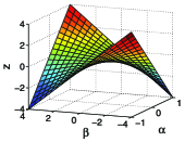
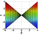
(a)	(b)
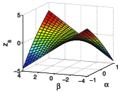
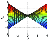
(c)	(d)

Figure 1: A geometric illustration of the smoothness of $f_{\mu}(\beta)$. (a) The 3-D plot of $z(\alpha,\beta)$, (b) the projection of (a) onto the $\beta$-$z$ space, (c) the 3-D plot of $z_{s}(\alpha,\beta)$ and (d) the projection of (c) onto the $\beta$-$z$ space.

Geometric illustration of Theorem 1. To provide insights on why $f_{\mu}({\bolds\beta})$ is a smooth function as Theorem 1 suggests, in Figure 1 we show a geometric illustration for the case of a one-dimensional parameter (i.e., $\beta\in\mathbb{R}$) with $\mu$ and $C$ set to 1. First, we show geometrically that $f_{0}(\beta)=\max_{\alpha\in[-1,1]}z(\alpha,\beta)$ with $z(\alpha,\beta)\equiv\alpha\beta$ is a nonsmooth function. The three-dimensional plot for $z(\alpha,\beta)$ with $\alpha$ restricted to $[-1,1]$ is shown in Figure 1(a). We project the surface in Figure 1(a) onto the $\beta-z$ space as shown in Figure 1(b). For each $\beta$, the value of $f_{0}(\beta)$ is the highest point along the $z$-axis since we maximize over $\alpha$ in $[-1,1]$. We can see that $f_{0}(\beta)$ is composed of two segments with a sharp point at $\beta=0$ and hence is nonsmooth. Now, we introduce $d(\alpha)=\frac{1}{2}\alpha^{2}$, let $z_{s}(\alpha,\beta)\equiv\alpha\beta-\frac{1}{2}\alpha^{2}$ and $f_{\mu}(\beta)=\max_{\alpha\in[-1,1]}z_{s}(\alpha,\beta)$. The three-dimensional plot for $z_{s}(\alpha,\beta)$ with $\alpha$ restricted to $[-1,1]$ is shown in Figure 1(c). Similarly, we project the surface in Figure 1(c) onto the $\beta-z_{s}$ space as shown in Figure 1(d). For fixed $\beta$, the value of $f_{\mu}(\beta)$ is the highest point along the $z$-axis. In Figure 1(d), we can see that the sharp point at $\beta=0$ is removed and $f_{\mu}(\beta)$ becomes smooth.

To compute the $\nabla f_{\mu}({\bolds\beta})$ and $L_{\mu}$, we need to know ${\bolds\alpha}^{\ast}$ and $\|C\|$. We present the closed-form equations for ${\bolds\alpha}^{\ast}$ and $\|C\|$ for the overlapping-group-lasso penalty and graph-guided-fused-lasso penalty in the following propositions. The proof is presented in the Appendix.

[(1)]

${\bolds\alpha}^{\ast}$ under overlapping-group-lasso penalty.

Proposition 1

Let ${\bolds\alpha}^{\ast}$, which is composed of $\{{\bolds\alpha}^{\ast}_{g}\}_{g\in\mathcal{G}}$, be the optimal solution to (10) for the overlapping-group-lasso penalty in (3). For any ${g\in\mathcal{G}}$,

$${\bolds\alpha}^{\ast}_{g}=S\biggl{(}\frac{\gamma w_{g}{\bolds\beta}_{g}}{\mu}\biggr{)},$$

where $S$ is the projection operator which projects any vector ${\mathbf{u}}$ to the $\ell_{2}$ ball:

$$S({\mathbf{u}})=\cases{\dfrac{{\mathbf{u}}}{\|{\mathbf{u}}\|_{2}},&\quad$\|{\mathbf{u}}\|_{2}>1$,\vspace*{2pt}\cr{\mathbf{u}},&\quad$\|{\mathbf{u}}\|_{2}\leq 1$.}$$

In addition, we have $\|C\|=\gamma\max_{j\in\{1,\ldots,J\}}\sqrt{\sum_{{g\in\mathcal{G}}\ \mathrm{s.t.}\ j\in g}(w_{g})^{2}}$.

${\bolds\alpha}^{\ast}$ under graph-guided-fused-lasso penalty.

Proposition 2

Let ${\bolds\alpha}^{\ast}$ be the optimal solution of (10) for the graph-guided-fused-lasso penalty in (4). Then, we have

$${\bolds\alpha}^{\ast}=S\biggl{(}\frac{C{\bolds\beta}}{\mu}\biggr{)},$$

where $S$ is the projection operator defined as follows:

$$S(x)=\cases{x,&\quad if $-1\leq x\leq 1$,\cr 1,&\quad if $x>1$,\cr-1,&\quad if $x<-1$.}$$

For any vector ${\bolds\alpha}$, $S({\bolds\alpha})$ is defined as applying $S$ on each and every entry of ${\bolds\alpha}$.

$\|C\|$ is upper-bounded by $\sqrt{2\gamma^{2}\max_{j\in V}d_{j}}$, where

$$d_{j}=\sum_{e\in E\ \mathrm{s.t.}\ e\ \mathrm{incident}\ \mathrm{on}\ j}(\tau(r_{e}))^{2}$$ (12)

for $j\in V$ in graph $G$, and this bound is tight. Note that when $\tau(r_{e})=1$ for all $e\in E$, $d_{j}$ is simply the degree of the node $j$.

3.3 Smoothing proximal gradient descent

Given the smooth approximation to the nonsmooth structured sparsity-inducing penalties, now, we apply the fast iterative shrinkage-thresholding algorithm (FISTA) [Beck and Teboulle (2009), Tseng (2008)] to solve a generically reformulated optimization problem, using the gradient information from Theorem 1. We substitute the penalty term $\Omega({\bolds\beta})$ in (2) with its smooth approximation $f_{\mu}({\bolds\beta})$ to obtain the following optimization problem:

$$\min_{{\bolds\beta}}\widetilde{f}({\bolds\beta})\equiv g({\bolds\beta})+f_{\mu}({\bolds\beta})+\lambda\|{\bolds\beta}\|_{1}.$$ (13)

Let

$$h({\bolds\beta})=g({\bolds\beta})+f_{\mu}({\bolds\beta})=\tfrac{1}{2}\|{\mathbf{y}}-{\mathbf{X}}{\bolds\beta}\|_{2}^{2}+f_{\mu}({\bolds\beta})$$ (14)

be the smooth part of $\widetilde{f}({\bolds\beta})$. According to Theorem 1, the gradient of $h({\bolds\beta})$ is given as

$$\nabla h({\bolds\beta})={\mathbf{X}}^{T}({\mathbf{X}}{\bolds\beta}-{\mathbf{y}})+C^{T}{\bolds\alpha}^{\ast}.$$ (15)

Moreover, $\nabla h({\bolds\beta})$ is Lipschitz-continuous with the Lipschitz constant,

$$L=\lambda_{\max}({\mathbf{X}}^{T}{\mathbf{X}})+L_{\mu}=\lambda_{\max}({\mathbf{X}}^{T}{\mathbf{X}})+\frac{\|C\|^{2}}{\mu},$$ (16)

where $\lambda_{\max}({\mathbf{X}}^{T}{\mathbf{X}})$ is the largest eigenvalue of $({\mathbf{X}}^{T}{\mathbf{X}})$.

Since $\widetilde{f}({\bolds\beta})$ only involves a very simple nonsmooth part (i.e., the $\ell_{1}$-norm penalty), we can adopt FISTA [Beck and Teboulle (2009), Tseng (2008)] to minimize $\widetilde{f}({\bolds\beta})$ as shown in Algorithm 1. Algorithm 1 alternates between the sequences $\{w^{t}\}$ and $\{{\bolds\beta}^{t}\}$ and $\theta_{t}$ can be viewed as a special “step-size,” which determines the relationship between $\{w^{t}\}$ and $\{{\bolds\beta}^{t}\}$ as in Step 4 of Algorithm 1. As shown in Beck and Teboulle (2009), such a way of setting $\theta_{t}$ leads to Lemma 1 in the Appendix, which further guarantees the convergence result in Theorem 2.

Algorithm 1 Smoothing proximal gradient descent (SPG) for structured sparse regression

Input: ${\mathbf{X}}$, ${\mathbf{y}}$, $C$, ${\bolds\beta}^{0}$, Lipschitz constant $L$, desired accuracy $\varepsilon$.

Initialization: set $\mu=\frac{\varepsilon}{2D}$ where $D=\max_{{\bolds\alpha}\in\mathcal{Q}}\frac{1}{2}\|{\bolds\alpha}\|_{2}^{2}$ ($D=|\mathcal{G}|/2$ for the overlapping-group-lasso penalty and $D=|E|/2$ for the graph-guided-fused-lasso penalty), $\theta_{0}=1$, ${\mathbf{w}}^{0}={\bolds\beta}^{0}$.

Iterate: For $t=0,1,2,\ldots,$ until convergence of ${\bolds\beta}^{t}$: [1.]

Compute $\nabla h({\mathbf{w}}^{t})$ according to (15).

Solve the proximal operator associated with the $\ell_{1}$-norm:

$${\bolds\beta}^{t+1} = \mathop{\arg\min}_{{\bolds\beta}}Q_{L}({\bolds\beta},{\mathbf{w}}^{t})$$

$$\equiv h({\mathbf{w}}^{t})+\langle{\bolds\beta}-{\mathbf{w}}^{t},\nabla h({\mathbf{w}}^{t})\rangle+\lambda\|{\bolds\beta}\|_{1}+\frac{L}{2}\|{\bolds\beta}-{\mathbf{w}}^{t}\|_{2}^{2}.$$

Set $\theta_{t+1}=\frac{2}{t+3}$.

Set ${\mathbf{w}}^{t+1}={\bolds\beta}^{t+1}+\frac{1-\theta_{t}}{\theta_{t}}\theta_{t+1}({\bolds\beta}^{t+1}-{\bolds\beta}^{t})$. Output: $\widehat{{\bolds\beta}}={\bolds\beta}^{t+1}$.

Rewriting $Q_{L}({\bolds\beta},{\mathbf{w}}^{t})$ in (1),

$$Q_{L}({\bolds\beta},{\mathbf{w}}^{t})=\frac{1}{2}\biggl{\|}{\bolds\beta}-\biggl{(}{\mathbf{w}}^{t}-\frac{1}{L}\nabla h({\mathbf{w}}^{t})\biggr{)}\biggr{\|}_{2}^{2}+\frac{\lambda}{L}\|{\bolds\beta}\|_{1}.$$

Letting ${\mathbf{v}}=({\mathbf{w}}^{t}-\frac{1}{L}\nabla h({\mathbf{w}}^{t}))$, the closed-form solution for ${\bolds\beta}^{t+1}$ can be obtained by soft-thresholding [Friedman et al. (2007)] as presented in the next proposition.

Proposition 3

The closed-form solution of

$$\min_{{\bolds\beta}}\frac{1}{2}\|{\bolds\beta}-{\mathbf{v}}\|_{2}^{2}+\frac{\lambda}{L}\|{\bolds\beta}\|_{1}$$

can be obtained by the soft-thresholding operation:

$$\beta_{j}=\operatorname{sign}(v_{j})\max\biggl{(}0,|v_{j}|-\frac{\lambda}{L}\biggr{)},\qquad j=1,\ldots,J.$$ (18)

An important advantage of using the proximal operator associated with the $\ell_{1}$-norm $Q_{L}({\bolds\beta},{\mathbf{w}}^{t})$ is that it can provide us with sparse solutions, where the coefficients for irrelevant inputs are set exactly to zeros, due to the soft-thresholding operation in (18). When the term $\lambda\|{\bolds\beta}\|_{1}$ is not included in the objective, for overlapping group lasso, we can only obtain the group level sparsity but not the individual feature level sparsity inside each group. However, as for optimization, Algorithm 1 still applies in the same way. The only difference is that Step 2 of Algorithm 1 becomes ${\bolds\beta}^{t+1}=\mathop{\arg\min}_{{\bolds\beta}}h({\mathbf{w}}^{t})+\langle{\bolds\beta}-{\mathbf{w}}^{t},\nabla h({\mathbf{w}}^{t})\rangle+\frac{L}{2}\|{\bolds\beta}-{\mathbf{w}}^{t}\|_{2}^{2}={\mathbf{w}}^{t}-\frac{1}{L}\nabla h({\mathbf{w}}^{t})$. Since there is no soft-thresholding step, the obtained solution $\widehat{{\bolds\beta}}$ has no exact zeros. We then need to set a threshold (e.g., $10^{-5}$) and select the relevant groups which contain the variables with the parameter above this threshold.

3.4 Issues on the computation of the Lipschitz constant

When $J$ is large, the computation of $\lambda_{\max}({\mathbf{X}}^{T}{\mathbf{X}})$ and hence the Lipschitz constant $L$ could be very expensive. To further accelerate Algorithm 1, a line search backtracking step could be used to dynamically assign a constant $L_{t}$ for the proximal operator in each iteration [Beck and Teboulle (2009)]. More specifically, given any positive constant $R$, let

$$Q_{R}({\bolds\beta},{\mathbf{w}}^{t})=h({\mathbf{w}}^{t})+\langle{\bolds\beta}-{\mathbf{w}}^{t},\nabla h({\mathbf{w}}^{t})\rangle+\lambda\|{\bolds\beta}\|_{1}+\frac{R}{2}\|{\bolds\beta}-{\mathbf{w}}^{t}\|_{2}^{2}$$

and

$${\bolds\beta}^{t+1}\equiv{\bolds\beta}_{R}({\mathbf{w}}^{t})=\mathop{\arg\min}_{{\bolds\beta}}Q_{R}({\bolds\beta},{\mathbf{w}}^{t}).$$

The key to guarantee the convergence rate of Algorithm 1 is to ensure that the following inequality holds for each iteration:

$$\widetilde{f}({\bolds\beta}^{t+1})=h({\bolds\beta}^{t+1})+\lambda\|{\bolds\beta}^{t+1}\|_{1}\leq Q_{R}({\bolds\beta}^{t+1},{\mathbf{w}}^{t}).$$ (19)

It is easy to check that when $R$ is equal to the Lipschitz constant $L$, it will satisfy the above inequality for any ${\bolds\beta}^{t+1}$ and ${\mathbf{w}}^{t}$. However, when it is difficult to compute the Lipschitz constant, instead of using a global constant $L$, we could find a sequence $\{L_{t}\}_{t=0}^{T}$ such that $L_{t+1}$ satisfies the inequality (19) for the $t$th iteration. In particular, we start with any small constant $L_{0}$. For each iteration, we find the smallest integer $a\in\{0,1,2,\ldots\}$ such that by setting $L_{t+1}=\tau^{a}L_{t}$, where $\tau>1$ is a predefined scaling factor, we have

$$\widetilde{f}({\bolds\beta}_{L_{t+1}}({\mathbf{w}}^{t}))\leq Q_{L_{t+1}}({\bolds\beta}_{L_{t+1}}({\mathbf{w}}^{t}),{\mathbf{w}}^{t}).$$ (20)

Then we set ${\bolds\beta}^{t+1}={\bolds\beta}_{L_{t+1}}({\mathbf{w}}^{t})\equiv\mathop{\arg\min}Q_{L_{t+1}}({\bolds\beta},{\mathbf{w}}^{t})$.

3.5 Convergence rate and time complexity

Although we optimize the approximation function $\widetilde{f}({\bolds\beta})$ rather than the original $f({\bolds\beta})$ directly, it can be proven that $f(\widehat{{\bolds\beta}})$ is sufficiently close to the optimal objective value of the original function $f({\bolds\beta}^{*})$. The convergence rate of Algorithm 1 is presented in the next theorem.

Theorem 2.

Let ${\bolds\beta}^{\ast}$ be the optimal solution to (2) and ${\bolds\beta}^{t}$ be the approximate solution at the $t$th iteration in Algorithm 1. If we require $f({\bolds\beta}^{t})-f({\bolds\beta}^{\ast})\leq\varepsilon$ where $f$ is the original objective, and set $\mu=\frac{\varepsilon}{2D}$, then the number of iterations $t$ is upper-bounded by

$$\sqrt{\frac{4\|{\bolds\beta}^{\ast}-{\bolds\beta}^{0}\|_{2}^{2}}{\varepsilon}{\biggl{(}\lambda_{\max}({\mathbf{X}}^{T}{\mathbf{X}})+\frac{2D\|C\|^{2}}{\varepsilon}\biggr{)}}}.$$ (21)

The key idea behind the proof of this theorem is to decompose $f({\bolds\beta}^{t})-f({\bolds\beta}^{\ast})$ into three parts: (i) $f({\bolds\beta}^{t})-\widetilde{f}({\bolds\beta}^{t})$, (ii) $\widetilde{f}({\bolds\beta}^{t})-\widetilde{f}({\bolds\beta}^{\ast})$ and (iii) $\widetilde{f}({\bolds\beta}^{\ast})-f({\bolds\beta}^{\ast})$. (i) and (iii) can be bounded by the gap of the approximation $\mu D$; and (ii) only involves the function $\widetilde{f}$ and can be upper bounded by $O(\frac{1}{t^{2}})$ as shown in Beck and Teboulle (2009). We obtain (21) by balancing these three terms. The details of the proof are presented in the Appendix. According to Theorem 2, Algorithm 1 converges in $O(\frac{\sqrt{2D}}{\varepsilon})$ iterations, which is much faster than the subgradient method with the convergence rate of $O(\frac{1}{\varepsilon^{2}})$. Note that the convergence rate depends on $D$ through the term $\sqrt{2D}$, and the $D$ depends on the problem size.

Remark 2.

Since there is no line search in Algorithm 1, we cannot guarantee that the objective values are monotonically decreasing over iterations theoretically. But empirically, based on our own experience, the objective values always decrease over iterations. One simple strategy to guarantee the monotone decreasing property is to first compute $\widetilde{{\bolds\beta}}{}^{t+1}=\mathop{\arg\min}_{{\bolds\beta}}Q_{L}({\bolds\beta},{\mathbf{w}}^{t})$ and then set ${\bolds\beta}^{t+1}=\mathop{\arg\min}_{{\bolds\beta}\in\{\widetilde{{\bolds\beta}}{}^{t+1},{\bolds\beta}^{t}\}}f({\bolds\beta})$.

Remark 3.

Theorem 2 only shows the convergence rate for the objective value. As for the estimator ${\bolds\beta}^{t}$, since it is a convex optimization problem, it is well known that ${\bolds\beta}^{t}$ will eventually converge to ${\bolds\beta}^{*}$. However, the speed of convergence of ${\bolds\beta}^{t}$ to ${\bolds\beta}^{*}$ depends on the structure of the input ${\mathbf{X}}$. If $h({\bolds\beta})$ is a strongly convex function with the strong convexity parameter, $\sigma>0$. In our problem, it is equivalent to saying that ${\mathbf{X}}^{T}{\mathbf{X}}$ is a nonsingular matrix with the smallest eigenvalue $\sigma>0$. Then we can show that if $f({\bolds\beta}^{t})-f({\bolds\beta}^{*})\leq\varepsilon$ at the convergence, then $\|{\bolds\beta}^{t}-{\bolds\beta}^{*}\|_{2}\leq\sqrt{\frac{2\varepsilon}{\sigma}}$. In other words, ${\bolds\beta}^{t}$ converges to ${\bolds\beta}^{*}$ in $\ell_{2}$-distance at the rate of $O(\frac{1}{\varepsilon^{2}})$. For general high-dimensional sparse learning problems with $J>N$, ${\mathbf{X}}^{T}{\mathbf{X}}$ is singular and, hence, the optimal solution ${\bolds\beta}^{*}$ is not unique. In such a case, one can only show that ${\bolds\beta}^{t}$ will converge to one of the optimal solutions. But the speed of the convergence of $\|{\bolds\beta}^{t}-{\bolds\beta}^{*}\|_{2}$ or its relationship with $f({\bolds\beta}^{t})-f({\bolds\beta}^{*})$ is widely recognized as an open problem in the optimization community.

As for the time complexity, the main computational cost in each iteration comes from calculating the gradient $\nabla h({\mathbf{w}}_{t})$. Therefore, SPG shares almost the same per-iteration time as the subgradient descent but with a faster convergence rate. In more details, if $J<N$ and ${\mathbf{X}}^{T}{\mathbf{X}}$ and ${\mathbf{X}}^{T}{\mathbf{y}}$ can be pre-computed and stored in memory, the computation of the first part of $\nabla h({\mathbf{w}}_{t})$, $({\mathbf{X}}^{T}{\mathbf{X}}){\mathbf{w}}_{t}-({\mathbf{X}}^{T}{\mathbf{y}})$, takes the time complexity of $O(J^{2})$. Otherwise, if $J>N$, we can compute this part by ${\mathbf{X}}^{T}({\mathbf{X}}{\mathbf{w}}_{t}-{\mathbf{y}})$, which takes the time complexity of $O(JN)$. As for the generic solver, IPM for SOCP for overlapping group lasso or IPM for QP for graph-guided fused lasso, although it converges in fewer iterations [i.e., $\log(\frac{1}{\varepsilon})$], its per-iteration complexity is higher by orders of magnitude than ours as shown in Table 1. In addition to time complexity, IPM requires the pre-storage of ${\mathbf{X}}^{T}{\mathbf{X}}$ and each IPM iteration requires significantly more memory to store the Newton linear system. Therefore, the SPG is much more efficient and scalable for large-scale problems.

Table 1: Comparison of per-iteration time complexity

	Overlapping group lasso	Graph-guided fused lasso
SPG	$O(J\min(J,N)+\sum_{{g\in\mathcal{G}}}|g|)$	$O(J\min(J,N)+|E|)$
IPM	$O((J+|\mathcal{G}|)^{2}(N+\sum_{{g\in\mathcal{G}}}|g|))$	$O((J+|E|)^{3})$

3.6 Summary and discussions

The insight of our work was drawn from two lines of earlier works. The first one is the proximal gradient methods (e.g., Nesterov’s composite gradient method [Nesterov (2007)], FISTA [Beck and Teboulle (2009)]. They have been widely adopted to solve optimization problems with a convex loss and a relatively simple nonsmooth penalty, achieving $O(\frac{1}{\sqrt{\varepsilon}})$ convergence rate. However, the complex structure of the nonseparable penalties considered in this paper makes it intractable to solve the proximal operator exactly. This is the challenge that we circumvent via smoothing.

The general idea of the smoothing technique used in this paper was first introduced by Nesterov (2005). The algorithm presented in Nesterov (2005) only works for smooth problems so that it has to smooth out the entire nonsmooth penalty. Our approach separates the simple nonsmooth $\ell_{1}$-norm penalty from the complex structured sparsity-inducing penalties. In particular, when an $\ell_{1}$-norm penalty is used to enforce the individual-feature-level sparsity (which is especially necessary for fused lasso), we smooth out the complex structured-sparsity-inducing penalty while leaving the simple $\ell_{1}$-norm as it is. One benefit of our approach is that it can lead to solutions with exact zeros for irrelevant features due to the $\ell_{1}$-norm penalty and hence avoid the post-processing (i.e., truncation) step. Moreover, the algorithm in Nesterov (2005) requires the condition that ${\bolds\beta}$ is bounded and that the number of iterations is predefined, which are impractical for real applications.

As for the convergence rate, the gap between $O(\frac{1}{\varepsilon})$ and the optimal rate $O(\frac{1}{\sqrt{\varepsilon}})$ is due to the approximation of the structured sparsity-inducing penalty. It is possible to show that if ${\mathbf{X}}$ has a full column rank, $O(\frac{1}{\sqrt{\varepsilon}})$ can be achieved by a variant of the excessive gap method [Nesterov (2003)]. However, such a rate cannot be easily obtained for sparse regression problems where $J>N$. For some special cases as discussed in the next section, such as tree-structured or the $\ell_{1}/\ell_{\infty}$ mixed-norm based overlapping groups, $O(\frac{1}{\sqrt{\varepsilon}})$ can be achieved at the expense of more computation time for solving the proximal operator. It remains an open question whether we can further boost the generally-applicable SPG method to achieve $O(\frac{1}{\sqrt{\varepsilon}})$.

4 Related optimization methods

4.1 Connections with majorization–minimization

The idea of constructing a smoothing approximation has also been adopted in another widely used optimization method, majorization–minimization (MM) for minimization problem (or minorization–maximization for maximization problem) [Lange (2004)]. To minimize a given objective, MM replaces the difficult-to-optimize objective function with a simple (and smooth in most cases) surrogate function which majorizes the objective. It minimizes the surrogate function and iterates such a procedure. The difference between our approach and MM is that our approximation is a uniformly smooth lower bound of the objective with a bounded gap, whereas the surrogate function in MM is an upper bound of the objective. In addition, MM is an iterative procedure which iteratively constructs and minimizes the surrogate function, while our approach constructs the smooth approximation once and then applies the proximal gradient descent to optimize it. With the quadratic surrogate functions for the $\ell_{2}$-norm and fused-lasso penalty derived in Wu and Lange (2008) and Zhang et al. (2010), one can easily apply MM to solve the structured sparse regression problems. However, in our problems, the Hessian matrix in the quadratic surrogate will no longer have a simple structure (e.g., tridiagonal symmetric structure in chain-structured fused signal approximator). Therefore, one may need to apply the general optimization methods, for example, conjugate-gradient or quasi-Newton method, to solve a series of quadratic surrogate functions. In addition, since the objective functions considered in our paper are neither smooth nor strictly convex, the local and global convergence results for MM in Lange (2004) cannot be applied. It seems to us still an open problem to derive the local, global convergence and the convergence rate for MM for the general nonsmooth convex optimization.

Recently, many first-order approaches have been developed for various subclasses of overlapping group lasso and graph-guided fused lasso. Below, we provide a survey of these methods:

4.2 Related work for mixed-norm based group-lasso penalty

Most of the existing optimization methods developed for mixed-norm penalties can handle only a specific subclass of the general overlapping-group-lasso penalties. Most of these methods use the proximal gradient framework [Beck and Teboulle (2009), Nesterov (2007)] and focus on the issue of how to exactly solve the proximal operator. For nonoverlapping groups with the $\ell_{1}/\ell_{2}$ or $\ell_{1}/\ell_{\infty}$ mixed-norms, the proximal operator can be solved via a simple projection [Duchi and Singer (2009), Liu, Ji and Ye (2009)]. A one-pass coordinate ascent method has been developed for tree-structured groups with the $\ell_{1}/\ell_{2}$ or $\ell_{1}/\ell_{\infty}$ [Liu and Ye (2010b), Jenatton et al. (2010)], and quadratic min-cost network flow for arbitrary overlapping groups with the $\ell_{1}/\ell_{\infty}$ [Mairal et al. (2010)].

= No overlap No overlap Overlap Overlap Overlap Overlap Method $\bolds{\ell_{1}/\ell_{2}}$ $\bolds{\ell_{1}/\ell_{\infty}}$ tree $\bolds{\ell_{1}/\ell_{2}}$ tree $\bolds{\ell_{1}/\ell_{\infty}}$ arbitrary $\bolds{\ell_{1}/\ell_{2}}$ arbitrary $\bolds{\ell_{1}/\ell_{\infty}}$ Projection $O(\frac{1}{\sqrt{\varepsilon}})$, $O(J)$ $O(\frac{1}{\sqrt{\varepsilon}})$, $O(J\log J)$ N.A. N.A. N.A. N.A.    [Liu, Ji and Ye (2009)] Coordinate ascent $O(\frac{1}{\sqrt{\varepsilon}})$, $O(J)$ $O(\frac{1}{\sqrt{\varepsilon}})$, $O(J\log J)$ $O(\frac{1}{\sqrt{\varepsilon}})$, $O(\frac{1}{\sqrt{\varepsilon}})$, N.A. N.A.    [Jenatton et al. (2010), $O({\sum_{g\in\mathcal{G}}}|g|)$ $O({\sum_{g\in\mathcal{G}}}{|g|\log}|g|)$    Liu and Ye (2010b)] Network Flow [Mairal N.A. $O(\frac{1}{\sqrt{\varepsilon}})$, quadratic N.A. $O(\frac{1}{\sqrt{\varepsilon}})$, quadratic N.A. $O(\frac{1}{\sqrt{\varepsilon}})$, quadratic    et al. (2010)] min-cost flow min-cost flow min-cost flow FOBOS [Duchi and $O(\frac{1}{\varepsilon})$, $O(J)$ $O(\frac{1}{\varepsilon})$, $O(J\log J)$ $O(\frac{1}{\varepsilon})$, $O(\frac{1}{\varepsilon})$, $O(\frac{1}{\varepsilon^{2}})$, $O(\frac{1}{\varepsilon})$, quadratic    Singer (2009)] $O({\sum_{g\in\mathcal{G}}}|g|)$ $O({\sum_{g\in\mathcal{G}}}{|g|\log}|g|)$ $O({\sum_{g\in\mathcal{G}}}|g|)$ min-cost flow (subgradient) SPG $O(\frac{1}{\varepsilon})$, $O(J)$ $O(\frac{1}{\varepsilon})$, $O(J\log J)$ $O(\frac{1}{\varepsilon})$, $O(\frac{1}{\varepsilon})$, $O(\frac{1}{\varepsilon})$, $O(\frac{1}{\varepsilon})$, $O({\sum_{g\in\mathcal{G}}}|g|)$ $O({\sum_{g\in\mathcal{G}}}{|g|\log}|g|)$ $O({\sum_{g\in\mathcal{G}}}|g|)$ $O({\sum_{g\in\mathcal{G}}}{|g|\log}|g|)$

Table 2: Comparisons of different first-order methods for optimizing mixed-norm based overlapping-group-lasso penalties

Table 2 summarizes the applicability, the convergence rate and the per-iteration time complexity for the available first-order methods for different subclasses of group lasso penalties. More specifically, the methods in the first three rows adopt the proximal gradient framework. The first column of these rows gives the solver for the proximal operator. Each entry in Table 2 contains the convergence rate and the per-iteration time complexity. For the sake of simplicity, for all methods, we omit the time for computing the gradient of the loss function which is required for all of the methods [i.e., $\nabla g({\bolds\beta})$ with $O(J^{2})$]. The per-iteration time complexity in the table may come from the computation of the proximal operator or subgradient of the penalty. “N.A.” stands for “not applicable” or no guarantee in the convergence. As we can see from Table 2, although our method is not the most ideal one for some of the special cases, our method along with FOBOS [Duchi and Singer (2009)] are the only generic first-order methods that can be applied to all subclasses of the penalties.

As we can see from Table 2, for arbitrary overlaps with the $\ell_{1}/\ell_{\infty}$, although the method proposed in Mairal et al. (2010) achieves $O(\frac{1}{\sqrt{\varepsilon}})$ convergence rate, the per-iteration complexity can be high due to solving a quadratic min-cost network flow problem. From the worst-case analysis, the per-iteration time complexity for solving the network flow problem in Mairal et al. (2010) is at least $O(|V||E|)=O((J+|\mathcal{G}|)(|\mathcal{G}|+J+\sum_{g\in\mathcal{G}}|g|))$, which is much higher than our method with $O(\sum_{g\in\mathcal{G}}{|g|\log}|g|)$. More importantly, for the case of arbitrary overlaps with the $\ell_{1}/\ell_{2}$, our method has a superior convergence rate to all the other methods.

In addition to these methods, an active-set algorithm was proposed that can be applied to the square of the $\ell_{1}/\ell_{2}$ mixed-norm with overlapping groups [Jenatton, Audibert and Bach (2009)]. This method formulates each subproblem involving only the active variables either as an SOCP, which can be computationally expensive for a large active set, or as a jointly convex problem with auxiliary variables, which is then solved by an alternating gradient descent. The latter approach involves an expensive matrix inversion at each iteration and lacks the global convergence rate. Another method [Liu and Ye (2010a)] was proposed for the overlapping group lasso which approximately solves the proximal operator. However, the convergence of this type of approach cannot be guaranteed, since the error introduced in each proximal operator will be accumulated over iterations.

4.3 Related work for fused lasso

For the graph-guided-fused-lasso penalty, when the structure is a simple chain, the pathwise coordinate descent method [Friedman et al. (2007)] can be applied. For the general graph structure, a first-order method that approximately solves the proximal operator was proposed in Liu, Yuan and Ye (2010). However, the convergence cannot be guaranteed due to the errors introduced in computing the proximal operator over iterations.

Recently, two different path algorithms have been proposed [Tibshirani and Taylor (2010), Zhou and Lange (2011)] that can be used to solve the graph-guided fused lasso as a special case. Unlike the traditional optimization methods that solve the problem for a fixed regularization parameter, they solve the entire path of solutions, and, thus, have great practical advantages. In addition, for both methods, updating solutions from one hitting time to another is computationally very cheap. More specifically, a QR decomposition based updating scheme was proposed in Tibshirani and Taylor (2010) and the updating in Zhou and Lange (2011) can be done by an efficient sweep operation.

However, for high-dimensional data with $J\gg N$, the path algorithms can have the following problems: [(1)]

For a general design matrix ${\mathbf{X}}$ other than the identity matrix, the method in Tibshirani and Taylor (2010) needs to first compute the pseudo-inverse of ${\mathbf{X}}\dvtx{\mathbf{X}}^{+}=({\mathbf{X}}^{T}{\mathbf{X}})^{+}{\mathbf{X}}^{T}$, which could be computationally expensive for large $J$.

The original version of the algorithms in Tibshirani and Taylor (2010) and Zhou and Lange (2011) requires that ${\mathbf{X}}$ has a full column rank. When $J>N$, although one can add an extra $\varepsilon\|{\bolds\beta}\|_{2}^{2}$ term, this changes the original objective value especially when $\varepsilon$ is large. For smaller $\varepsilon$, the matrix $({\mathbf{X}}^{*})^{T}{\mathbf{X}}^{*}$ with ${\mathbf{X}}^{*}=\bigl{[}{{\mathbf{X}}\atop\varepsilon I}\bigr{]}$ is highly ill-conditioned; and hence computing its inverse as the initialization step in Tibshirani and Taylor (2010) is very difficult. There is no known result on how to balance this trade-off.

In both Tibshirani and Taylor (2010) and Zhou and Lange (2011), the authors extend their algorithm to deal with the case when ${\mathbf{X}}$ does not have a full column rank. The extended version requires a Gramm–Schmidt process as the initialization, which could take some extra time.

In Table 3 we present the comparisons for different methods. From our analysis, the method in Zhou and Lange (2011) is more efficient than the one in Tibshirani and Taylor (2010) since it avoids the heavy computation of the pseudo-inverse of ${\mathbf{X}}$. In practice, if ${\mathbf{X}}$ has a full column rank and one is interested in solutions on the entire path, the method in Zhou and Lange (2011) is very efficient and faster than our method. Instead, when $J\gg N$, the path following methods may require a time-consuming preprocessing procedure.

Table 3: Comparisons of different methods for optimizing graph-guided fused lasso

Method	Preprocessing	Per-iteration	No. of
and condition	time	time complexity	iterations
[Zhou and	$O(J^{3})$	$O((|E|+J)^{2})$	$O(|E|+J)$
Lange (2011)]
(${\mathbf{X}}$ full column
rank, entire path)
[Tibshirani and	$O(J^{3}+N(|E|+J)\quad\hskip 4.0pt$	$O(\min((|E|+J)^{2},N^{2}))$	$O(|E|+J)$
Taylor (2010)]	$\quad\hskip 4.0pt\times\min((|E|+J),N))$		(lower bound)
(${\mathbf{X}}$ full column
rank, entire path)
[Tibshirani and	$O(J^{3}+J^{2}N+(|E|+J)^{2}N)$	$O(N^{2})$	$O(|E|+J)$
Taylor (2010)]			(lower bound)
(${\mathbf{X}}$ not full column
rank, entire path)
SPG (single	$O(NJ^{2})$	$O(J^{2}+|E|)$	$O(\frac{1}{\varepsilon})$
regularization
parameter)

5 Extensions to multi-task regression with structures on outputs

The structured sparsity-inducing penalties as discussed in the previous section can be similarly used in the multi-task regression setting [Kim and Xing (2010), Kim, Sohn and Xing (2009)], where the prior structural information is available for the outputs instead of inputs. For example, in genetic association analysis, where the goal is to discover few genetic variants or single nucleotide polymorphisms (SNPs) out of millions of SNPs (inputs) that influence phenotypes (outputs) such as gene expression measurements, the correlation structure of the phenotypes can be naturally represented as a graph, which can be used to guide the selection of SNPs as shown in Figure 2. Then, the graph-guided-fused-lasso penalty can be used to identify SNPs that are relevant jointly to multiple related phenotypes.

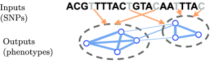
Figure 2: Illustration of the multi-task regression with graph structure on outputs.

In a sparse multi-task regression with structure on the output side, we encounter the same difficulties of optimizing with nonsmooth and nonseparable penalties as in the previous section, and the SPG can be extended to this problem in a straightforward manner. Due to the importance of this class of problems and its applications, in this section, we briefly discuss how our method can be applied to the multi-task regression with structured-sparsity-inducing penalties.

5.1 Multi-task linear regression regularized by structured sparsity-inducing penalties

For the simplicity of illustration, we assume all different tasks share the same input matrix. Let ${\mathbf{X}}\in\mathbb{R}^{N\times J}$ denote the matrix of input data for $J$ inputs and ${\mathbf{Y}}\in\mathbb{R}^{N\times K}$ denote the matrix of output data for $K$ outputs over $N$ samples. We assume a linear regression model for each of the $k$th outputs: ${\mathbf{y}}_{k}={\mathbf{X}}{\bolds\beta}_{k}+{\bolds\varepsilon}_{k},\forall k=1,\ldots,K$, where ${\bolds\beta}_{k}=[\beta_{1k},\ldots,\beta_{Jk}]^{T}$ is the regression coefficient vector for the $k$th output and ${\bolds\varepsilon}_{k}$ is Gaussian noise. Let ${\mathbf{B}}=[{\bolds\beta}_{1},\ldots,{\bolds\beta}_{K}]\in\mathbb{R}^{J\times K}$ be the matrix of regression coefficients for all of the $K$ outputs. Then, the multi-task (or multivariate-response) structured sparse regression problem can be naturally formulated as the following optimization problem:

$$\min_{{\mathbf{B}}\in\mathbb{R}^{J\times K}}f({\mathbf{B}})\equiv\frac{1}{2}\|{\mathbf{Y}}-{\mathbf{X}}{\mathbf{B}}\|_{F}^{2}+\Omega({\mathbf{B}})+\lambda\|{\mathbf{B}}\|_{1},$$ (22)

where $\|\cdot\|_{F}$ denotes the matrix Frobenius norm, $\|\cdot\|_{1}$ denotes the matrix entry-wise $\ell_{1}$ norm, and $\Omega({\mathbf{B}})$ is a structured sparsity-inducing penalty with a structure over the outputs. [(1)]

Overlapping-group-lasso penalty in multi-task regression. We define the overlapping-group-lasso penalty for a structured multi-task regression as follows:

$$\Omega({\mathbf{B}})\equiv\gamma\sum_{j=1}^{J}\sum_{g\in\mathcal{G}}w_{g}\|{\bolds\beta}_{jg}\|_{2},$$ (23)

where $\mathcal{G}=\{g_{1},\ldots,g_{|\mathcal{G}|}\}$ is a subset of the power set of $\{1,\ldots,K\}$ and ${\bolds\beta}_{jg}$ is the vector of regression coefficients corresponding to outputs in group $g\dvtx\{\beta_{jk},k\in g,g\in\mathcal{G}\}$. Both the $\ell_{1}/\ell_{2}$ mixed-norm penalty for multi-task regression in Obozinski, Taskar and Jordan (2009) and the tree-structured overlapping-group-lasso penalty in Kim and Xing (2010) are special cases of (23).

Graph-guided-fused-lasso penalty in multi-task regression. Assuming that a graph structure over the $K$ outputs is given as $G$ with a set of nodes $V=\{1,\ldots,K\}$, each corresponding to an output variable and a set of edges $E$, the graph-guided-fused-lasso penalty for a structured multi-task regression is given as

$$\Omega({\mathbf{B}})=\gamma\sum_{e=(m,l)\in E}\tau(r_{ml})\sum_{j=1}^{J}|{\bolds\beta}_{jm}-\operatorname{sign}(r_{ml}){\bolds\beta}_{jl}|.$$ (24)

5.2 Smoothing proximal gradient descent

Using similar techniques in Section 3.1, $\Omega({\mathbf{B}})$ can be reformulated as

$$\Omega({\mathbf{B}})=\max_{{\mathbf{A}}\in\mathcal{Q}}\langle C{\mathbf{B}}^{T},{\mathbf{A}}\rangle,$$ (25)

where $\langle\mathbf{U},\mathbf{V}\rangle\equiv\operatorname{Tr}(\mathbf{U}^{T}\mathbf{V})$ denotes a matrix inner product. $C$ is constructed in a similar way as in (7) or (8), just by replacing the index of the input variables with the output variables, and ${\mathbf{A}}$ is the matrix of the auxiliary variables.

Then we introduce the smooth approximation of (25):

$$f_{\mu}({\mathbf{B}})=\max_{{\mathbf{A}}\in\mathcal{Q}}(\langle C{\mathbf{B}}^{T},{\mathbf{A}}\rangle-\mu\,d({\mathbf{A}})),$$ (26)

where $d({\mathbf{A}})\equiv\frac{1}{2}\|{\mathbf{A}}\|_{F}^{2}$. Following a proof strategy similar to that in Theorem 1, we can show that $f_{\mu}({\mathbf{B}})$ is convex and smooth with gradient $\nabla f_{\mu}({\mathbf{B}})=({\mathbf{A}}^{\ast})^{T}C$, where ${\mathbf{A}}^{\ast}$ is the optimal solution to (26). The closed-form solution of ${\mathbf{A}}^{\ast}$ and the Lipschitz constant for $\nabla f_{\mu}({\mathbf{B}})$ can be derived in the same way.

Table 4: Comparison of per-iteration time complexity for multi-task regression

	Overlapping group lasso	Graph-guided fused lasso
SPG	$O(JK\min(J,N)+J\sum_{{g\in\mathcal{G}}}|g|)$	$O(JK\min(J,N)+J|E|)$
IPM	$O(J^{2}(K+|\mathcal{G}|)^{2}(KN+J(\sum_{g\in\mathcal{G}}|g|)))$	$O(J^{3}(K+|E|)^{3})$

By substituting $\Omega({\mathbf{B}})$ in (22) with $f_{\mu}({\mathbf{B}})$, we can adopt Algorithm 1 to solve (22) with convergence rate of $O(\frac{1}{\varepsilon})$. The per-iteration time complexity of SPG as compared to IPM for SOCP or QP formulation is presented in Table 4. As we can see, the per-iteration complexity for SPG is linear in $\max(|K|,\sum_{g\in\mathcal{G}}|g|)$ or $\max(|K|,|E|)$, while traditional approaches based on IPM scape at least cubically to the size of outputs $K$.

6 Experiment

In this section we evaluate the scalability and efficiency of the smoothing proximal gradient method (SPG) on a number of structured sparse regression problems via simulation, and apply SPG to an overlapping group lasso problem on real genetic data.

On an overlapping group lasso problem, we compare the SPG with FOBOS [Duchi and Singer (2009)] and IPM for SOCP. On a multi-task graph-guided fused lasso problem, we compare the running time of SPG with that of the FOBOS [Duchi and Singer (2009)] and IPM for QP. Note that for FOBOS, since the proximal operator associated with $\Omega({\bolds\beta})$ cannot be solved exactly, we set the “loss function” to $l({\bolds\beta})=g({\bolds\beta})+\Omega({\bolds\beta})$ and the penalty to $\lambda\|{\bolds\beta}\|_{1}$. According to Duchi and Singer (2009), for the nonsmooth loss $l({\bolds\beta})$, FOBOS achieves $O(\frac{1}{\varepsilon^{2}})$ convergence rate, which is slower than our method.

All experiments are performed on a standard PC with 4GB RAM and the software is written in MATLAB. The main difficulty in comparisons is a fair stopping criterion. Unlike IPM, SPG and FOBOS do not generate a dual solution and, therefore, it is not possible to compute a primal-dual gap, which is the traditional stopping criterion for IPM. Here, we adopt a widely used approach for comparing different methods in the optimization literature. Since it is well known that IPM usually gives a more accurate (i.e., lower) objective, we set the objective obtained from IPM as the optimal objective value and stop the first-order methods when the objective is below 1.001 times the optimal objective. For large data sets for which IPM cannot be applied, we stop the first-order methods when the relative change in the objective is below $10^{-6}$. In addition, maximum iterations are set to 20,000.

Since our main focus is on the optimization algorithm, for the purpose of simplicity, we assume that each group in the overlapping group lasso problem receives the same amount of regularization and, hence, set the weights $w_{g}$ for all groups to be 1. In principle, more sophisticated prior knowledge of the importance for each group can be naturally incorporated into $w_{g}$. In addition, we notice that each variable $j$ with the regularization $\lambda|\beta_{j}|$ in $\lambda\|{\bolds\beta}\|_{1}$ can be viewed as a singleton group. To ease the tuning of parameters, we again assume that each group (including the singleton group) receives the same amount of regularization and, hence, constrain the regularization parameters $\lambda=\gamma$.

The smoothing parameter $\mu$ is set to $\frac{\varepsilon}{2D}$ according to Theorem 2, where $D$ is determined by the problem size. It is natural that for large-scale problems with large $D$, a larger $\varepsilon$ can be adopted without affecting the recovery quality significantly. Therefore, instead of setting $\varepsilon$, we directly set $\mu=10^{-4}$, which provided us with reasonably good approximation accuracies for different scales of problems based on our experience for a range of $\mu$ in simulations. As for FOBOS, we set the stepsize rate to $\frac{c}{\sqrt{t}}$ as suggested in Duchi and Singer (2009), where $c$ is carefully tuned to be $\frac{0.1}{\sqrt{NJ}}$ for univariate regression and $\frac{0.1}{\sqrt{NJK}}$ for multi-task regression.

6.1 Simulation study I: Overlapping group lasso

We simulate data for a univariate linear regression model with the overlapping group structure on the inputs as described below. Assuming that the inputs are ordered, we define a sequence of groups of 100 adjacent inputs with an overlap of 10 variables between two successive groups so that

$$\mathcal{G}=\bigl{\{}\{1,\ldots,100\},\{91,\ldots,190\},\ldots,\{J-99,\ldots,J\}\bigr{\}}$$

with $J=90|\mathcal{G}|+10$. We set $\beta_{j}=(-1)^{j}\exp(-(j-1)/100)$ for $1\leq j\leq J$. We sample each element of ${\mathbf{X}}$ from i.i.d. Gaussian distribution, and generate the output data from ${\mathbf{y}}={\mathbf{X}}{\bolds\beta}+{\bolds\varepsilon}$, where ${\bolds\varepsilon}\sim N(0,I_{N\times N})$.

Table 5: Comparisons of different optimization methods on the overlapping group lasso

		$\bolds{N=1}$,000		$\bolds{N=5}$,000		$\bolds{N=10}$,000
		CPU (s)	Obj.	CPU (s)	Obj.	CPU (s)	Obj.
$|\mathcal{G}|=10$ ($J=910$)
$\gamma=2$	SOCP	$103.71$	$266.683$	$493.08$	$917.132$	$3\mbox{,}777.46$	$1\mbox{,}765.518$
	FOBOS	$27.12$	$266.948$	$1.71$	$918.019$	$1.48$	$1\mbox{,}765.613$
	SPG	$0.87$	$266.947$	$0.71$	$917.463$	$1.28$	$1\mbox{,}765.692$
$\gamma=0.5$	SOCP	$106.02$	$83.304$	$510.56$	$745.102$	$3\mbox{,}585.77$	$1\mbox{,}596.418$
	FOBOS	$32.44$	$82.992$	$4.98$	$745.788$	$4.65$	$1\mbox{,}597.531$
	SPG	$0.42$	$83.386$	$0.41$	$745.104$	$0.69$	$1\mbox{,}596.452$
$|\mathcal{G}|=50$ ($J=4\mbox{,}510$)
$\gamma=10$	SOCP	$4\mbox{,}144.20$	$1\mbox{,}089.014$	–	–	–	–
	FOBOS	$476.91$	$1\mbox{,}191.047$	$394.75$	$1\mbox{,}533.314$	$79.82$	$2\mbox{,}263.494$
	SPG	$56.35$	$1\mbox{,}089.052$	$77.61$	$1\mbox{,}533.318$	$78.90$	$2\mbox{,}263.601$
$\gamma=2.5$	SOCP	$3\mbox{,}746.43$	$277.911$	–	–	–	–
	FOBOS	$478.62$	$286.327$	$867.94$	$559.251$	$183.72$	$1\mbox{,}266.728$
	SPG	$33.09$	$277.942$	$30.13$	$504.337$	$26.74$	$1\mbox{,}266.723$
$|\mathcal{G}|=100$ ($J=9\mbox{,}010$)
$\gamma=20$	FOBOS	$1\mbox{,}336.72$	$2\mbox{,}090.808$	$2\mbox{,}261.36$	$3\mbox{,}132.132$	$1\mbox{,}091.20$	$3\mbox{,}278.204$
	SPG	$234.71$	$2\mbox{,}090.792$	$225.28$	$2\mbox{,}692.981$	$368.52$	$3\mbox{,}278.219$
$\gamma=5$	FOBOS	$1\mbox{,}689.69$	$564.209$	$2\mbox{,}287.11$	$1\mbox{,}302.552$	$3\mbox{,}342.61$	$1\mbox{,}185.661$
	SPG	$169.61$	$541.611$	$192.92$	$736.559$	$176.72$	$1\mbox{,}114.933$

To demonstrate the efficiency and scalability of SPG, we vary $J$, $N$ and $\gamma$ and report the total CPU time in seconds and the objective value in Table 5. The regularization parameter $\gamma$ is set to either $|\mathcal{G}|/5$ or $|\mathcal{G}|/20$. As we can see from Table 5, first, both SPG and FOBOS are more efficient and scalable by orders of magnitude than IPM for SOCP. For larger $J$ and $N$, we are unable to collect the results for SOCP. Second, SPG is more efficient than FOBOS for almost all different scales of the problems. Third, for SPG, a smaller $\gamma$ leads to faster convergence. This result is consistent with Theorem 2, which shows that the number of iterations is linear in $\gamma$ through the term $\|C\|$. Moreover, we notice that a larger $N$ does not increase the computational time for SPG. This is also consistent with the time complexity analysis, which shows that for linear regression, the per-iteration time complexity is independent of $N$.

However, we find that the solutions from IPM are more accurate and, in fact, it is hard for first-order approaches to achieve the same precision as IPM. Assuming that we require $\varepsilon=10^{-6}$ for the accuracy of the solution, it takes IPM about $O(\log(\frac{1}{\varepsilon}))\approx 14$ iterations to converge, while it takes $O(\frac{1}{\varepsilon})=10^{6}$ iterations for SPG. This is the drawback for any first-order method. However, in many real applications, we do not require the objective to be extremely accurate (e.g., $\varepsilon=10^{-3}$ is sufficiently accurate in general) and first-order methods are more suitable. More importantly, first-order methods can be applied to large-scale high-dimensional problems while IPM can only be applied to small or moderate scale problems due to the expensive computation necessary for solving the Newton linear system.

6.2 Simulation study II: Multi-task graph-guided fused lasso

We simulate data using the following scenario analogous to the problem of genetic association mapping, where we are interested in identifying a small number of genetic variations (inputs) that influence the phenotypes (outputs). We use $K=10$, $J=30$ and $N=100$. To simulate the input data, we use the genotypes of the 60 individuals from the parents of the HapMap CEU panel [The International HapMap Consortium (2005)], and generate genotypes for an additional 40 individuals by randomly mating the original 60 individuals. We generate the regression coefficients ${\bolds\beta}_{k}$’s such that the outputs $\mathbf{y}_{k}$’s are correlated with a block-like structure in the correlation matrix. We first choose input-output pairs with nonzero regression coefficients as we describe below. We assume three groups of correlated output variables of sizes 3, 3 and 4. We randomly select inputs that are relevant jointly among the outputs within each group, and select additional inputs relevant across multiple groups to model the situation of a higher-level correlation structure across two subgraphs as in Figure 3(a). Given the sparsity pattern of ${\mathbf{B}}$, we set all nonzero

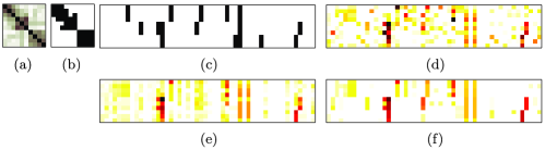
Figure 3: Regression coefficients estimated by different methods based on single simulated data. $b=0.8$ and threshold $\rho=0.3$ for the output correlation graph are used. Red pixels indicate large values. (a) The correlation coefficient matrix of phenotypes, (b) the edges of the phenotype correlation graph obtained at threshold 0.3 are shown as black pixels and (c) the true regression coefficients used in simulation. Absolute values of the estimated regression coefficients are shown for (d) lasso, (e) $\ell_{1}/\ell_{2}$ regularized multi-task regression and (f) graph-guided fused lasso. Rows correspond to outputs and columns to inputs.

$\beta_{ij}$ to a constant $b=0.8$ to construct the true coefficient matrix ${\mathbf{B}}$. Then, we simulate output data based on the linear regression model with noise distributed as standard Gaussian, using the simulated genotypes as inputs. We threshold the output correlation matrix in Figure 3(a) at $\rho=0.3$ to obtain the graph in Figure 3(b), and use this graph as prior structural information for the graph-guided fused lasso. As an illustrative example, the estimated regression coefficients from different regression models for recovering the association patterns are shown in Figures 3(d)–(f). While the results of the lasso and $\ell_{1}/\ell_{2}$-regularized multi-task regression with $\Omega({\mathbf{B}})=\sum_{j=1}^{J}\|{\bolds\beta}_{j,:}\|_{2}$ [Obozinski, Taskar and Jordan (2009)] in Figures 3(d) and (e) contain many false positives, the results from the graph-guided fused lasso in Figure 3(f) show fewer false positives and reveal clear block structures. Thus, the graph-guided fused lasso proves to be a superior regression model for recovering the true regression pattern that involves structured sparsity in the input/output relationships.

To compare SPG with FOBOS and IPM for QP in solving such a structured sparse regression problem, we vary $K$, $J$, $N$ and present the computation time in seconds in Figures 4(a)–(c), respectively. We select the regularization parameter $\gamma$ using separate validation data, and report the CPU time for the graph-guided fused lasso with the selected $\gamma$. The input/output data and true regression coefficient matrix ${\mathbf{B}}$

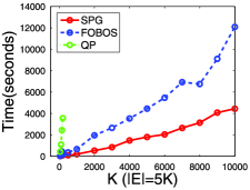
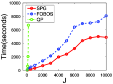
(a)	(b)
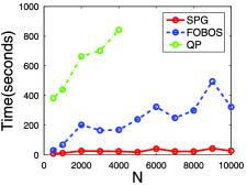
(c)

Figure 4: Comparisons of SPG, FOBOS and QP. (a) Vary $K$ from $50$ to $10\mbox{,}000$, fixing $N=500$, $J=100$; (b) vary $J$ from $50$ to $10\mbox{,}000$, fixing $N=1\mbox{,}000$, $K=50$; and (c) vary $N$ from $500$ to $10\mbox{,}000$, fixing $J=100$, $K=50$.

are generated in a way similar as above. More precisely, we assume that each group of correlated output variables is of size 10. For each group of the outputs, we randomly select $10\%$ of the input variables as relevant. In addition, we randomly select $5\%$ of the input variables as relevant to every two consecutive groups of outputs and $1\%$ of the input variables as relevant to every three consecutive groups. We set the $\rho$ for each data item so that the number of edges is 5 times the number of the nodes (i.e., $|E|=5K$). Figure 4 shows that SPG is substantially more efficient and can scale up to very high-dimensional and large-scale data sets. Moreover, we notice that the increase of $N$ almost does not affect the computation time of SPG, which is consistent with the complexity analysis in Section 3.5.

6.3 Real data analysis: Pathway analysis of breast cancer data

In this section we apply the SPG to an overlapping group lasso problem with a logistic loss on real-world data collected from breast cancer tumors [Jacob, Obozinski and Vert (2009), van de Vijver (2002)]. The main goal is to demonstrate the importance of employing structured sparsity-inducing penalties for performance enhancement in real life high-dimensional regression problems, thereby further exhibiting and justifying the needs of efficient solvers such as SPG for such problems.

The data are given as gene expression measurements for 8,141 genes in 295 breast-cancer tumors (78 metastatic and 217 nonmetastatic). A lot of research efforts in biology have been devoted to identifying biological pathways that consist of a group of genes participating in a particular biological process to perform a certain functionality in the cell. Thus, a powerful way of discovering genes involved in a tumor growth is to consider groups of interacting genes in each pathway rather than individual genes independently [Ma and Kosorok (2010)]. The overlapping-group-lasso penalty provides us with a natural way to incorporate this known pathway information into the biological analysis, where each group consists of the genes in each pathway. This approach can allow us to find pathway-level gene groups of significance that can distinguish the two tumor types. In our analysis of the breast cancer data, we cluster the genes using the canonical pathways from the Molecular Signatures Database [Subramanian et al. (2005)], and construct the overlapping-group-lasso penalty using the pathway-based clusters as groups. Many of the groups overlap because genes can participate in multiple pathways. Overall, we obtain 637 pathways over 3,510 genes, with each pathway containing 23.47 genes on average and each gene appearing in four pathways on average. Instead of analyzing all 8,141 genes, we focus on these 3,510 genes which belong to certain pathways. We set up the optimization problem of minimizing the logistic loss with the overlapping-group-lasso penalty to classify the tumor types based on the gene expression levels, and solve it with SPG.

Since the number of positive and negative samples are imbalanced, we adopt the balanced error rate defined as the average error rate of the two classes. We split the data into the training and testing sets with the ratio of $2:1$, and vary the $\lambda=\gamma$ from large to small to obtain the full regularization path.

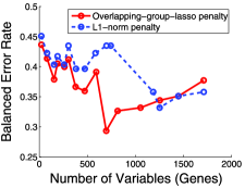
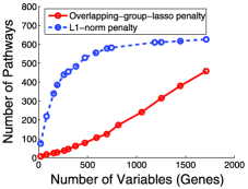
(a)	(b)

Figure 5: Results from the analysis of breast cancer data. (a) Balanced error rate for varying the number of selected genes, and (b) the number of pathways for varying the number of selected genes.

In Figure 5 we compare the results from fitting the logistic regression with the overlapping-group-lasso penalty with a baseline model with only the $\ell_{1}$-norm penalty. Figure 5(a) shows the balanced error rates for the different numbers of selected genes along the regularization path. As we can see, the balanced error rate for the model with the overlapping-group-lasso penalty is lower than the one with the $\ell_{1}$-norm, especially when the number of selected genes is between 500 to 1,000. The model with the overlapping-group-lasso penalty achieves the best error rate of 29.23% when 696 genes are selected, and these 696 genes belong to 125 different pathways. In Figure 5(b), for the different numbers of selected genes, we show the number of pathways to which the selected genes belong. From Figure 5(b) we see that when the group structure information is incorporated, fewer pathways are selected. This indicates that regression with the overlapping-group-lasso penalty selects the genes at the pathway level as a functionally coherent group, leading to an easy interpretation for functional analysis. On the other hand, the genes selected via the $\ell_{1}$-norm penalty are scattered across many pathways, as genes are considered independently for selection. The total computational time for computing the whole regularization path with 20 different values for the regularization parameters is 331 seconds for the overlapping group lasso.

We perform functional enrichment analysis on the selected pathways, using the functional annotation tool [Huang, Sherman and Lempicki (2009)], and verify that the selected pathways are significant in their relevance to the breast-cancer tumor types. For example, in a highly sparse model obtained with the group-lasso penalty at the very left end of Figure 5(b), the selected gene markers belong to only seven pathways, and many of these pathways appear to be reasonable candidates for an involvement in breast cancer. For instance, all proteins in one of the selected pathways are involved in the activity of proteases, whose function is to degrade unnecessary or damaged proteins through a chemical reaction that breaks peptide bonds. One of the most important malignant properties of cancer involves the uncontrolled growth of a group of cells, and protease inhibitors, which degrade misfolded proteins, have been extensively studied in the treatment of cancer. Another interesting pathway selected by the overlapping group lasso is known for its involvement in nicotinate and nicotinamide metabolism. This pathway has been confirmed as a marker for breast cancer in previous studies [Ma and Kosorok (2010)]. In particular, the gene ENPP1 (ectonucleotide pyrophosphatase/phosphodiesterase 1) in this pathway has been found to be overly expressed in breast tumors [Abate et al. (2005)]. Other selected pathways include the one related to ribosomes and another related to DNA polymerase, which are critical in the process of generating proteins from DNA and relevant to the property of uncontrolled growth in cancer cells.

We also examine the number of selected pathways that give the lowest error rate in Figure 5. At the error rate of 29.23%, 125 pathways (696 genes) are selected. It is interesting to notice that among these 125 pathways, one is closely related to apoptosis, which is the process of programmed cell death that occurs in multicellular organisms and is widely known to be involved in uncontrolled tumor growth in cancer. Another pathway involves the genes BRCA1, BRCA2 and ATR, which have all been associated with cancer susceptibility.

For comparison, we examine the genes selected with the $\ell_{1}$-norm penalty that does not consider the pathway information. In this case, we do not find any meaningful functional enrichment signals that are relevant to breast cancer. For example, among the 582 pathways that involve 687 genes at 37.55% error rate, we find two large pathways with functional enrichments, namely, response to organic substance (83 genes with $p$-value 3.3E$-$13) and the process of oxidation reduction (73 genes with $p$-value 1.7E$-$11). However, both are quite large groups and matched to relatively high-level biological processes that do not provide much insight on cancer-specific pathways.

7 Conclusions and future work

In this paper we investigated an optimization problem for estimating the structured-sparsity pattern in regression coefficients under a general class of structured sparsity-inducing penalties. Many of the structured sparsity-inducing penalties including the overlapping-group-lasso penalties and graph-guided-fused-lasso penalty share a common set of difficulties in optimization such as nonseparability and nonsmoothness. We showed that the optimization problems with these penalties can be transformed into a common form, and proposed a general optimization approach, called the smoothing proximal gradient method, for efficiently solving the optimization problem of this common form. Our results show that the proposed method enjoys both desirable theoretical guarantee and practical scalability under various difficult settings involving complex structure constraints, multi-task and high-dimensionality.

There are several future directions for this work. First, it is known that reducing $\mu$ over iterations leads to better empirical results. However, in such a scenario, the convergence rate is harder to analyze. Moreover, since the method is only based on gradient, its online version with the stochastic gradient descent can be easily derived. However, proving the regret bound will require a more careful investigation.

Another interesting direction is to incorporate other accelerating techniques into our method to further boost the performance. For example, the technique introduced in Zhou, Alexander and Lange (2011) can efficiently accelerate the algorithms which essentially solve a fixed point problem as ${\bolds\beta}=F({\bolds\beta})$. It uses an approximation of the Jacobian of $F({\bolds\beta})$. It is very interesting to incorporate this technique into our framework. However, since there is an $\ell_{1}$-norm penalty in our model and the operator $F$ is hence nondifferentiable, it is difficult to compute the approximation of the Jacobian of $F$. One potential strategy is to use the idea from the semi-smooth Newton method [Qi and Sun (1993), Sun, Womersley and Qi (2002)] to solve the nonsmooth operator $F$.

Appendix

.1 Proof of Theorem 1

We first introduce the concept of Fenchel conjugate.

Definition 1.

The Fenchel conjugate of a function $\varphi({\bolds\alpha})$ is the function $\varphi^{\ast}({\bolds\beta})$ defined as

$$\varphi^{\ast}({\bolds\beta})=\sup_{{\bolds\alpha}\in\operatorname{dom}(\varphi)}\bigl{(}{\bolds\alpha}^{T}{\bolds\beta}-\varphi({\bolds\alpha})\bigr{)}.$$

Recall that $d({\bolds\alpha})=\frac{1}{2}\|{\bolds\alpha}\|^{2}$ with the $\operatorname{dom}({\bolds\alpha})=\mathcal{Q}$. According to Definition 1, the conjugate of $d(\cdot)$ at $\frac{C{\bolds\beta}}{\mu}$ is $d^{\ast}(\frac{C{\bolds\beta}}{\mu})=\sup_{{\bolds\alpha}\in\mathcal{Q}}({\bolds\alpha}^{T}\frac{C{\bolds\beta}}{\mu}-d({\bolds\alpha}))$ and, hence,

$$f_{\mu}({\bolds\beta})\equiv\mathop{\arg\max}_{{\bolds\alpha}\in\mathcal{Q}}\bigl{(}{\bolds\alpha}^{T}C{\bolds\beta}-\mu d({\bolds\alpha})\bigr{)}=\mu d^{\ast}\biggl{(}\frac{C{\bolds\beta}}{\mu}\biggr{)}.$$

According to Theorem 26.3 in Rockafellar (1996), “a closed proper convex function is essentially strictly convex if and only if its conjugate is essentially smooth.” Since $d({\bolds\alpha})$ is a closely proper strictly convex function, its conjugate is smooth. Therefore, $f_{\mu}({\bolds\beta})$ is a smooth function.

Now we apply Danskin’s theorem [Proposition B.25 in Bertsekas (1999)] to derive $\nabla f_{\mu}({\bolds\beta})$. Let $\phi({\bolds\alpha},{\bolds\beta})={\bolds\alpha}^{T}C{\bolds\beta}-\mu\,d({\bolds\alpha})$. Since $d(\cdot)$ is a strongly convex function, $\mathop{\arg\max}_{{\bolds\alpha}\in\mathcal{Q}}\phi({\bolds\alpha},{\bolds\beta})$ has a unique optimal solution and we denote it as ${\bolds\alpha}^{\ast}$. According to Danskin’s theorem,

$$\nabla f_{\mu}({\bolds\beta})=\nabla_{{\bolds\beta}}\phi({\bolds\alpha}^{\ast},{\bolds\beta})=C^{T}{\bolds\alpha}^{\ast}.$$ (27)

As for the proof of the Lipschitz constant of $f_{\mu}({\bolds\beta})$, readers may refer to Nesterov (2005).

.2 Proof of Proposition 1

$${\bolds\alpha}^{\ast} = \mathop{\arg\max}_{{\bolds\alpha}\in\mathcal{Q}}\biggl{(}{\bolds\alpha}^{T}C{\bolds\beta}-\frac{\mu}{2}\|{\bolds\alpha}\|_{2}^{2}\biggr{)}$$

$$= \mathop{\arg\max}_{{\bolds\alpha}\in\mathcal{Q}}\sum_{g\in\mathcal{G}}\biggl{(}\gamma w_{g}{\bolds\alpha}_{g}^{T}{\bolds\beta}_{g}-\frac{\mu}{2}\|{\bolds\alpha}_{g}\|_{2}^{2}\biggr{)}$$

$$= \mathop{\arg\min}_{{\bolds\alpha}\in\mathcal{Q}}\sum_{g\in\mathcal{G}}\biggl{\|}{\bolds\alpha}_{g}-\frac{\gamma w_{g}{\bolds\beta}_{g}}{\mu}\biggr{\|}_{2}^{2}.$$

Therefore, (.2) can be decomposed into $|\mathcal{G}|$ independent problems: each one is the Euclidean projection onto the $\ell_{2}$-ball:

$${\bolds\alpha}^{\ast}_{g}=\mathop{\arg\min}_{{\bolds\alpha}_{g}\dvtx\|{\bolds\alpha}_{g}\|_{2}\leq 1}\biggl{\|}{\bolds\alpha}_{g}-\frac{\gamma w_{g}{\bolds\beta}_{g}}{\mu}\biggr{\|}_{2}^{2}$$

and ${\bolds\alpha}^{\ast}=[({\bolds\alpha}_{g_{1}}^{\ast})^{T},\ldots,({\bolds\alpha}_{g_{|\mathcal{G}|}}^{\ast})^{T}]^{T}$. According to the property of the $\ell_{2}$-ball, it can be easily shown that

$${\bolds\alpha}^{\ast}_{g}=S\biggl{(}\frac{\gamma w_{g}{\bolds\beta}_{g}}{\mu}\biggr{)},$$

where

$$S({\mathbf{u}})=\cases{\dfrac{{\mathbf{u}}}{\|{\mathbf{u}}\|_{2}},&\quad$\|{\mathbf{u}}\|_{2}>1$,\vspace*{2pt}\cr{\mathbf{u}},&\quad$\|{\mathbf{u}}\|_{2}\leq 1$.}$$

As for $\|C\|$,

$$\|C{\mathbf{v}}\|_{2}=\gamma\sqrt{\sum_{{g\in\mathcal{G}}}\sum_{j\in g}(w_{g})^{2}v_{j}^{2}}=\lambda\sqrt{\sum_{j=1}^{J}\biggl{(}\sum_{{g\in\mathcal{G}}\ \mathrm{s.t.}\ j\in g}(w_{g})^{2}\biggr{)}v_{j}^{2}},$$

the maximum value of $\|C{\mathbf{v}}\|_{2}$, given $\|{\mathbf{v}}\|_{2}\leq 1$, can be achieved by setting $v_{\hat{j}}$ for $j$ corresponding to the largest summation $\sum_{{g\in\mathcal{G}}\ \mathrm{s.t.}\ j\in g}(w_{g})^{2}$ to one, and setting other $v_{j}$’s to zeros. Hence, we have

$$\|C{\mathbf{v}}\|_{2}=\gamma\max_{j\in\{1,\ldots,J\}}\sqrt{\sum_{{g\in\mathcal{G}}\ \mathrm{s.t.}\ j\in g}(w_{g})^{2}}.$$

.3 Proof of Proposition 2

Similar to the proof technique of Proposition 1, we reformulate the problem of solving ${\bolds\alpha}^{\ast}$ as a Euclidean projection:

$${\bolds\alpha}^{\ast}=\mathop{\arg\max}_{{\bolds\alpha}\in\mathcal{Q}}\biggl{(}{\bolds\alpha}^{T}C{\bolds\beta}-\frac{\mu}{2}\|{\bolds\alpha}\|_{2}^{2}\biggr{)}=\mathop{\arg\min}_{{\bolds\alpha}\dvtx\|{\bolds\alpha}\|_{\infty}\leq 1}\biggl{\|}{\bolds\alpha}-\frac{C{\bolds\beta}}{\mu}\biggr{\|}_{2}^{2},$$

and the optimal solution ${\bolds\alpha}^{\ast}$ can be obtained by projecting $\frac{C{\bolds\beta}}{\mu}$ onto the $\ell_{\infty}$-ball.

According to the construction of the matrix $C$, we have, for any vector ${\mathbf{v}}$,

$$\|C{\mathbf{v}}\|_{2}^{2}=\gamma^{2}\sum_{e=(m,l)\in E}(\tau(r_{ml}))^{2}\bigl{(}v_{m}-\operatorname{sign}(r_{ml})v_{l}\bigr{)}^{2}.$$ (29)

By the simple fact that $(a\pm b)^{2}\leq 2a^{2}+2b^{2}$ and the inequality holds as equality if and only if $a=\pm b$, for each edge $e=(m,l)\in E$, the value $(v_{m}-\operatorname{sign}(r_{ml})v_{l})^{2}$ is upper bounded by $2v_{m}^{2}+2v_{l}^{2}$. Hence, when $\|{\mathbf{v}}\|_{2}=1$, the right-hand side of (29) can be further bounded by

$$\|C{\mathbf{v}}\|_{2}^{2} \leq \gamma^{2}\sum_{e=(m,l)\in E}2(\tau(r_{ml}))^{2}(v_{m}^{2}+v_{l}^{2})$$

$$= \gamma^{2}\sum_{j\in V}\biggl{(}\sum_{e\ \mathrm{incidenton}\ k}2(\tau(r_{e}))^{2}\biggr{)}v_{j}^{2}$$

$$= \gamma^{2}\sum_{j\in V}2d_{j}v_{j}^{2}$$

$$\leq 2\gamma^{2}\max_{j\in V}d_{j},$$

where

$$d_{j}=\sum_{e\in E\ \mathrm{s.t.}\ e\ \mathrm{incident}\ \mathrm{on}\ j}(\tau(r_{e}))^{2}.$$

Therefore, we have

$$\|C\|\equiv\max_{\|{\mathbf{v}}\|_{2}\leq 1}\|C{\mathbf{v}}\|_{2}\leq\sqrt{2\gamma^{2}\max_{j\in V}d_{j}}.$$

Note that this upper bound is tight because the first inequality in (.3) is tight.

.4 Proof of Theorem 2

Based on the result from Beck and Teboulle (2009), we have the following lemma:

Lemma 1

For the function $\widetilde{f}({\bolds\beta})=h({\bolds\beta})+\lambda\|{\bolds\beta}\|_{1}$, where $h({\bolds\beta})$ is an arbitrary convex smooth function and its gradient $\nabla h({\bolds\beta})$ is Lipschitz continuous with the Lipschitz constant $L$, we apply Algorithm 1 to minimize $\widetilde{f}({\bolds\beta})$ and let ${\bolds\beta}^{t}$ be the approximate solution at the $t$th iteration. For any ${\bolds\beta}$, we have the following bound:

$$\widetilde{f}({\bolds\beta}^{t})-\widetilde{f}({\bolds\beta})\leq\frac{2L\|{\bolds\beta}-{\bolds\beta}^{0}\|_{2}^{2}}{t^{2}}.$$ (31)

In order to use the bound in (31), we use the similar proof scheme as in Lan, Lu and Monteiro (2011) and decompose $f({\bolds\beta}^{t})-f({\bolds\beta}^{\ast})$ into three terms:

$$f({\bolds\beta}^{t})-f({\bolds\beta}^{\ast}) = \bigl{(}f({\bolds\beta}^{t})-\widetilde{f}({\bolds\beta}^{t})\bigr{)}+\bigl{(}\widetilde{f}({\bolds\beta}^{t})-\widetilde{f}({\bolds\beta}^{\ast})\bigr{)}$$

$${}+\bigl{(}\widetilde{f}({\bolds\beta}^{\ast})-f({\bolds\beta}^{\ast})\bigr{)}.$$

According to the definition of $\widetilde{f}$, we know that for any ${\bolds\beta}$

$$\widetilde{f}({\bolds\beta})\leq f({\bolds\beta})\leq\widetilde{f}({\bolds\beta})+\mu D,$$

where $D\equiv\max_{{\bolds\alpha}\in\mathcal{Q}}d({\bolds\alpha})$. Therefore, the first term in (.4), $f({\bolds\beta}^{t})-\widetilde{f}({\bolds\beta}^{t})$, is upper-bounded by $\mu D$, and the last term in (.4) is less than or equal to 0 [i.e., $\widetilde{f}({\bolds\beta}^{\ast})-f({\bolds\beta}^{\ast})\leq 0$]. Combining (31) with these two simple bounds, we have

$$f({\bolds\beta}^{t})-f({\bolds\beta}^{\ast}) \leq \mu D+\frac{2L\|{\bolds\beta}^{\ast}-{\bolds\beta}^{0}\|_{2}^{2}}{t^{2}}$$

$$\leq \mu D+\frac{2\|{\bolds\beta}^{\ast}-{\bolds\beta}^{0}\|_{2}^{2}}{t^{2}}\biggl{(}\lambda_{\max}({\mathbf{X}}^{T}{\mathbf{X}})+\frac{\|C\|^{2}}{\mu}\biggr{)}.$$

By setting $\mu=\frac{\varepsilon}{2D}$ and plugging this into the right-hand side of (.4), we obtain

$$f({\bolds\beta}^{t})-f({\bolds\beta}^{\ast})\leq\frac{\varepsilon}{2}+\frac{2\|{\bolds\beta}^{\ast}\|_{2}^{2}}{t^{2}}\biggl{(}\lambda_{\max}({\mathbf{X}}^{T}{\mathbf{X}})+\frac{2D\|C\|^{2}}{\varepsilon}\biggr{)}.$$ (34)

If we require the right-hand side of (34) to be equal to $\varepsilon$ and solve it for $t$, we obtain the bound of $t$ in (21).

References

- Abate et al. (2005) {barticle}[auto:STB—2011/12/07—13:41:22] \bauthor\bsnmAbate, \bfnmN.\binitsN., \bauthor\bsnmChandalia, \bfnmM.\binitsM., \bauthor\bsnmSatija, \bfnmP.\binitsP. and \bauthor\bsnmAdams-Huet, \bfnmB.\binitsB. \bsuffixet al. (\byear2005). \btitleEnpp1/pc-1 k121q polymorphism and genetic susceptibility to type 2 diabetes. \bjournalDiabetes \bvolume54 \bpages1027–1213. \bptokimsref \endbibitem
- Beck and Teboulle (2009) {barticle}[mr] \bauthor\bsnmBeck, \bfnmAmir\binitsA. and \bauthor\bsnmTeboulle, \bfnmMarc\binitsM. (\byear2009). \btitleA fast iterative shrinkage-thresholding algorithm for linear inverse problems. \bjournalSIAM J. Imaging Sci. \bvolume2 \bpages183–202. \bidissn=1936-4954, mr=2486527 \bptokimsref \endbibitem
- Bertsekas (1999) {bbook}[auto:STB—2011/12/07—13:41:22] \bauthor\bsnmBertsekas, \bfnmD.\binitsD. (\byear1999). \btitleNonlinear Programming. \bpublisherAthena Scientific, \baddressNashua, NH. \bptokimsref \endbibitem
- Duchi and Singer (2009) {barticle}[mr] \bauthor\bsnmDuchi, \bfnmJohn\binitsJ. and \bauthor\bsnmSinger, \bfnmYoram\binitsY. (\byear2009). \btitleEfficient online and batch learning using forward backward splitting. \bjournalJ. Mach. Learn. Res. \bvolume10 \bpages2899–2934. \bidissn=1532-4435, mr=2579916 \bptokimsref \endbibitem
- Friedman, Hastie and Tibshirani (2010) {bmisc}[auto:STB—2011/12/07—13:41:22] \bauthor\bsnmFriedman, \bfnmJ.\binitsJ., \bauthor\bsnmHastie, \bfnmT.\binitsT. and \bauthor\bsnmTibshirani, \bfnmR.\binitsR. (\byear2010). \bhowpublishedA note on the group lasso and a sparse group lasso. Dept. Statistics, Stanford Univ. \bptokimsref \endbibitem
- Friedman et al. (2007) {barticle}[mr] \bauthor\bsnmFriedman, \bfnmJerome\binitsJ., \bauthor\bsnmHastie, \bfnmTrevor\binitsT., \bauthor\bsnmHöfling, \bfnmHolger\binitsH. and \bauthor\bsnmTibshirani, \bfnmRobert\binitsR. (\byear2007). \btitlePathwise coordinate optimization. \bjournalAnn. Appl. Stat. \bvolume1 \bpages302–332. \biddoi=10.1214/07-AOAS131, issn=1932-6157, mr=2415737 \bptokimsref \endbibitem
- Huang, Sherman and Lempicki (2009) {barticle}[auto:STB—2011/12/07—13:41:22] \bauthor\bsnmHuang, \bfnmD. W.\binitsD. W., \bauthor\bsnmSherman, \bfnmB. T.\binitsB. T. and \bauthor\bsnmLempicki, \bfnmR. A.\binitsR. A. (\byear2009). \btitleSystematic and integrative analysis of large gene lists using david bioinformatics resources. \bjournalNature Protoc. \bvolume4 \bpages44–57. \bptokimsref \endbibitem
- Jacob, Obozinski and Vert (2009) {bincollection}[auto:STB—2011/12/07—13:41:22] \bauthor\bsnmJacob, \bfnmL.\binitsL., \bauthor\bsnmObozinski, \bfnmG.\binitsG. and \bauthor\bsnmVert, \bfnmJ. P.\binitsJ. P. (\byear2009). \btitleGroup lasso with overlap and graph lasso. In \bbooktitleProceedings of the International Conference on Machine Learning. \bpublisherACM, \baddressMontreal, QC. \bptokimsref \endbibitem
- Jenatton, Audibert and Bach (2009) {bmisc}[auto:STB—2011/12/07—13:41:22] \bauthor\bsnmJenatton, \bfnmR.\binitsR., \bauthor\bsnmAudibert, \bfnmJ. Y.\binitsJ. Y. and \bauthor\bsnmBach, \bfnmF.\binitsF. (\byear2009). \bhowpublishedStructured variable selection with sparsity-inducing norms. Technical report, INRIA. \bptokimsref \endbibitem
- Jenatton et al. (2010) {bincollection}[auto:STB—2011/12/07—13:41:22] \bauthor\bsnmJenatton, \bfnmR.\binitsR., \bauthor\bsnmMairal, \bfnmJ.\binitsJ., \bauthor\bsnmObozinski, \bfnmG.\binitsG. and \bauthor\bsnmBach, \bfnmF.\binitsF. (\byear2010). \btitleProximal methods for sparse hierarchical dictionary learning. In \bbooktitleProceedings of the International Conference on Machine Learning. \bpublisherOmnipress, \baddressHaifa. \bptokimsref \endbibitem
- Kim, Sohn and Xing (2009) {barticle}[auto:STB—2011/12/07—13:41:22] \bauthor\bsnmKim, \bfnmS.\binitsS., \bauthor\bsnmSohn, \bfnmK. A.\binitsK. A. and \bauthor\bsnmXing, \bfnmE. P.\binitsE. P. (\byear2009). \btitleA multivariate regression approach to association analysis of a quantitative trait network. \bjournalBioinformatics \bvolume25 \bpages204–212. \bptokimsref \endbibitem
- Kim and Xing (2009) {barticle}[pbm] \bauthor\bsnmKim, \bfnmSeyoung\binitsS. and \bauthor\bsnmXing, \bfnmEric P.\binitsE. P. (\byear2009). \btitleStatistical estimation of correlated genome associations to a quantitative trait network. \bjournalPLoS Genet. \bvolume5 \bpagese1000587. \biddoi=10.1371/journal.pgen.1000587, issn=1553-7404, pmcid=2719086, pmid=19680538 \bptokimsref \endbibitem
- Kim and Xing (2010) {bincollection}[auto:STB—2011/12/07—13:41:22] \bauthor\bsnmKim, \bfnmS.\binitsS. and \bauthor\bsnmXing, \bfnmE. P.\binitsE. P. (\byear2010). \btitleTree-guided group lasso for multi-task regression with structured sparsity. In \bbooktitleProceedings of the International Conference on Machine Learning. \bpublisherOmnipress, \baddressHaifa. \bptokimsref \endbibitem
- Lan, Lu and Monteiro (2011) {barticle}[auto:STB—2011/12/07—13:41:22] \bauthor\bsnmLan, \bfnmG.\binitsG., \bauthor\bsnmLu, \bfnmZ.\binitsZ. and \bauthor\bsnmMonteiro, \bfnmR.\binitsR. (\byear2011). \btitlePrimal-dual first-order methods with iteration complexity for cone programming. \bjournalMathematical Programming \bvolume126 \bpages1–29. \bptokimsref \endbibitem
- Lange (2004) {bbook}[auto:STB—2011/12/07—13:41:22] \bauthor\bsnmLange, \bfnmK.\binitsK. (\byear2004). \btitleOptimization. \bpublisherSpringer, \baddressBerlin. \bptokimsref \endbibitem
- Liu, Ji and Ye (2009) {bincollection}[auto:STB—2011/12/07—13:41:22] \bauthor\bsnmLiu, \bfnmJ.\binitsJ., \bauthor\bsnmJi, \bfnmS.\binitsS. and \bauthor\bsnmYe, \bfnmJ.\binitsJ. (\byear2009). \btitleMulti-task feature learning via efficient -norm minimization. In \bbooktitleProceedings of the Uncertainty in AI. \bpublisherAUAI Press, \baddressMontreal, QC. \bptokimsref \endbibitem
- Liu and Ye (2010a) {bmisc}[auto:STB—2011/12/07—13:41:22] \bauthor\bsnmLiu, \bfnmJ.\binitsJ. and \bauthor\bsnmYe, \bfnmJ.\binitsJ. (\byear2010a). \bhowpublishedFast overlapping group lasso. Available at arXiv:1009.0306v1. \bptokimsref \endbibitem
- Liu and Ye (2010b) {bincollection}[auto:STB—2011/12/07—13:41:22] \bauthor\bsnmLiu, \bfnmJ.\binitsJ. and \bauthor\bsnmYe, \bfnmJ.\binitsJ. (\byear2010b). \btitleMoreau-yosida regularization for grouped tree structure learning. In \bbooktitleAdvances in Neural Information Processing Systems (NIPS). \bpublisherCurran Associates, Inc., \baddressVancouver, BC. \bptokimsref \endbibitem
- Liu, Yuan and Ye (2010) {bincollection}[auto:STB—2011/12/07—13:41:22] \bauthor\bsnmLiu, \bfnmJ.\binitsJ., \bauthor\bsnmYuan, \bfnmL.\binitsL. and \bauthor\bsnmYe, \bfnmJ.\binitsJ. (\byear2010). \btitleAn efficient algorithm for a class of fused lasso problems. In \bbooktitleThe ACM SIG Knowledge Discovery and Data Mining. \bpublisherACM, \baddressWashington, DC. \bptokimsref \endbibitem
- Ma and Kosorok (2010) {barticle}[pbm] \bauthor\bsnmMa, \bfnmShuangge\binitsS. and \bauthor\bsnmKosorok, \bfnmMichael R.\binitsM. R. (\byear2010). \btitleDetection of gene pathways with predictive power for breast cancer prognosis. \bjournalBMC Bioinformatics \bvolume11 \bpages1. \biddoi=10.1186/1471-2105-11-1, issn=1471-2105, pii=1471-2105-11-1, pmcid=2837025, pmid=20043860 \bptokimsref \endbibitem
- Mairal et al. (2010) {bincollection}[auto:STB—2011/12/07—13:41:22] \bauthor\bsnmMairal, \bfnmJ.\binitsJ., \bauthor\bsnmJenatton, \bfnmR.\binitsR., \bauthor\bsnmObozinski, \bfnmG.\binitsG. and \bauthor\bsnmBach, \bfnmF.\binitsF. (\byear2010). \btitleNetwork flow algorithms for structured sparsity. In \bbooktitleAdvances in Neural Information Processing Systems (NIPS). \bpublisherCurran Associates, Inc., \baddressVancouver, BC. \bptokimsref \endbibitem
- Nesterov (2003) {bmisc}[auto:STB—2011/12/07—13:41:22] \bauthor\bsnmNesterov, \bfnmY.\binitsY. (\byear2003). \bhowpublishedExcessive gap technique in non-smooth convex minimization. Technical report, Univ. Catholique de Louvain, Center for Operations Research and Econometrics (CORE). \bptokimsref \endbibitem
- Nesterov (2005) {barticle}[auto:STB—2011/12/07—13:41:22] \bauthor\bsnmNesterov, \bfnmY.\binitsY. (\byear2005). \btitleSmooth minimization of non-smooth functions. \bjournalMathematical Programming \bvolume103 \bpages127–152. \bptokimsref \endbibitem
- Nesterov (2007) {bmisc}[auto:STB—2011/12/07—13:41:22] \bauthor\bsnmNesterov, \bfnmY.\binitsY. (\byear2007). \bhowpublishedGradient methods for minimizing composite objective function. ECORE Discussion Paper 2007. \bptokimsref \endbibitem
- Obozinski, Taskar and Jordan (2009) {bincollection}[auto:STB—2011/12/07—13:41:22] \bauthor\bsnmObozinski, \bfnmG.\binitsG., \bauthor\bsnmTaskar, \bfnmB.\binitsB. and \bauthor\bsnmJordan, \bfnmM. I.\binitsM. I. (\byear2009). \btitleHigh-dimensional union support recovery in multivariate regression. In \bbooktitleAdvances in Neural Information Processing Systems (NIPS). \bpublisherCurran Associates, Inc., \baddressVancouver, BC. \bptokimsref \endbibitem
- Qi and Sun (1993) {barticle}[auto:STB—2011/12/07—13:41:22] \bauthor\bsnmQi, \bfnmL.\binitsL. and \bauthor\bsnmSun, \bfnmJ.\binitsJ. (\byear1993). \btitleA nonsmooth version of newton’s method. \bjournalMathematical Programming \bvolume58 \bpages353–367. \bptokimsref \endbibitem
- Rockafellar (1996) {bbook}[auto:STB—2011/12/07—13:41:22] \bauthor\bsnmRockafellar, \bfnmR.\binitsR. (\byear1996). \btitleConvex Analysis. \bpublisherPrinceton Univ. Press, \baddressPrinceton. \bptokimsref \endbibitem
- Subramanian et al. (2005) {barticle}[auto:STB—2011/12/07—13:41:22] \bauthor\bsnmSubramanian, \bfnmA.\binitsA., \bauthor\bsnmTamayo, \bfnmP.\binitsP. and \bauthor\bsnmMootha, \bfnmV.\binitsV. \bsuffixet al. (\byear2005). \btitleGene set enrichment analysis: A knowledge-based approach for interpreting genome-wide expression profiles. \bjournalProc. Natl. Acad. Sci. USA \bvolume102 \bpages15545–15550. \bptokimsref \endbibitem
- Sun, Womersley and Qi (2002) {barticle}[auto:STB—2011/12/07—13:41:22] \bauthor\bsnmSun, \bfnmD.\binitsD., \bauthor\bsnmWomersley, \bfnmR.\binitsR. and \bauthor\bsnmQi, \bfnmH.\binitsH. (\byear2002). \btitleA feasible semismooth asymptotically Newton method for mixed complementarity problems. \bjournalMathematical Programming, Ser. A \bvolume94 \bpages167–187. \bptokimsref \endbibitem
- The International HapMap Consortium (2005) {bmisc}[auto:STB—2011/12/07—13:41:22] \borganizationThe International HapMap Consortium. (\byear2005). \bhowpublishedA haplotype map of the human genome. Nature 437 1399–1320. \bptokimsref \endbibitem
- Tibshirani (1996) {barticle}[auto:STB—2011/12/07—13:41:22] \bauthor\bsnmTibshirani, \bfnmR.\binitsR. (\byear1996). \btitleRegression shrinkage and selection via the lasso. \bjournalJ. R. Stat. Soc. Ser. B \bvolume58 \bpages267–288. \bidmr=1379242 \bptokimsref \endbibitem
- Tibshirani and Saunders (2005) {barticle}[auto:STB—2011/12/07—13:41:22] \bauthor\bsnmTibshirani, \bfnmR.\binitsR. and \bauthor\bsnmSaunders, \bfnmM.\binitsM. (\byear2005). \btitleSparsity and smoothness via the fused lasso. \bjournalJ. R. Stat. Soc. Ser. B Stat. Methodol. \bvolume67 \bpages91–108. \bidmr=2136641 \bptokimsref \endbibitem
- Tibshirani and Taylor (2010) {barticle}[auto:STB—2011/12/07—13:41:22] \bauthor\bsnmTibshirani, \bfnmR.\binitsR. and \bauthor\bsnmTaylor, \bfnmJ.\binitsJ. (\byear2010). \btitleThe solution path of the generalized lasso. \bjournalAnn. Statist. \bvolume39 \bpages1335–1371. \bidmr=2850205 \bptokimsref \endbibitem
- Tseng (2008) {bmisc}[auto:STB—2011/12/07—13:41:22] \bauthor\bsnmTseng, \bfnmP.\binitsP. (\byear2008). \bhowpublishedOn accelerated proximal gradient methods for convex-concave optimization. SIAM J. Optim. To appear. \bptokimsref \endbibitem
- Tütüncü, Toh and Todd (2003) {barticle}[auto:STB—2011/12/07—13:41:22] \bauthor\bsnmTütüncü, \bfnmR. H.\binitsR. H., \bauthor\bsnmToh, \bfnmK. C.\binitsK. C. and \bauthor\bsnmTodd, \bfnmM. J.\binitsM. J. (\byear2003). \btitleSolving semidefinite-quadratic-linear programs using sdpt3. \bjournalMathematical Programming \bvolume95 \bpages189–217. \bptokimsref \endbibitem
- van de Vijver (2002) {barticle}[auto:STB—2011/12/07—13:41:22] \bauthor\bparticlevan de \bsnmVijver, \bfnmM. J.\binitsM. J. \bsuffixet al. (\byear2002). \btitleA gene-expression signature as a predictor of survival in breast cancer. \bjournalNew England Journal of Medicine \bvolume347 \bpages1999–2009. \bptokimsref \endbibitem
- Wu and Lange (2008) {barticle}[auto:STB—2011/12/07—13:41:22] \bauthor\bsnmWu, \bfnmT.\binitsT. and \bauthor\bsnmLange, \bfnmK.\binitsK. (\byear2008). \btitleCoordinate descent algorithms for lasso penalized regression. \bjournalAnn. Appl. Stat. \bvolume2 \bpages224–244. \bidmr=2415601 \bptokimsref \endbibitem
- Yuan and Lin (2006) {barticle}[auto:STB—2011/12/07—13:41:22] \bauthor\bsnmYuan, \bfnmM.\binitsM. and \bauthor\bsnmLin, \bfnmY.\binitsY. (\byear2006). \btitleModel selection and estimation in regression with grouped variables. \bjournalJ. R. Stat. Soc. Ser. B Stat. Methodol. \bvolume68 \bpages49–67. \bidmr=2212574 \bptokimsref \endbibitem
- Zhang et al. (2010) {barticle}[pbm] \bauthor\bsnmZhang, \bfnmZhongyang\binitsZ., \bauthor\bsnmLange, \bfnmKenneth\binitsK., \bauthor\bsnmOphoff, \bfnmRoel\binitsR. and \bauthor\bsnmSabatti, \bfnmChiara\binitsC. (\byear2010). \btitleReconstructing DNA copy number by penalized estimation and imputation. \bjournalAnn. Appl. Stat. \bvolume4 \bpages1749–1773. \biddoi=10.1214/10-AOAS357, issn=1941-7330, mid=NIHMS288657, pmcid=3092301, pmid=21572975, mr=2829935 \bptokimsref \endbibitem
- Zhao, Rocha and Yu (2009a) {barticle}[auto:STB—2011/12/07—13:41:22] \bauthor\bsnmZhao, \bfnmP.\binitsP., \bauthor\bsnmRocha, \bfnmG.\binitsG. and \bauthor\bsnmYu, \bfnmB.\binitsB. (\byear2009a). \btitleThe composite absolute penalties family for grouped and hierarchical variable selection. \bjournalAnn. Statist. \bvolume37 \bpages3468–3497. \bidmr=2549566 \bptokimsref \endbibitem
- Zhao, Rocha and Yu (2009b) {barticle}[auto:STB—2011/12/07—13:41:22] \bauthor\bsnmZhao, \bfnmP.\binitsP., \bauthor\bsnmRocha, \bfnmG.\binitsG. and \bauthor\bsnmYu, \bfnmB.\binitsB. (\byear2009b). \btitleGrouped and hierarchical model selection through composite absolute penalties. \bjournalAnn. Statist. \bvolume37 \bpages3468–3497. \bptokimsref \endbibitem
- Zhou, Alexander and Lange (2011) {barticle}[pbm] \bauthor\bsnmZhou, \bfnmHua\binitsH., \bauthor\bsnmAlexander, \bfnmDavid\binitsD. and \bauthor\bsnmLange, \bfnmKenneth\binitsK. (\byear2011). \btitleA quasi-Newton acceleration for high-dimensional optimization algorithms. \bjournalStat. Comput. \bvolume21 \bpages261–273. \biddoi=10.1007/s11222-009-9166-3, issn=0960-3174, mid=NIHMS205483, pmcid=3045213, pmid=21359052, mr=2774856 \bptokimsref \endbibitem
- Zhou and Lange (2011) {bmisc}[auto:STB—2011/12/07—13:41:22] \bauthor\bsnmZhou, \bfnmH.\binitsH. and \bauthor\bsnmLange, \bfnmK.\binitsK. (\byear2011). \bhowpublishedA path algorithm for constrained estimation. Available at arXiv:1103.3738v1. \bptokimsref \endbibitem