Out-of-equilibrium heating of electron liquid: fermionic and bosonic temperatures

Abstract

We investigate out-of-the equilibrium properties of the electron liquid in a two-dimensional disordered superconductor subject to the electric bias and temperature gradient. We calculate kinetic coefficients and Nyquist noise, and find that they are characterized by distinct effective temperatures: $T_{\mathrm{e}}$, characterizing single-particle excitations, $T_{\mathrm{Cp}}$, describing the Cooper pairs, and $T_{\mathrm{eh}}$, corresponding to electron-hole or dipole excitations. Varying the ratio between the electric $j$ and thermal $j_{\mathrm{th}}$ currents and boundary conditions one can heat different kind of excitations tuning their corresponding temperatures. We propose the experiment to determine these effective temperatures.

A temperature, the term quantifying the common idea of “hot” and “cold,” is one of the most fundamental concepts in physics. In statistical physics, the temperature is a parameter that controls the probability of the energy distribution of a given system over the possible states. The basic property of the temperature is that in an equilibrium it is the constant all over the system involved due to the interactions between the constituent subsystems. In out of the equilibrium case, different subsystems can acquire different temperatures. Electrons and phonons which equilibrate within themselves, but can possess different temperatures if weakly coupled, is an exemplary case of such a non-equilibrium situation Giazotto ; Volkov_Kogan .

In this Letter we show that strong correlations bring more richness to the non-equilibrium physics. We construct a kinetic theory of electronic transport in a disordered two-dimensional (2D) superconductor and demonstrate that distinct electronic subsystems respond differently to external drive. We derive transport kinetic coefficients and find that they are controlled by distinctive effective fermionic and bosonic temperatures each corresponding to a particular electronic subsystems: $T_{\mathrm{e}}$ for the single-particle excitations, $T_{\mathrm{\scriptscriptstyle Cp}}$ for Cooper pairs, and $T_{\mathrm{eh}}$ for electron-hole pairs (dipoles). These temperatures are defined through the respective energy distribution functions, and the relations between them are determined by the character of the external drive, or more specifically, by the ratio of its components, the applied voltage bias and/or temperature gradient (see Fig. 1).

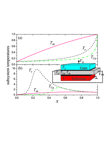
Figure 1: Temperatures of electron-hole pairs ($T_{\mathrm{eh}}$), Cooper pairs ($T_{\mathrm{\scriptscriptstyle Cp}}$) and quasi-particles ($T_{\mathrm{e}}$) vs. the parameter $x=R_{2}/(R_{1}+R_{2})$, characterizing the ratio between tunneling resistances $R_{1}$ between the substrate and superconducting film and $R_{2}$, between the film and the gate. The substrate temperature is $T_{1}$ and the gate temperature is $T_{2}$, $T_{2}/T_{1}=0.1$, the voltage drop between them is $V_{\scriptscriptstyle G}$. (a) $V_{\scriptscriptstyle G}=0$, where only thermal current is present; (b) $eV_{\scriptscriptstyle G}/T_{1}=3$, with $V_{G}j\gtrsim j_{\mathrm{th}}$.
Generally, in the film driven far from equilibrium and for $R_{1}\simeq R_{2}$, different interrelations between fermionic and bosonic temperatures can be realized: $T_{\mathrm{e}}\simeq T_{\mathrm{\scriptscriptstyle Cp}}\ll T_{\mathrm{eh}}$ for $j_{\mathrm{th}}\gg V_{\scriptscriptstyle G}j$, while $T_{\mathrm{e}}\simeq T_{\mathrm{Cp}}\gg T_{\mathrm{eh}}$ for $j_{\mathrm{th}}\ll V_{\scriptscriptstyle G}j$.

We consider 2D disordered systems such that the Thouless energy corresponding to diffusion across the film $E_{T}^{\perp}=D/d^{2}$, where $D$ is the diffusion coefficient, $d$ is the film thickness, well exceeds all the fermionic and bosonic temperatures. Hereafter we will use units where $k_{B}=\hbar=c=1$ ($c$ is the light velocity). The bias-dependent subsystem temperatures manifest themselves most profoundly in the leading quantum corrections Varlamov_book to the sheet conductance in the singlet, $\delta G^{\mathrm{\scriptscriptstyle AA}}$ (Aronov-Altshuler correction) and in the Copper channel, $\delta G^{\mathrm{\scriptscriptstyle MT}}$ (Maki-Thomson correction) close to the transition:

$$\delta G^{\mathrm{\scriptscriptstyle AA}} =\frac{e^{2}}{2\pi^{2}}\ln({T_{\mathrm{eh}}\tau})\,,$$ (1)

$$\delta G^{\mathrm{\scriptscriptstyle MT}} =\frac{e^{2}}{\pi}{T_{\mathrm{\scriptscriptstyle Cp}}\tau_{\mathrm{\scriptscriptstyle GL}}}\ln{\left(\tau_{\phi}/\tau_{\mathrm{\scriptscriptstyle GL}}\right)},$$ (2)

and in the leading contribution to the in-plane Nyquist noise,

$$S_{\mathrm{th}}(\omega=0)\approx 2\sigma_{\mathrm{\scriptscriptstyle D}}T_{\mathrm{eh}}.$$ (3)

Here $e$ is the electron charge, $\tau$ is the elastic scattering time, $\tau_{\phi}$ is the dephasing time, $\tau_{\mathrm{\scriptscriptstyle GL}}$ is the Ginzburg-Landau time indicating how close the system is to the superconducting transition, and $\sigma_{\mathrm{\scriptscriptstyle D}}$ is the Drude conductivity. We consider disordered system where $T_{\mathrm{eh({\scriptscriptstyle Cp})}}\ll\tau^{-1}$, $e^{2}/(\sigma_{\mathrm{\scriptscriptstyle D}}d)\ll 1$, and $\tau_{\mathrm{\scriptscriptstyle GL}}\ll\tau_{\phi}$.

The fermionic and bosonic temperatures are defined through the respective distribution functions, that are assumed to be space and time independent. We start with the fermionic temperature $T_{\mathrm{e}}$ describing the low lying single-particle excitations. In an equilibrium, the electron (hole) gauge invariant distribution function in the disordered electron liquid is $\tilde{f}_{\mathrm{e(h)}}^{\mathrm{(eq)}}(\epsilon)=f_{\mathrm{\scriptscriptstyle F}}(\epsilon)\equiv 1/[\exp(\epsilon/T)+1]$, where $\epsilon$ is the quasiparticle energy, and the temperature appears as its low-energy “cut-off”: $T=\epsilon/2[1-2\tilde{f}_{\mathrm{e(h)}}^{\mathrm{(eq)}}(\epsilon)]|_{\epsilon\to 0}$. Generalizing onto an out of the equilibrium case, one arrives at:

$$T_{\mathrm{e}}=\{-4\lim_{\epsilon\to 0}\partial_{\epsilon}\tilde{f}_{\mathrm{\scriptscriptstyle L}}(\epsilon)\}^{-1},$$ (4)

where $\tilde{f}_{\mathrm{\scriptscriptstyle L}}(\epsilon)=[\tilde{f}_{\mathrm{e}}(\epsilon)+\tilde{f}_{\mathrm{h}}(\epsilon)]/2$, and $\tilde{f}_{\mathrm{e(h)}}(\epsilon)$ is a general nonequilibrium electron (hole) distribution function.

The electron-hole ($e$-$h$) pair temperature $T_{\mathrm{eh}}$ emerges in the bosonic distribution function of the electron-hole excitations mediating, for example, the electronic transport in metals CVB . The bosonic nature of the $e$-$h$ environment is revealed by the fluctuation-dissipation theorem (FDT) for the density-density correlation function in a quasi-equilibrium regime: $\Pi^{K}(\mathbf{q},\omega)=2i(1+2N^{\rm(eq)}_{\omega})\operatorname{Im}\Pi^{R}(\omega,\mathbf{q})$, where $N^{\rm(eq)}_{\omega}$ is the Bose distribution function of the $e$-$h$ excitations, $\Pi^{R}(x-y)$ is the retarded correlator of the electron density, and $\Pi^{K}(x-y)$ is the Keldysh density correlator. The low-energy cut-off of the distribution function $N^{\rm(eq)}$ defines $T_{\mathrm{eh}}=\omega N^{\rm(eq)}_{\omega}|_{\omega\to 0}$. In the nonequilibrium case we find

$$T_{\mathrm{eh}}=\lim_{\omega\to 0}\omega N_{\omega},$$ (5)

$$N_{\omega}=\frac{1}{2\omega}\sum_{\alpha=e,h}\int[1-\tilde{f}_{\alpha}(\epsilon_{-})]\tilde{f}_{\alpha}(\epsilon_{+})d\epsilon,$$ (6)

where $\epsilon_{\pm}=\epsilon\pm\omega/2$. The integrand in (6) gives the probability for the state with the energy $\epsilon_{+}$ be occupied and the state with the energy $\epsilon_{-}$ be empty. In an equilibrium $N_{\omega}\to N^{\rm(eq)}_{\omega}$.

Turning to the nonequilibrium generalization of the FDT in the Cooper channel, i.e. taking the Keldysh component of the fluctuation propagators in the Cooper channel, one arrives at the temperature for the fluctuating Cooper pairs as

$$T_{\mathrm{\scriptscriptstyle\scriptscriptstyle Cp}}=2T_{\mathrm{e}}z_{\mathrm{\scriptscriptstyle Cp}}\left\{\tilde{f}_{\mathrm{e}}(0)[1-\tilde{f}_{\mathrm{h}}(0)]+\tilde{f}_{\mathrm{h}}(0)[1-\tilde{f}_{\mathrm{e}}(0)]\right\}.$$ (7)

Here $z_{\mathrm{Cp}}=(1+(T_{\mathrm{e}}/\Omega)^{2})^{-1}$ and $\Omega^{-1}=4\mathchoice{{\vbox{\hbox{$\textstyle-$}}\kern-5.34723pt}}{{\vbox{\hbox{$\scriptstyle-$}}\kern-3.57503pt}}{{\vbox{\hbox{$\scriptscriptstyle-$}}\kern-2.52084pt}}{{\vbox{\hbox{$\scriptscriptstyle-$}}\kern-2.0625pt}}\!\int_{\epsilon}[\tilde{f}_{\mathrm{\scriptscriptstyle R}}(0)-\tilde{f}_{\mathrm{\scriptscriptstyle R}}(\epsilon)]/\pi\epsilon^{2}$, where $\tilde{f}_{\mathrm{\scriptscriptstyle R}}(\epsilon)=\tilde{f}_{\mathrm{e}}(-\epsilon)-\tilde{f}_{\mathrm{h}}(\epsilon)$. In an equilibrium $T_{\mathrm{e}}=T$, $z_{\mathrm{\scriptscriptstyle Cp}}=1$, $f_{\scriptscriptstyle{\mathrm{F}}}(0)[1-f_{\mathrm{\scriptscriptstyle F}}(0)]=1/4$, and therefore $T_{\mathrm{\scriptscriptstyle Cp}}=T$. The combination of distribution functions appearing in the definition of $T_{\mathrm{\scriptscriptstyle Cp}}$ can be viewed as the probability for generating a Cooper pair.

We consider a setup shown in Fig. 1, where the superconducting film is sandwiched between the substrate and the gate and is separated from them by the tunnel barriers with the resistances $R_{1}$ and $R_{2}$, respectively. We can manipulate the density matrix of the system applying the gate bias, $V_{\scriptscriptstyle G}$, and changing the temperatures $T_{1}$ and $T_{2}$ of the substrate and the gate. The electronic distribution functions defining the subsystem temperatures in the film are found from the respective kinetic equations. The thickness of the superconducting film $d$ is much smaller than the inelastic quasiparticle scattering length, thus the corresponding collision integral can be omitted. Then the kinetic equations in the stationary situation assume the form of the current conservation law, ${\boldsymbol{\nabla}}\mathbf{j}_{\mathrm{e(h)}}(\epsilon)=0$, where the spectral quasiparticle current $\mathbf{j}_{\mathrm{e(h)}}(\epsilon)=-D{\boldsymbol{\nabla}}f_{\mathrm{e(h)}}$. Here we use the gauge where $\mathbf{A}=0$. The boundary conditions require the conservation of $\mathbf{j}_{\mathrm{e(h)}}(\epsilon)$ and imply that $\mathbf{j}_{\mathrm{e(h)}}(\epsilon)=[f_{\mathrm{e(h)}}^{(f)}(\epsilon)-f_{\mathrm{e(h)}}^{(s)}(\epsilon)]/\nu e^{2}R_{1}$, where the indexes $s$ and $f$ denote substrate and film, respectively, and $\nu$ is the single-particle density of states at the Fermi level per spin projection Kuprianov+ . Similar relation holds for $\mathbf{j}_{\mathrm{e(h)}}(\epsilon)$ between the film and the gate. The gauge invariant distribution functions satisfy the kinetic equations which contain directly the electromagnetic fields rather then their respective potentials. In our case electric field enters the kinetic equation through the boundary conditions. In order to obtain the gauge-invariant distribution functions, one uses the transformation $\tilde{f}_{\mathrm{e(h)}}(\epsilon)=f_{\mathrm{e(h)}}(\epsilon\pm e\phi_{{\mathrm{f}}})$, where $\phi_{{\mathrm{f}}}$ is the electric potential in the film, see, e.g., Rammer-Smith ; Kopnin_book . Thus,

$$\tilde{f}_{\mathrm{e(h)}}(\epsilon)=xf_{\mathrm{\scriptscriptstyle F}}\left({\epsilon\pm eV_{\scriptscriptstyle G}(1-x)},{T_{1}}\right)+\\ (1-x)f_{\mathrm{\scriptscriptstyle F}}\left({\epsilon\mp eV_{\scriptscriptstyle G}x},{T_{2}}\right),$$ (8)

where the temperature appears as the second argument in the Fermi-functions, and $x=R_{2}/R_{\scriptsize{\scriptscriptstyle\Sigma}}$ with $R_{\scriptscriptstyle\Sigma}=R_{1}+R_{2}$. Expressing subsystem temperatures through the contact parameters and using definitions Eqs.(4)-(5), one finds:

$$\begin{split}T_{\mathrm{eh}}\approx x^{2}T_{1}+(&1-x)^{2}T_{2}+\\ &x(1-x)eV_{\scriptscriptstyle G}\coth\frac{eV_{\scriptscriptstyle G}}{\sqrt{2(T_{1}^{2}+T_{2}^{2})}},\end{split}$$ (9)

$$T_{\mathrm{e}}=\left(\frac{x}{T_{1}\operatorname{ch}^{2}\frac{(1-x)eV_{\scriptscriptstyle G}}{2T_{1}}}+\frac{(1-x)}{T_{2}\operatorname{ch}^{2}\frac{xeV_{\scriptscriptstyle G}}{2T_{2}}}\right)^{-1}.$$ (10)

The temperature $T_{\mathrm{\scriptscriptstyle Cp}}$ is given by Eq. (7), where $\Omega^{-1}$ becomes $2\mathrm{Im}\{T_{2}x\Psi^{\prime}[1/2-ieV_{\scriptscriptstyle G}(1-x)/(2\pi T_{1})]+T_{1}(1-x)\Psi^{\prime}[1/2+ieV_{\scriptscriptstyle G}x/(2\pi T_{2})]\}/(T_{1}T_{2}\pi^{2})$, and $\Psi$ is the digamma function. The Ginzburg-Landau time is defined as $\tau_{\mathrm{\scriptscriptstyle GL}}^{-1}=8z_{\mathrm{Cp}}T_{\mathrm{e}}\mathchoice{{\vbox{\hbox{$\textstyle-$}}\kern-5.34723pt}}{{\vbox{\hbox{$\scriptstyle-$}}\kern-3.57503pt}}{{\vbox{\hbox{$\scriptscriptstyle-$}}\kern-2.52084pt}}{{\vbox{\hbox{$\scriptscriptstyle-$}}\kern-2.0625pt}}\!\int_{\epsilon}[\tilde{f}_{\scriptscriptstyle{\mathrm{R}}}(\epsilon)-\tilde{f}_{\scriptscriptstyle{\mathrm{R}}}(0)-f_{\scriptscriptstyle{\mathrm{F}}}(\epsilon,T_{\mathrm{c}})+1/2]/{\epsilon\pi}+4z_{Cp}T_{e}^{2}(1-2\tilde{f}_{\scriptscriptstyle{\mathrm{R}}}(0))/\Omega$. At zero voltage, $\tau_{\mathrm{\scriptscriptstyle GL}}^{-1}=8T_{\mathrm{e}}[x\ln(T_{1}/T_{2})-\ln(T_{\mathrm{c}}/T_{2})]/\pi$, $T_{\mathrm{c}}$ is the equilibrium superconducting transition temperature.

The net electric current has a standard form $\mathbf{j}=e\nu\int_{\epsilon}[\mathbf{j}_{\mathrm{e}}(\epsilon)-\mathbf{j}_{\mathrm{h}}(\epsilon)]/2$. To derive the thermal current, we construct the gauge invariant vector out of $\mathbf{j}$, $(\phi,\mathbf{A})$ and the energy current $\mathbf{j}_{E}=\nu\int_{\epsilon}\epsilon[\mathbf{j}_{e}(\epsilon)+\mathbf{j}_{h}(\epsilon)]/2$: $\mathbf{j}_{\rm th}=\mathbf{j}_{E}-\phi\mathbf{j}$. This agrees with the local equilibrium temperature gradient form of $\mathbf{j}_{\rm th}$ and satisfies the conservation law, $\boldsymbol{\nabla}\mathbf{j}_{\rm th}=\boldsymbol{\mathcal{E}}\mathbf{j}$, where $\boldsymbol{\mathcal{E}}$ is the electric field. In a thin film, the gradient is reduced to the difference at the interfaces, and in the setting of Fig.1

$$j_{\mathrm{th}}=\frac{1}{2R_{\scriptsize\Sigma}e^{2}}\left\{\frac{\pi^{2}}{3}(T_{1}^{2}-T_{2}^{2})-e^{2}V_{\scriptscriptstyle G}^{2}(2x-1)\right\}.$$ (11)

The same expression for the thermal current holds for the 2D film or wire connected through the edges and/or ends. Then the parameter $x$ is nothing but the coordinate along the layer (wire) normalized by its width (length).

The behavior of subsystem temperatures as functions of the external drive given by Eqs. (7)-(10) is shown in Fig.1. Below, we concentrate on the case $R_{1}=R_{2}$ (i.e. $x=1/2$), since then the system is the most strongly driven out of equilibrium. (Note that the equilibrium situation is realized for $x=0$ and $x=1$, with temperature being $T_{2}$ and $T_{1}$, respectively.) If transport is dominated by the thermal current due to the temperature difference between the substrate and the gate, and $\tau_{\mathrm{\scriptscriptstyle GL}}^{-1}\ll T_{2}\ll T_{1}$, at zero bias $V_{\scriptscriptstyle G}=0$, then at $x=1/2$ the quasiparticles and fluctuating Cooper pairs are much colder than the electron-hole pairs: $T_{\mathrm{e}}\approx 2T_{2}\backsimeq T_{\mathrm{\scriptscriptstyle Cp}}\ll T_{\mathrm{eh}}\approx T_{1}/4$. On the contrary, if the external drive is provided mostly by the voltage drop, the electron-hole pairs appear to become the coldest electronic subsystem for $x=1/2$: $T_{\mathrm{e}}\simeq T_{\mathrm{\scriptscriptstyle Cp}}\gg T_{\mathrm{eh}}$, (see Fig. 1b). It reflects the fact that the electric current affects mostly charged particles, rather than the neutral electron-hole pairs. The relation $T_{\mathrm{\scriptscriptstyle Cp}}\simeq T_{\mathrm{e}}$ (see Fig.1a) holds at all $x$ as long as $V_{\scriptscriptstyle G}\lesssim\min(T_{1},T_{2})$ [since $z_{\mathrm{Cp}}$ is of order of unity in Eq. (7) at small voltages]. The single particle excitations may become much hotter than the Cooper pairs, $T_{\mathrm{e}}\gg T_{\mathrm{\scriptscriptstyle Cp}}$, at elevated $V_{\scriptscriptstyle G}$ and away from $x=1/2$, where $z_{\mathrm{\scriptscriptstyle Cp}}$ significantly deviates from unity, (see Fig.1b) footnote_Te .

We derive the kinetic coefficients using the Keldysh functional integral technique. The Keldysh partition function in the coherent state basis is defined as: $\mathcal{Z}=\int D\overline{\psi}D\psi\exp\{iS[\overline{\psi},\psi]\}$, where $S[\overline{\psi},\psi]=\int_{\cal C}dt\left\{\int_{\mathbf{r}}(\bar{\psi}_{\alpha}i\partial_{t}{\psi_{\alpha}})-H[\overline{\psi},\psi]\right\}$. Here $H=H_{0}+H_{\mathrm{int}}$ is the Hamiltonian, ${\cal C}$ is the Keldysh contour and $\alpha\equiv\uparrow$,$\downarrow$ is the spin variable. The one-particle Hamiltonian $H_{0}=-\int_{\mathbf{r}}\bar{\psi}_{\alpha}\left[{(\boldsymbol{\nabla}-ie\mathbf{A})^{2}}/{2m}+\mu-U_{\mathrm{dis}}-e\phi\right]\psi_{\alpha}$, where $\mathbf{A}$, $\phi$ and $U_{\mathrm{dis}}$ are vector, scalar and disorder potentials, and $\mu$ is the Fermi energy; the tensor summation over the spin indices is implied. The interaction Hamiltonian describes the electron-electron interaction in the singlet and Cooper channels, $H_{\mathrm{int}}=(1/2)\int_{\mathbf{r},\mathbf{r^{\prime}}}\{\rho_{\mathbf{r}}\Gamma^{(\rho)}_{\mathbf{r-r^{\prime}}}\rho_{\mathbf{r^{\prime}}}-(\lambda/\nu)\delta_{\mathbf{r-r^{\prime}}}\bar{\psi}_{\uparrow}\bar{\psi}_{\downarrow}\psi_{\downarrow}\psi_{\uparrow}\}$, where $\Gamma^{(\rho)}$ is the singlet channel interaction amplitude, $\rho(\mathbf{r})=\bar{\psi}_{\alpha}(\mathbf{r})\psi_{\alpha}(\mathbf{r})$ is the local electron density. Averaging over Gaussian disorder and carrying out the standard decoupling in the four-fermion terms in the action via the Stratonovich-Hubbard fields $\{\Delta,Q,\Phi\}$ L_Kamenev , and integrating out the degrees of freedom with the energies higher than $1/\tau$, we arrive at the Keldysh nonlinear $\sigma$-model action:

$$S[\check{Q}_{\cal K},\check{\Delta}_{\cal K},\check{\Phi}_{\cal K}]=S_{\Delta}+S_{\Phi}+S_{Q}.$$ (12)

Here $S_{\Delta}=-\nu(1+\lambda)\mathrm{Tr}[\check{\Delta}_{\cal K}^{\dagger}\check{Y}\check{\Delta}_{\cal K}]/2\lambda$, $S_{\phi}={e^{2}\nu}\mathrm{Tr}[\check{b}_{\mathcal{K}}\check{Y}\check{b}_{\mathcal{K}}]/2$, $S_{Q}={i\pi\nu}\mathrm{Tr}[D(\partial_{\bf{r}}\check{Q}_{\cal K})^{2}/4-\check{\Xi}\partial_{t}\check{Q}_{\cal K}+ie\check{b}_{\mathcal{K}}\check{Q}_{\cal K}+i\check{\Delta}_{\cal K}\check{Q}_{\cal K}]$ and $\check{Q}^{2}=1$. We used the unitary limit $\Gamma^{(\rho)}_{\mathbf{r-r^{\prime}}}\to\infty$ implying that the charge screening length in the electron liquid is much smaller than the mean free path. The action (12) holds while the fermionic and bosonic temperatures that follow from it are much smaller than $1/\tau$. The check mark above the field variable indicates that it is defined on the tensor product of the Keldysh and Nambu spaces spanned by the Pauli matrices $\hat{\sigma}_{i}$ and $\hat{\tau}_{i}$, $i\in\{0,x,y,z\}$, respectively. So, $\check{Y}=\hat{\sigma}_{x}\otimes\hat{\tau}_{0}$, $\check{\Xi}=\hat{\sigma}_{0}\otimes\hat{\tau}_{z}$ and $\check{b}=\check{\Phi}+\check{\phi}$. Multiplication in time space is implicitly assumed, and “Tr” includes an integration over real space. The subscript $\cal K$ denotes the gauge transformed fields: $\check{\Phi}_{\cal K}=\check{\Phi}-\partial_{t}\check{\cal K}$, and ${\check{\mathbf{A}}_{\cal K}}={\check{\mathbf{A}}}+{\bf{\boldsymbol{\nabla}}}{\check{\cal K}}$, where $\check{\cal K}=[k^{cl}\hat{\sigma}_{0}+k^{q}\hat{\sigma}_{x}]\otimes\hat{\tau}_{0}$ [$\check{A}$ and $\check{\Phi}$ are defined similarly]. Then $\check{\Delta}=[\Delta^{cl}\hat{\sigma}_{0}+\Delta^{q}\hat{\sigma}_{x}]\otimes\hat{\tau}_{+}-\mathrm{h.c.}$, and $\check{\Delta}_{\cal K}({\mathbf{r}},t)=e^{ie\check{\Xi}{\check{\cal K}}({\mathbf{r}},t)}\check{\Delta}e^{-ie\check{\Xi}{\check{\cal K}}({\mathbf{r}},t)}$, $\check{Q}_{\cal K}$ is defined in the same way. The quantum (q) and classical (cl) components are defined in the standard way as the half-sum and half-difference of the field values at the lower and upper brunches of the Keldysh time-contour. The field $\Delta$ becomes the superconducting order parameter on the mean-field level, while the saddle-point equation for $\check{Q}$ corresponds to the Usadel quasiclassical equations where $\check{Q}$ plays the role of the quasiclassical Greens function. The covariant spatial derivative is $\partial_{\mathbf{r}}\check{Q}_{\cal K}=\boldsymbol{\nabla}_{\mathbf{r}}\check{Q}_{\cal K}-ie[\check{\Xi}\check{\mathbf{A}}_{\cal K},\check{Q}_{\cal K}]$.

We use linear response formalism to find the interaction corrections to the kinetic coefficients of the electron liquid integrating out the fluctuations around the metallic saddle point of $S$, $\check{\Lambda}=\check{\mathcal{U}}(\hat{\sigma}_{z}\otimes\hat{\tau}_{z})\check{\mathcal{U}}^{-1}$, where

$$\check{\mathcal{U}}_{t,t^{\prime}}({\mathbf{r}})=\check{\mathcal{U}}_{t,t^{\prime}}^{-1}({\mathbf{r}})=\left(\begin{array}[]{cc}\delta_{t-t^{\prime}-0}\hat{\tau}_{0}&\hat{F}_{t,t^{\prime}}({\mathbf{r}})\\ 0&-\delta_{t-t^{\prime}+0}\hat{\tau}_{0}\end{array}\right).$$ (15)

Here $\hat{F}_{t,t^{\prime}}({\mathbf{r}})=\operatorname{diag}(F_{t,t^{\prime}}^{e}({\mathbf{r}}),F_{t,t^{\prime}}^{h}({\mathbf{r}}))$. Performing the Wigner transformation we map $F^{\mathrm{e(h)}}_{t,t^{\prime}}$ to the quasiparticle distribution functions: $F_{\mathrm{e(h)}}(\epsilon,\tau)\equiv 1-2f_{e(h)}(\epsilon,\tau)$. We split the gauge field, $k$, and electromagnetic fields into the slow, $\langle k\rangle$, and fast, $\delta k$, components. The fast components describe the fluctuations in the electron system and slow components are related to the gauge transformations of the external field potentials Chtch_PRL_2008 . To optimize the fluctuations of the quasiparticle phases induced by the Coulomb forces L_Kamenev ; Chtch_PRL_2008 we solve the equation that couples $\delta k$ with the fluctuating electromagnetic fields: $\delta b^{\mathrm{q}}_{\cal K}-D\boldsymbol{\nabla}\,\delta\mathbf{g}^{\rm q}=0$,

$$D\boldsymbol{\nabla}\delta\mathbf{g}^{\mathrm{cl}}({\mathbf{r}},\omega)+\delta b^{\mathrm{cl}}_{\cal K}({\mathbf{r}},\omega)=-2(1+2N_{\omega})D\boldsymbol{\nabla}\delta\mathbf{g}^{q}({\mathbf{r}},\omega)\,,$$ (16)

where $\delta b^{\mathrm{q}(\mathrm{cl})}_{\mathcal{K}}=\delta\Phi^{\mathrm{q}(\mathrm{cl})}-\partial_{t}\delta k^{\mathrm{q}(\mathrm{cl})}$, $\delta\mathbf{g}^{\mathrm{q}(\mathrm{cl})}=\boldsymbol{\nabla}\delta k^{\mathrm{q}(\mathrm{cl})}$. This way we fix the gauge and define $N_{\omega}$ as given by Eq. (6). In the local equilibrium, $f^{e(h)}(\epsilon,\tau)=f_{F}(\epsilon\mp e(\phi-\partial_{\tau}\langle k^{\mathrm{cl}}\rangle))$, and then choosing $\langle k^{\mathrm{cl}}\rangle=\phi t$ one obtains the gauge invariant distribution functions.

Now, the electric conductivity is obtained by differentiating the partition function over the quantum and classical components of the vector potential, and then integrating out the gauge, $\Delta$- and $Q$-fluctuations (diffusion and Cooperon degrees of freedom). The major fluctuation contribution to the in-plane conductivity close to the transition is the Maki-Thompson correction:

$$\delta\sigma^{\mathrm{MT}}\approx\frac{iDe^{2}}{2\pi}\int_{\bf{q},\omega,\epsilon}[L^{-1}]_{K}\times\\ \frac{|L_{R,\omega}(q)|^{2}\partial_{\epsilon}f_{\mathrm{e}}(\epsilon)+|L_{R,-\omega}(q)|^{2}\partial_{\epsilon}f_{\mathrm{h}}(\epsilon)}{D^{2}q^{4}+(2\epsilon-\omega)^{2}},$$ (17)

where $[L^{-1}]_{K}\approx i\pi T_{\mathrm{\scriptscriptstyle Cp}}/(2T_{\mathrm{e}}z_{\mathrm{\scriptscriptstyle Cp}})$, $L^{-1}_{R,\omega}=\pi[-(\tau_{\mathrm{GL}}z_{\mathrm{Cp}})^{-1}+(-Dq^{2}+i\omega-2ie\phi_{\mathrm{f}}-i4T_{e}(1-2\tilde{f}_{\scriptscriptstyle{R}}(0)))(1+iT_{\mathrm{e}}\Omega^{-1})]/(8T_{\mathrm{e}})$. In two dimensions the integral (17) diverges logarithmically at small $q$, and should be cut off at $1/\tau_{\phi}$ leading to the result (2), for $\tau_{\mathrm{\scriptscriptstyle GL}}\ll\tau_{\phi}=\sigma_{\scriptstyle{D}}d\pi^{2}\left(\epsilon_{0}^{2}+\tau_{\mathrm{\scriptscriptstyle GL}}^{-2}\right)/\left(8e^{2}T_{\mathrm{\scriptscriptstyle Cp}}T_{e}f(\epsilon_{0})\right)$. Here $f(\epsilon_{0})=\left(\pi|\epsilon_{0}|-2\epsilon_{0}\arctan[\tau_{\mathrm{\scriptscriptstyle GL}}^{-1}\epsilon_{0}^{-1}]+\tau_{\mathrm{\scriptscriptstyle GL}}^{-1}\log[4\tau_{\mathrm{\scriptscriptstyle GL}}^{-2}/\left(\epsilon_{0}^{2}+\tau_{\mathrm{\scriptscriptstyle GL}}^{-2}\right)]\right)$, where $\epsilon_{0}=4T_{e}(1-2\tilde{f}_{\scriptscriptstyle R}(0))-\tau_{\mathrm{\scriptscriptstyle GL}}^{-1}T_{e}/\Omega.$ Corrections from the fluctuating Cooper pairs are suppressed by the magnetic field perpendicular to the film, and the Aronov-Altshuler correction becomes the dominating one:

$$\delta\sigma^{\mathrm{\scriptscriptstyle AA}}\approx\frac{2e^{2}D}{\pi}\operatorname{Im}\int_{\mathbf{q},\omega}\frac{\partial_{\omega}\left[\omega(1+2N_{\omega})\right]}{(Dq^{2}+i\omega)^{2}}.$$ (18)

This integral also diverges logarithmically in 2D, and the integration over $\omega$ should be cut off at the upper limit by $1/\tau$ Aronov-Altshuler , whereas the infrared boundary is determined by $T_{\mathrm{eh}}$ footnote , giving rise to Eq. (1)footnote_RG .

Next, we calculate the thermal Nyquist noise. In the noninteracting case, the current density $\mathbf{j}=\sigma_{\mathrm{\scriptscriptstyle D}}[\boldsymbol{\zeta}+\mathcal{E}]$. Here $\boldsymbol{\zeta}$ is the random electrical field induced by the fluctuations of the vector potential quantum components, the statistical properties of which are defined by the Fourier transform $\langle\zeta^{2}\rangle_{\omega}=\omega(1+2N_{\omega})/\sigma_{\mathrm{\scriptscriptstyle D}}$. Then, we obtain the Nyquist noise $S_{\mathrm{th}}(\omega)=\sigma_{\mathrm{\scriptscriptstyle D}}\omega(1+2N_{\omega})$. This result is derived in the limit $V\ll\omega$. If $\omega\ll T_{\rm eh}$ then $[1+2N_{\omega}]\to 2T_{\rm eh}/\omega$, and we get Eq. (3).

Fermionic and bosonic temperatures can be straightforwardly detected, by direct measurements of the magnetoresistance and temperature dependence of the resistance at fixed magnetic fields using the setup shown in Fig. 1. Varying $T_{1}$ and $T_{2}$ and the gate voltage, one can directly observe the effect of $T_{\mathrm{\scriptscriptstyle Cp}}$ in the Maki-Thompson correction. At the same time changing temperatures $T_{1}$ and $T_{2}$ at the fixed high magnetic field, where the Maki-Thompson contribution is suppressed, one infers the information about $T_{\mathrm{eh}}$. Also $T_{\mathrm{e}h}$ can be determined from the Nyquist noise measurements.

The work was funded by the U.S. Department of Energy Office of Science through the contract DE-AC02-06CH11357, by RFBR, Dynasty and by the RF President foundation.

References

• (1) F. Giazotto et al., Rev. Mod. Phys. 78, 217 (2006).
• (2) A. F. Volkov and Sh. M. Kogan, Sov. Phys. Usp. 11, 881 (1969).
• (3) A. I. Larkin and A. A. Varlamov, Theory Of Fluctuations In Superconductors, (Clarendon Press, Oxford, 2005).
• (4) N. M. Chtchelkatchev, V. M. Vinokur, and T. I. Baturina, Phys. Rev. Lett. 103, 247003 (2009).
• (5) M. Y. Kuprianov and V. F. Lukichev, Sov. Phys. JETP 67, 1163 (1988).
• (6) J. Rammer and H. Smith, Rev. Mod. Phys. 58 323, (1986).
• (7) N.B. Kopnin, Theory of Nonequilibrium Superconductivity, (Clarendon Press, Oxford, 2001).
• (8) To measure $T_{\mathrm{e}}$ one should filter out the current carried by low-energy electrons, e.g. by attaching to the film a quantum dot with the resonance level tuned to $\epsilon=0$.
• (9) N. M. Chtchelkatchev and I. S. Burmistrov, Phys. Rev. Lett. 100, 206804 (2008).
• (10) A. Kamenev and A. Levchenko, Adv. Phys. 58, 197 (2009).
• (11) B. L. Altshuler and A. G. Aronov, in Electron-Electron Interactions in Disordered Systems, edited by A. L. Efros and M. Pollak (Elsevier Science B.V., New York, 1985).
• (12) We find that $N_{\omega}$ is very well approximated by the Bose-function at $T=T_{\mathrm{eh}}$.
• (13) The derivation of Eq.(1) is a step towards the generalization of the equilibrium Finkelstein renormalization groupFinkelsteinReview (RG) onto the far from equilibrium case. One can show forthcoming that being far from the equilibrium one has to replace the equilibrium RG flow parameter $\Lambda(T)=\sqrt{D/zTl^{2}}$ by $\Lambda(T_{\rm eh})$, where $l$ is the mean free path and $z$ is the interaction energy (effective mass) renormalization factor equal to unity at high temperatures.
• (14) A. Punnoose and A. M. Finkelstein, Science 310, 5746 (2005).
• (15) A. Petković et al., in preparation.