On sphere–filling ropes

Abstract

What is the longest rope on the unit sphere? Intuition tells us that the answer to this packing problem depends on the rope’s thickness. For a countably infinite number of prescribed thickness values we construct and classify all solution curves. The simplest ones are similar to the seamlines of a tennis ball, others exhibit a striking resemblance to Turing patterns in chemistry, or to ordered phases of long elastic rods stuffed into spherical shells.

Mathematics Subject Classification (2000):  49Q10, 51M15, 51M25, 52C15, 53A04

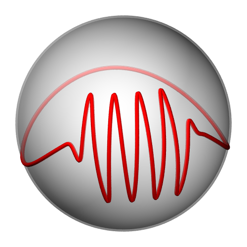
Figure 1: Without a lower bound on the thickness there is no longest curve on $\mbox{\smallthickmath S}^{2}$. Inserting more and more oscillations into a given curve its length can be made arbitrarily large.

1 The problem

What is the longest curve on the unit sphere? The most probable answer of any mathematically inclined person to this naïve question is: There is no such thing, since any spherical curve of finite length can be made arbitrarily long by replacing parts of it by more and more “wavy” arcs; see Figure 1. Rephrasing the initial query as “what is the longest rope on the unit sphere?” makes a big difference. A rope in contrast to a mathematical curve forms a solid body with positive thickness, so that now this question addresses a packing problem with obvious parallels in everyday life. Is there an optimal way of winding electrical cable onto the reel? Similarly, and economically quite relevant, can one maximize the volume of yarn wound onto a given bobbin [13], or how should one store long textile fibre band most efficiently to save storage space [12]?

Common to all these packing problems, in contrast to the classic Kepler problem of optimal sphere packing [2], [9], is that long and slender deformable objects are to be placed into a fixed volume or onto a given surface. Nature displays fascinating packing strategies on various scales. Extremely long strands of viral DNA are packed very efficiently into the tiny phage head of bacteriophages [3], and chromatin fibres are folded and organized in various aggregates within the chromatid [14].

To model a rope as a mathematical curve $\gamma$ with positive thickness we follow the approach of Gonzalez and Maddocks [7] who considered all triples of distinct curve points $x,y,z\in\gamma$, and their respective circumcircle radius $R(x,y,z)$. The smallest of these radii determines the curve’s thickness

$$\triangle[\gamma]:=\inf_{x\not=y\not=z\not=x\atop x,y,z\in\gamma}R(x,y,z).$$ (1.1)

A positive lower bound on this quantity controls local curvature but also prevents the curve from self-intersections; see Figure 2.

Figure 2: A positive thickness imposes a lower bound both on radius of curvature (left) as well as on global self-distance (right). The tubular neighbourhood around the curve does not self-intersect.

In fact, it equips the curve with a tubular neighbourhood of uniform radius $\triangle[\gamma]$ without self-penetration. It can be shown that positive thickness characterizes the set of embedded curves with bounded curvature [8, Lemmata 2 & 3], [15, Theorem 1], and we therefore tacitly assume from now on that our curves are simple, have positive length, and are continuously differentiable.

With this mathematical concept of thickness at our disposal we can reformulate the original question of finding the longest ropes on the unit sphere as a variational problem, where we first focus on closed loops.

Problem (P).

For a given constant $\Theta>0$ find the longest closed curve $\gamma:\mbox{\thickmath S}^{1}\cong\mbox{\thickmath R}/(2\pi\mbox{\thickmath Z})\to\mbox{\thickmath S}^{2}:=\{x\in\mbox{\thickmath R}^{3}:|x|=1\}$ with prescribed minimal thickness $\Theta$, i.e., with $\triangle[\gamma]\geq\Theta.$

Before discussing the solvability of this maximization problem for various thickness values we would like to point out that every loop $\gamma\subset\mbox{\thickmath R}^{3}$ of positive thickness enjoys a strong geometric property, the presence of forbidden balls: Any open ball $B_{\Theta}\subset\mbox{\thickmath R}^{3}$ of radius $\Theta\leq\triangle[\gamma]$ whose boundary $\partial B_{\Theta}$ touches the curve $\gamma$ tangentially in a point $p\in\gamma$, is not penetrated by the curve, that is $B_{\Theta}\cap\gamma=\emptyset.$ In fact, otherwise there were a point $q\in B_{\Theta}\cap\gamma$, and the plane spanned by the segment $q-p$ and the tangent vector of $\gamma$ at $p$ would intersect $B_{\Theta}$ in a planar disk of radius at most $\Theta.$ This disk would contain the strictly smaller circle through $q$ and $p$ that is tangent to the disk’s boundary in $p$. Approximating this circle by the circumcircles of the point triples $q,p,p_{i}$ for some sequence $\{p_{i}\}$ of curve points converging to $p$ as $i$ tends to infinity, yields a contradiction via $\triangle[\gamma]\leq R(p,q,p_{i})<\Theta$ for sufficiently large $i$.

A direct consequence of the presence of forbidden balls is that Problem (P) is not solvable at all if the prescribed thickness is strictly greater than $1$, there are simply no spherical curves whose thickness exceeds the value $1$. Indeed, for any point $p$ on a spherical curve $\gamma$ with thickness $\triangle[\gamma]>1$ there exists an open ball of radius $\triangle[\gamma]$ touching the unit sphere (and therefore $\gamma$ as well) in $p$ and containing all of the unit sphere but $p$. However, this ball is forbidden, hence contains no curve point so that $p$ is the only curve point on $\mbox{\thickmath S}^{2}.$ This settles Problem (P) for $\Theta>1.$

If we intersect the union of all forbidden touching balls $B_{\Theta}$, $\Theta\leq\triangle[\gamma]$ for a loop $\gamma\subset\mbox{\thickmath S}^{2}$, with the unit sphere, we easily deduce (see Figure 3) that every curve point of a spherical curve carries a pair of

Forbidden Geodesic Balls (FGB).

A closed spherical curve $\gamma:\mbox{\thickmath S}^{1}\to\mbox{\thickmath S}^{2}$ with (spatial) thickness $\triangle[\gamma]\geq\Theta>0$ does not intersect any open geodesic ball $\mathscr{B}_{\vartheta}(\xi):=\{\eta\in\mbox{\thickmath S}^{2}:{{\rm dist}_{\mbox{\smallthickmath S}^{2}}}(\eta,\xi)<\vartheta=\arcsin\Theta\}$ on $\mbox{\thickmath S}^{2}$ whose boundary $\partial\mathscr{B}_{\vartheta}(\xi)$ is tangent to $\gamma$ in at least one curve point. Here ${{\rm dist}_{\mbox{\smallthickmath S}^{2}}}(\cdot,\cdot)$ denotes the intrinsic distance on $\mbox{\thickmath S}^{2}$.

One can imagine a bow tie consisting of two open geodesic balls of spherical radius $\vartheta$ attached to the curve at their common boundary point. This bow tie can be moved freely along the curve without ever hitting any part of the curve.

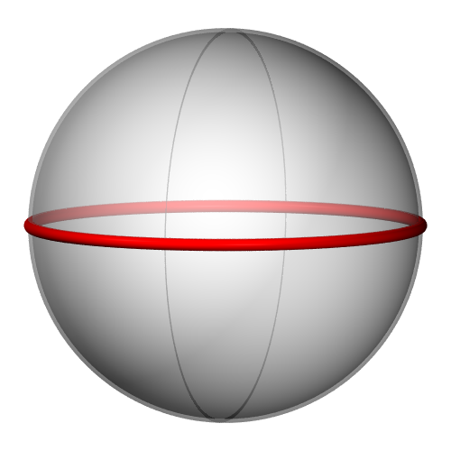
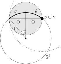
Figure 3: Left: A great-circle is the thickest curve on $\mbox{\smallthickmath S}^{2}$. Right: The unit sphere cut along a normal plane that is orthogonal to $\gamma$ at the point $p\in\gamma$. The grey spatial forbidden ball rotated along the dashed circle generates a forbidden geodesic ball of radius $\vartheta=\arcsin\Theta$ on $\mbox{\thickmath S}^{2}$.

The full strength of Property (FGB) is frequently used later on to completely classify infinitely many explicit solutions of Problem (P). For the moment it helps us to quickly solve that problem for $\Theta=1$. Take any point $p$ on an arbitrary spherical curve $\gamma$ with thickness $1$. The two forbidden open geodesic balls of spherical radius $\vartheta=\arcsin 1=\frac{\pi}{2}$ touching $\gamma$ in $p$ are two complementary hemispheres $\mbox{\thickmath S}^{+},\mbox{\thickmath S}^{-}$ that – according to (FGB) – do not intersect $\gamma.$ Hence $\gamma$ must be the equator as the only closed curve contained in the complement $\mbox{\thickmath S}^{2}\setminus(\mbox{\thickmath S}^{+}\cup\mbox{\thickmath S}^{-}).$ Thus the equator is the only spherical curve with thickness $1$ and hence – up to congruence – the unique solution to Problem (P) for $\Theta=1.$

But what about other thickness values $\Theta\in(0,1)$, is the variational problem (P) solvable at all? The answer is yes, and once one has analyzed the continuity properties of the constraint $\triangle[\gamma]\geq\Theta$, this can be proven with a direct method in the calculus of variations. The necessary arguments for this (and for the constructions and classification results in Sections 2 and 3) are carried out in full detail in [5]. Related existence results for thick elastic rods and ideal knots can be found in [8], [1], [6], [4].

Theorem 1.1 (Existence [5, Theorem 1.1]).

For each prescribed minimal thickness $\Theta\in(0,1]$ Problem (P) possesses (at least) one solution $\gamma_{\Theta}$. In addition, every such solution attains the minimal thickness, i.e., $\triangle[\gamma_{\Theta}]=\Theta.$

2 Infinitely many explicit solutions.

Knowing that solutions exist does not necessarily mean that we know their actual shape, unless $\Theta=1$ where we have identified the equator as the only solution. For general variational problems it is mostly impossible to extract explicit information about the shape of solutions, even uniqueness is usually a challenging issue. Here, however, the situation is different, and this has to do with the fact that every spherical curve $\gamma$ with positive thickness $\triangle[\gamma]=\Theta$ carries an open tubular neighbourhood

$$\mathscr{T}_{\vartheta}(\gamma):=\{\xi\in\mbox{\thickmath S}^{2}:{{\rm dist}_{\mbox{\smallthickmath S}^{2}}}(\gamma,\xi)<\vartheta=\arcsin\Theta\},$$

which equals the union of subarcs of great circles of uniform length $2\vartheta$ on the sphere. Each of these great-arcs is centered at a curve point $p\in\gamma$, and is orthogonal to the respective tangent vector of $\gamma$ at $p$. If two such great-arcs centered at different points $p,q\in\gamma$ had a common point, then $p$ would be contained in one of the forbidden geodesic balls touching $\gamma$ at $q$, which is excluded by Property (FGB). Therefore this union $\mathscr{T}_{\vartheta}(\gamma)$ of great-arcs is disjoint, and we conclude that a curve with (spatial) thickness $\triangle[\gamma]=\Theta$ has the larger spherical thickness $\vartheta=\arcsin\Theta>\Theta$.

It has been shown more than 70 years ago by Hotelling [10] and in more generality by Weyl [17] that the volume of such a uniform tubular neighbourhood is proportional to the length $\mathscr{L}$ of its centerline. Adapted to the present situation of thick curves on the unit sphere this classic theorem reads as

$${\rm area}(\mathscr{T}_{\vartheta}(\gamma))=2\sin\vartheta\cdot\mathscr{L}(\gamma)$$

for any curve $\gamma\subset\mbox{\thickmath S}^{2}$ with (spatial) thickness $\triangle[\gamma]\geq\Theta=\sin\vartheta.$ Consequently, any curve $\gamma\subset\mbox{\thickmath S}^{2}$ with thickness $\triangle[\gamma]\geq\Theta$ whose spherical tubular neighbourhood $\mathscr{T}_{\vartheta}(\gamma)$ covers all of $\mbox{\thickmath S}^{2}$, i.e., with

$${\rm area}(\mathscr{T}_{\vartheta}(\gamma))=4\pi={\rm area}(\mbox{\thickmath S}^{2}),$$ (2.2)

has maximal length among all spherical curves with prescribed minimal thickness $\Theta.$ In other words, sphere-filling thick curves provide solutions to Problem (P).

Are there any thickness values $\Theta\in(0,1)$ such that we find sphere-filling curves of that minimal thickness, i.e., curves $\gamma\subset\mbox{\thickmath S}^{2}$ with $\triangle[\gamma]\geq\Theta$ such that for $\vartheta=\arcsin\Theta$ we have Relation (2.2)?

If we relax for a moment our assumption that we search for one connected closed curve then we easily find sphere-filling ensembles of curves. For $\Theta_{n}:=\sin(\pi/2n)=:\sin\vartheta_{n}$, $n\in\mbox{\thickmath N}$, the stack of latitudinal circles $C_{i}$ with ${\rm dist}_{\mbox{\smallthickmath S}^{2}}(C_{0},\textnormal{north pole})=\vartheta_{n}$ and mutual distance ${\rm dist}_{\mbox{\smallthickmath S}^{2}}(C_{i},C_{i-1})=2\vartheta_{n}$ for $i=1,\ldots,n-1,$ forms a set of $n$ spherical curves each with spherical thickness $\vartheta_{n}=\pi/2n$. Their mutually disjoint spherical tubular neighbourhoods completely cover the sphere:

$${\rm area}\left[\bigcup_{i=0}^{n-1}\mathscr{T}_{\vartheta_{n}}(C_{i})\right]=4\pi.$$

This collection of latitudinal circles can now be used to construct one closed sphere-filling curve. Let us explain in detail how, for the case $n=4$. We cut the sphere with the $4$ latitudinal circles along a longitudinal into an eastern hemisphere $\mbox{\thickmath S}^{e}$ and a western hemisphere $\mbox{\thickmath S}^{w}$. Each hemisphere contains now a stack of $4$ latitudinal semicircles. Keeping the western hemisphere $\mbox{\thickmath S}^{w}$ fixed we rotate the eastern hemisphere $\mbox{\thickmath S}^{e}$ by an angle of $2\vartheta_{4}=\pi/4$ such that all the endpoints of the now turned semicircles on $\mbox{\thickmath S}^{e}$ meet endpoints of the semicircles on $\mbox{\thickmath S}^{w}$; see Figure 4.

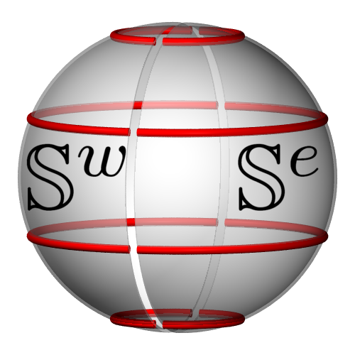
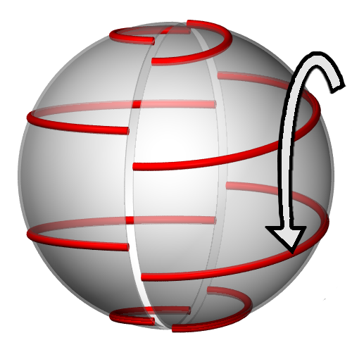
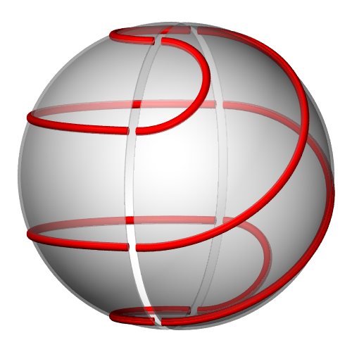
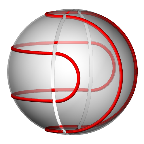
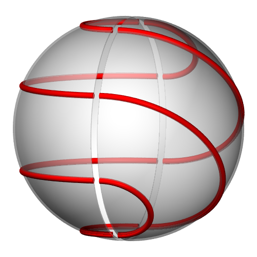
Figure 4: The construction of solutions for $n=4$. The third and the fifth image depict the sphere-filling curves for turning angles $2\vartheta_{4}$ and $6\vartheta_{4}$. The fourth image, in contrast, contains a disconnected sphere-filling ensemble with two components.

This modified collection of semicircles still has spherical thickness $\vartheta_{4}=\pi/8$ and is sphere-filling, since in the construction the sphere-filling stack of the original latitudinal circles was only cut orthogonally and reunited along one longitudinal, which does not change the thickness and sphere-filling property of the ensemble. We also observe that this new ensemble, which resembles to some extent the seamlines on a tennis ball, forms one closed curve, hence solves our problem – at least for this particular given spatial thickness $\Theta_{4}=\sin\vartheta_{4}=\sin(\pi/8).$ Are there other solutions for $n=4$? Why not continue rotating the eastern hemisphere $\mbox{\thickmath S}^{e}$ against the fixed hemisphere $\mbox{\thickmath S}^{w}$ to obtain more solutions? It turns out that a total rotation by $4\vartheta_{4}=\pi/2$ yields two connected components, which is not what we are looking for. But turning $\mbox{\thickmath S}^{e}$ by an angle of $6\vartheta_{4}=3\pi/4$ leads to another solution: a new single closed loop not congruent to the first one; see Figure 4.

One can show that this procedure works well for arbitrary $n\in\mbox{\thickmath N}$, and with a little elementary algebra we can determine the exact number of solutions:

Theorem 2.1 (Explicit solutions).

For each $n\in\mbox{\thickmath N}$ and each $k\in\{0,\ldots,n-1\}$ whose greatest common divisor with $n$ equals $1$, the construction described above starting with $n$ latitudinal circles $C_{0},\ldots,C_{n-1}$ with spherical distance

$${\rm dist}_{\mbox{\smallthickmath S}^{2}}(C_{0},\textnormal{north pole\,})=\vartheta_{n}=\frac{\pi}{2n},\quad{\rm dist}_{\mbox{\smallthickmath S}^{2}}(C_{i},C_{i-1})=2\vartheta_{n},\quad i=1,\ldots,n-1,$$

and rotating the eastern hemisphere against the fixed western hemisphere by an angle of $2k\vartheta_{n}$, leads to $\varphi(n)$ explicit piecewise circular solutions of the variational problem (P) for prescribed minimal thickness $\Theta_{n}=\sin\vartheta_{n}$.

Here, $\varphi$ denotes the Eulerian totient function from number theory: $\varphi(n)$ gives the number of integers $0\leq k<n$ so that the greatest common divisor of $k$ and $n$ equals $1$. In our example above, $n=4$, we indeed found $\varphi(4)=2$ explicit solutions by rotating the eastern hemisphere by the amount of $2k\vartheta_{4}$ for $k=1$ and for $k=3.$

Figure 5 depicts such sphere-filling closed curves for various $n$, and one notices a striking resemblance with certain so-called Turing patterns observed and analyzed in chemistry and biology as characteristic concentration distributions of different substances; see, e.g., [16]. In that context, the patterns are caused by diffusion-driven instabilities; here in contrast, the shape of solutions is a consequence of a simple variational principle.

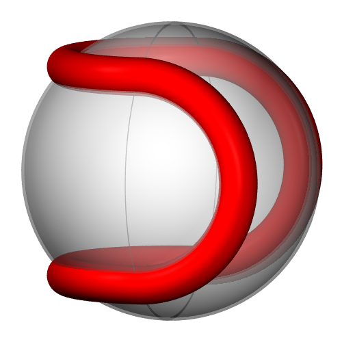
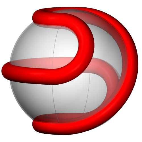
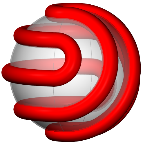
$n=2,k=1$	$n=3,k=1$	$n=5,k=2$
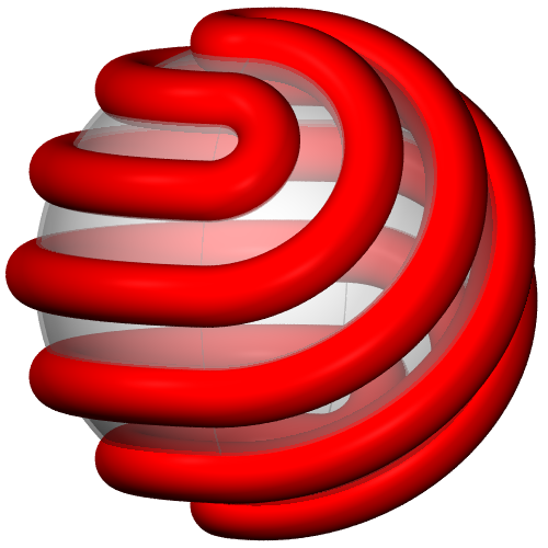
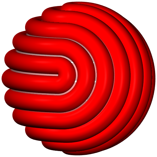
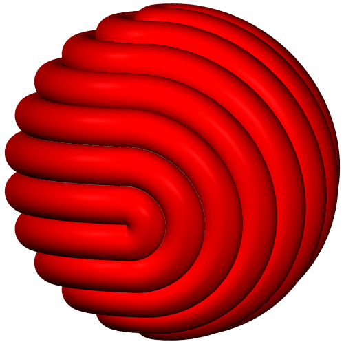
$n=7,k=2$	$n=11,k=5$	$n=12,k=7$

Figure 5: Various closed solutions of Problem (P). All curves are visualized as tubes of a fixed radius $\Theta=\pi/24$, which coincides with the actual spatial thickness $\triangle[\gamma]=\Theta_{n}$ only for the last curve with $n=12$. The remaining values of spatial thickness $\Theta_{n}$ for $n=1,\ldots,11,$ all exceed the tubes’ radii depicted in the image.

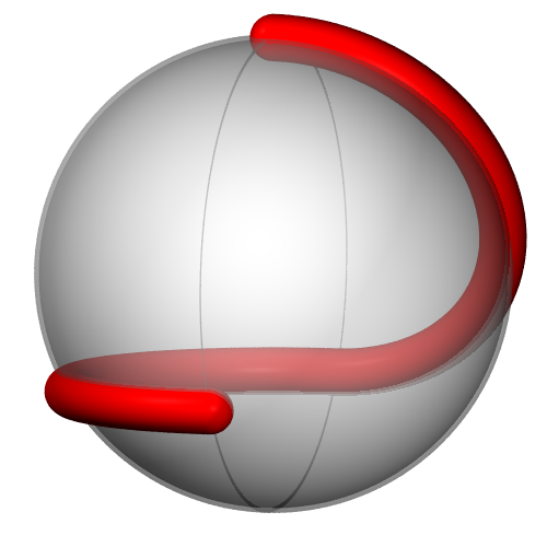
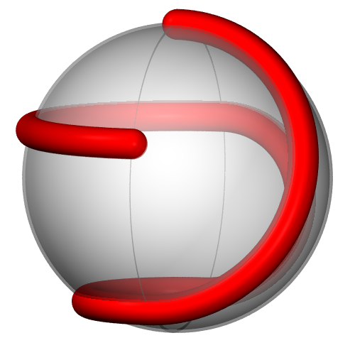
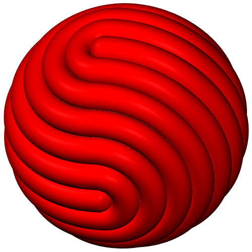
$n=3,k=1$	$n=5,k=1$	$n=25,k=6$
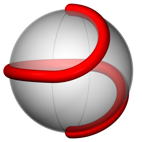
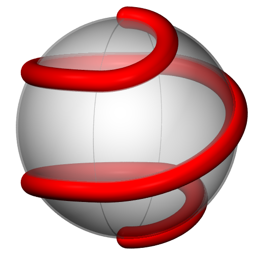
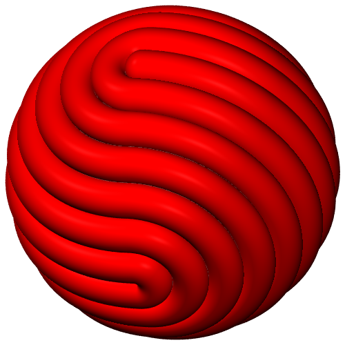
$n=4,k=0$	$n=6,k=0$	$n=26,k=0$

Figure 6: Various open solutions of Problem (P). Only the last ones in each row are depicted with full spatial thickness.

Similar constructions for thickness values $\Omega_{n}:=\sin(\pi/n),$ $n\in\mbox{\thickmath N}$, starting from an initial ensemble of semicircles together with one or two poles on $\mbox{\thickmath S}^{2}$, lead to two disjoint families of sphere-filling open curves distinguished by the relative position of the two endpoints on the sphere; see Figure 6. For all even $n\in\mbox{\thickmath N}$ the respective open sphere-filling curves have antipodal endpoints, which is not the case if $n$ is odd. Let us point out that these open curves occur in the different context of statistical physics, namely as two of three possible configurations of ordered phases of long elastic rods densely stuffed into spherical shells; see [11], in particular their figures 4a and 4c. Those studies aimed at explaining the possible nematic order of densely packed long DNA in viral capsids.

3 Classification of sphere-filling ropes

For each positive integer $n$ we have constructed explicitly longest closed ropes of thickness $\Theta_{n}=\sin(\pi/2n)$ on the unit sphere. Are there more? We know there are, for intermediate values $\Theta\not=\Theta_{n}$ by Theorem 1.1, but even if we stick to these specific countably many values $\Theta_{n}$ of given minimal thickness we might find more sphere-filling and thus length maximizing curves of considerably different shapes? The answer may be surprising, but, no, up to congruence our solutions are the only ones, and this “uniqueness” result is actually a consequence of a complete classification of sphere-filling thick curves:

Theorem 3.1 (Classification of sphere-filling loops).

If the spherical tubular neighbourhood $\mathscr{T}_{\vartheta}(\gamma),$ $\vartheta\in(0,\pi/2]$ of a closed spherical curve $\gamma\subset\mbox{\thickmath S}^{2}$ with thickness $\triangle[\gamma]\geq\Theta=\sin\vartheta$ satisfies

$${\rm area}(\mathscr{T}_{\vartheta}(\gamma))=4\pi={\rm area}(\mbox{\thickmath S}^{2}),$$

then there exist positive integers $n$, and $k\in\{0,\ldots,n-1\}$ with greatest common divisor equal to $1$, such that $\vartheta=\vartheta_{n}=\pi/(2n),$ $\triangle[\gamma]=\Theta_{n}=\sin\vartheta_{n},$ and such that $\gamma$ coincides – up to congruence – with one of the $\varphi(n)$ explicit solutions of Problem (P) exhibited in Theorem 2.1.

An analogous result holds also for open curves: any sphere-filling thick open curve must have spherical thickness $\omega_{n}=\arcsin\Omega_{n}=\pi/n$ for some $n\in\mbox{\thickmath N}$, and coincides with a member of one of the two explicitly constructed families of open spherical curves, depending on whether $n$ is even or odd. So, if one was given the (somewhat strange) task to produce a soccer ball of a given size by deforming a continuous piece of thick rope of suitable length into an airtight spherical hull, then only specific values of rope thickness are possible, and our theorem tells us how one should proceed. There is simply no other way!

Let us explain the main ideas of the proof of this classification result. The presence of forbidden geodesic balls (FGB) allows us to prove a fundamental touching principle for spherical curves $\gamma$ with positive thickness $\triangle[\gamma]$; see Part A below. This principle guarantees then that the number of possible local touching situations between the curve and geodesic balls with radius equal to $\triangle[\gamma]$ is very limited (Part B). The combination of these pieces of information leads to a geometric rigidity for sphere-filling curves reflected in two sorts of possible global patterns (Part C).

Figure 7: A curve $\gamma$ with spherical thickness $\vartheta$ that touches a circle of radius $\vartheta$ in two non-antipodal points $P$ and $Q$, joins them with a subarc of that circle. Otherwise one of the dotted circles would intersect $\gamma$ three times leading to a lower thickness.

A. The touching principle  addresses the situation when a spherical curve $\gamma$ with $\triangle[\gamma]\geq\Theta=\sin\vartheta$ touches the boundary $\partial\mathscr{B}_{\vartheta}(\xi_{0})$ of a geodesic ball $\mathscr{B}_{\vartheta}(\xi_{0})$ in $\mbox{\thickmath S}^{2}$ in at least two non-antipodal points $P,Q\in\partial\mathscr{B}_{\vartheta}(\xi_{0})$ with ${{\rm dist}_{\mbox{\smallthickmath S}^{2}}}(P,Q)=:2\vartheta_{1}<2\vartheta.$ In this situation the boundary of the strictly smaller geodesic ball $\mathscr{B}_{\vartheta_{1}}(\xi_{1})$ for which $P$ and $Q$ are antipodal, is intersected transversally by $\gamma$ in $P$ and $Q$, which means that the open geodesic ball $\mathscr{B}_{\vartheta_{1}}(\xi_{1})$ contains curve points; see Figure 7. On the other hand, $\partial\mathscr{B}_{\vartheta_{1}}(\xi_{1})$ contains no further curve point $T$ different from $P$ and $Q$, since this would imply for the corresponding (Euclidean) circumcircle

$$R(P,Q,T)\leq\sin\vartheta_{1}<\sin\vartheta=\Theta$$ (3.3)

contradicting our assumption $\triangle[\gamma]\geq\Theta$; recall Formula (1.1). Consequently, there is a whole subarc of $\gamma$ connecting $P$ and $Q$ contained in $\mathscr{B}_{\vartheta_{1}}(\xi_{1}),$ but not in the original larger ball $\mathscr{B}_{\vartheta}(\xi_{0})$ since this one is a forbidden ball according to (FGB). Where can we locate this arc within the set $\mathscr{B}_{\vartheta_{1}}(\xi_{1})\setminus\mathscr{B}_{\vartheta}(\xi_{0})$? Sweeping out the region $\mathscr{B}_{\vartheta_{1}}(\xi_{1})\setminus\overline{\mathscr{B}_{\vartheta}(\xi_{0})}$ with intermediate geodesic circles $\partial\mathscr{B}_{\vartheta_{s}}(\xi_{s})$ with center $\xi_{s}$ on the great arc connecting $\xi_{0}$ and $\xi_{1}$, and containing $P$ and $Q$ for each $s\in[0,1]$ (so that $\vartheta_{s}=|P-\xi_{s}|$, $\vartheta_{0}:=\vartheta$) we use the same argument as the one that led to (3.3) to show that there are no curve points in $\mathscr{B}_{\vartheta_{1}}(\xi_{1})\setminus\overline{\mathscr{B}_{\vartheta}(\xi_{0})}.$ Thus we have proven the

Touching Principle (TP).

A closed spherical curve $\gamma:\mbox{\thickmath S}^{1}\to\mbox{\thickmath S}^{2}$ with (spatial) thickness $\triangle[\gamma]\geq\Theta=\sin\vartheta$ that touches tangentially a geodesic circle $\partial\mathscr{B}_{\vartheta}\subset\mbox{\thickmath S}^{2}$ of spherical radius $\vartheta$ in two non-antipodal points $P$ and $Q$, contains the shorter circular subarc of $\partial\mathscr{B}_{\vartheta}$ connecting $P$ and $Q$.

We benefit from the touching principle since it allows us to characterize sphere-filling curves of thickness $\Theta=\triangle[\gamma]=\sin\vartheta$ in terms of their local behaviour when touching geodesic balls of spherical radius $\vartheta$: For any open geodesic ball $\mathscr{B}_{\vartheta}$ disjoint from $\gamma$ – and there are plenty of those, e.g., all forbidden balls by (FGB) – then one of the following three touching situations is guaranteed for the intersection $\mathscr{S}:=\partial\mathscr{B}_{\vartheta}\cap\gamma$:

B. Possible local touching situations.

1. $\gamma$ touches $\partial\mathscr{B}_{\vartheta}$ in exactly two antipodal points, i.e., $\mathscr{S}=\{P,Q\}$ with ${{\rm dist}_{\mbox{\smallthickmath S}^{2}}}(P,Q)=2\vartheta$, or

2. the intersection $\mathscr{S}$ is a relatively closed semicircle of spherical radius $\vartheta$, or

3. this intersection $\mathscr{S}$ equals the full geodesic circle $\partial\mathscr{B}_{\vartheta}.$

To see this we notice first that for a sphere-filling curve the relatively closed intersection $\mathscr{S}$ is nonempty, since otherwise a slightly larger ball $\mathscr{B}_{\vartheta+\epsilon}$ for some small positive $\epsilon$ would not contain any curve point, which leads to $\mathscr{B}_{\epsilon}\cap\mathscr{T}_{\vartheta}(\gamma)=\emptyset,$ and hence $4\pi={\rm area}(\mathscr{T}_{\vartheta}(\gamma))\leq{\rm area}(\mbox{\thickmath S}^{2}\setminus\mathscr{B}_{\epsilon})<4\pi$ contradicting (2.2).

Similarly, one can rule out that the set $\mathscr{S}$ is contained in a relatively open semicircle on $\partial\mathscr{B}_{\vartheta}$, since then two extremal points $\eta,\zeta\in\mathscr{S}$ realizing the diameter of $\mathscr{S}$ would have spherical distance ${{\rm dist}_{\mbox{\smallthickmath S}^{2}}}(\eta,\zeta)<2\vartheta.$ This is one of the frequent occasions that the touching principle (TP) comes into play. It implies that the whole circular subarc of $\partial\mathscr{B}_{\vartheta}$ connecting $\eta$ and $\zeta$, is contained in $\mathscr{S}$ and therefore equals $\mathscr{S}$ in this situation. But the fact that $\gamma$ lifts off the geodesic circle $\partial\mathscr{B}_{\vartheta}$ at $\eta$ and $\zeta$ before completing a full semicircle allows us to move the closed ball $\overline{\mathscr{B}_{\vartheta}}$ slightly “away” from $\mathscr{S}$, that is, in the direction orthogonal to and away from the geodesic arc connecting $\eta$ and $\zeta.$ This way we obtain a slightly shifted closed ball of the same radius without any contact to $\gamma$, a situation that we have ruled out above. Therefore, $\mathscr{S}$ is not contained in any relatively open semicircle on $\partial\mathscr{B}_{\vartheta}.$

If $\mathscr{S}$ is contained in a relatively closed semicircle we may assume that it contains apart from the antipodal endpoints of that semicircle also at least one third point, otherwise we were in Situation (a) and could stop here. Therefore, by virtue of the touching principle (TP) $\mathscr{S}$ coincides completely with that closed semicircle, which is Option (b). If, however, $\mathscr{S}$ is not contained in any semicircle we can simply look at one point $q\in\mathscr{S}$ and its antipodal point $q^{\prime}\in\partial\mathscr{B}_{\vartheta}$. If $q^{\prime}$ happens to be also in $\gamma$, then both semicircles connecting $q$ and $q^{\prime}$ would contain further curve points and therefore $\mathscr{S}=\partial\mathscr{B}$ again by the touching principle, and we end up with Option (c).

If $q^{\prime}\not\in\mathscr{S}$, then the largest open subarc $\alpha$ of $\partial\mathscr{B}_{\vartheta}$ containing $q^{\prime}$ but no point of $\gamma$ must be shorter than $\pi$ unless $\mathscr{S}$ is contained in a semicircle, a situation we brought to a close before. Applying the touching principle to the two endpoints of $\alpha$ we find in fact that $q^{\prime}$ lies on the subarc of $\gamma$ connecting these endpoints on $\partial\mathscr{B}_{\vartheta},$, which exhausts the last possible situation to verify that our list of situations (a)–(c) is complete.

We are going to use the local structure established in Parts A and B to prove geometric rigidity of sphere-filling curves $\gamma$ with positive spatial thickness $\Theta=\sin\vartheta.$

C. Global patterns of sphere-filling curves.

(C1).

If $\gamma\subset\mbox{\thickmath S}^{2}$ intersects a normal plane $E$ orthogonally in $k$ distinct points whose mutual spherical distance equals $2\vartheta$, then $k$ is even and $\gamma$ contains a semicircle of spherical radius $\vartheta$ in each of the two hemispheres bounded by $E\cap\mbox{\thickmath S}^{2}$.

(C2).

If $\gamma$ contains one latitudinal semicircle $S\subset\partial\mathscr{B}_{\vartheta}$, then $\vartheta=\pi/2n$ for some $n\in\mbox{\thickmath N}$ and the portion of $\gamma$ in the corresponding hemisphere consists of the whole stack of $n$ latitudinal semicircles (including $S$) with mutual spherical distance $\vartheta.$

Before providing the proofs for these rigidity results let us explain how we can combine these to establish the

Proof of Theorem 3.1.  The goal is to show the existence of a latitudinal semicircle of spherical radius $\vartheta$ contained in $\gamma$ in order to apply the global pattern (C2), which then assures that $\gamma$ consists of a stack of latitudinal semicircles with mutual spherical distance $\vartheta$ in one hemisphere, say in $\mbox{\thickmath S}^{w}$. This behaviour in $\mbox{\thickmath S}^{w}$ leads to the characteristic intersection point pattern in the longitudinal circle $\partial\mbox{\thickmath S}^{w}$ needed in order to apply (C1), which in turn guarantees the existence of a semicircle of radius $\vartheta$ on $\mbox{\thickmath S}^{e}$ whose endpoints meet $\partial\mbox{\thickmath S}^{e}$ orthogonally. Again property (C2) leads to a whole stack of $n$ equidistant semicircles now on $\mbox{\thickmath S}^{e}$. Our construction described in Section 2 finally reveals the only possible loops made of two such stacks of equidistant latitudinal semicircles meeting $\partial\mbox{\thickmath S}^{e}=\partial\mbox{\thickmath S}^{w}$ orthogonally, which completes the proof of the classification theorem. The logic of proof resembles a ride on the merry-go-round; (C1) produces the semicircle on $\mbox{\thickmath S}^{w}$ necessary to use (C2) to obtain the stack of semicircles on $\mbox{\thickmath S}^{w}$, which itself generates the point pattern needed to apply (C1) on $\mbox{\thickmath S}^{e}$ and finish the task via (C2) on $\mbox{\thickmath S}^{e}.$ The only problem is: how do we enter the merry-go-round? We have to show that one portion of $\gamma$ is a semicircle of spherical radius $\vartheta$ without assuming the intersection point pattern needed in (C1).

Let $k$ be the integer such that $(k-1)\vartheta<\pi\leq k\vartheta.$ For a fixed point $p\in\gamma$ we walk along a unit speed geodesic ray $\eta_{p}$ emanating from $p$ in a direction orthogonal to $\gamma$ at $p$ in search of such a semicircle. The geodesic ball $\mathscr{B}_{\vartheta}(\eta_{p}(\vartheta))$ is a forbidden ball by means of (FGB), i.e., $\gamma\cap\mathscr{B}_{\vartheta}(\eta_{p}(\vartheta))=\emptyset,$ where $\eta_{p}(\vartheta)$ denotes the point reached on the geodesic ray after a spherical distance $\vartheta.$ According to the possible local touching situations we find the desired semicircle on $\partial\mathscr{B}_{\vartheta}(\eta_{p}(\vartheta)\cap\gamma$ (Option (b) or (c) in B), unless the antipodal point $\eta_{p}(2\vartheta)$ is contained in $\gamma.$ In that case we continue along the same geodesic ray passing through $\eta_{p}(2\vartheta)$ orthogonally to $\gamma$, until we either find a closed semicircle on one of the geodesic circles $\partial\mathscr{B}_{\vartheta}((2i-1)\vartheta))$, $i=1,\ldots,k,$ or $\vartheta=\pi/k,$ and all “antipodal points” $\eta_{p}(2i\vartheta)$ are contained in $\gamma$, so that $\eta_{p}(2k\vartheta)=p.$ In other words, either we have found the desired semicircle during the walk along $\eta_{p}$, or we have walked once around the whole longitudinal circle traced out by $\eta_{p}$ generating $k$ equidistant points where $\gamma$ intersects $\eta_{p}$ orthogonally. But this is exactly what is needed to apply (C1) to finally establish the existence of the semicircle we are looking for.

One final comment on why this exact quantization takes place, i.e., why we find $\vartheta=\pi/k$ so that the walk along $\eta_{p}$ pinpointing the centers $\eta_{p}((2i-1)\vartheta)$ of geodesic balls on the way, actually leads exactly back to the starting point $p=\eta_{p}(2\pi).$ The successive localization of forbidden balls according to (FGB) and the possible local touching situations yield the fact that all open geodesic balls $\mathscr{B}_{\vartheta}(\eta_{p}((2i-1)\vartheta)$ for $i=1,\ldots,k$, are disjoint from $\gamma.$ If, for instance, the walk had stopped too late since the step size $\vartheta$ was too large, $k\vartheta>\pi$, then ${{\rm dist}_{\mbox{\smallthickmath S}^{2}}}(p,\eta_{p}(2k-1)\vartheta)=2\pi-(2k-1)\vartheta<\vartheta$, that is, $p\in\mathscr{B}_{\vartheta}(\eta_{p}(2k-1)\vartheta)\cap\gamma$, a contradiction. A similar argument works if we had stopped our walk too early.∎

Let us establish the global patterns (C1) and (C2) in more detail since they served as the core tools in the proof of our classification theorem.

We start with the proof of (C1). Here it suffices to focus on one of the two hemispheres $\mbox{\thickmath S}^{w}$ and $\mbox{\thickmath S}^{e}$ determined by $E$, say on $\mbox{\thickmath S}^{w}$. Since $\gamma$ is simple and closed the curve can leave $\mbox{\thickmath S}^{w}$ merely as often as it enters $\mbox{\thickmath S}^{w}$, which immediately gives $k=2n$ for some $n\in\mbox{\thickmath N}$. Moreover, $\mbox{\thickmath S}^{w}$ is homeomorphic to a flat disk so that we can find nearest neighbouring exit and entrance points $p,q\in E\cap\gamma$ with minimal spherical distance ${{\rm dist}_{\mbox{\smallthickmath S}^{2}}}(p,q)=2\vartheta$ such that the closed subarc $\beta\subset\mbox{\thickmath S}^{w}\cap\gamma$ connecting $p$ and $q$ satisfies $E\cap\beta=\{p,q\}.$ We will show that $\beta$ contains the desired semicircle of spherical radius $\vartheta$. Since $\gamma$ intersects $E$ orthogonally we infer from (FGB) that the open geodesic ball $\mathscr{B}\equiv\mathscr{B}_{\vartheta}$ containing $p,q\in\partial\mathscr{B}$ as antipodal boundary points, is disjoint from $\gamma$. If there were a third point $b\in\beta\cap\partial\mathscr{B}$ distinct from $p$ and $q$, then – according to the touching principle (TP) – the whole semicircle on $\partial\mathscr{B}$ with endpoints $p$ and $q$ would be contained in $\gamma$, and we were done. Else we trace the open spherical region $\mathscr{R}$ bounded by $\beta\cup(\mbox{\thickmath S}^{e}\cap\partial\mathscr{B})$ with geodesic rays $\eta_{b}$ emanating from arbitrary points $b\in\beta$ orthogonally into the region $\mathscr{R}.$ Notice that $\mathscr{R}$ is disjoint from $\gamma$, and that $\eta_{p}(2\vartheta)=q$ and $\eta_{q}(2\vartheta)=p$ where the argument of $\eta$ indicates how long one has to travel along the geodesic ray to reach the destination point. In addition, the forbidden ball property (FGB) implies $\gamma\cap\mathscr{B}_{\vartheta}(\eta_{b}(\vartheta))=\emptyset$ and therefore $\mathscr{B}_{\vartheta}(\eta_{b}(\vartheta))\subset\mathscr{R}$ for all points $b\in\beta;$ see Figure 8.

Figure 8: Towards the proof of (C1). Geodesic rays $\eta_{b}$ emanating from points $b$ on the subarc $\beta\subset\gamma\cap\mbox{\smallthickmath S}^{e}$ to trace the enclosed spherical region $\mathscr{R}$. The depicted antipodal touching (3.4) is excluded to hold throughout $\beta$ by virtue of Brouwer’s fixed point theorem.

According to Part B either

$$\partial\mathscr{B}_{\vartheta}(\eta_{b}(\vartheta))\cap\gamma=\{b,\eta_{b}(2\vartheta))\quad\,\,\,\text{for all }\,\,b\in\beta,$$ (3.4)

(the antipodal situation (a)), or $\gamma$ contains a semicircle $S_{b}=\partial\mathscr{B}_{\vartheta}(\eta_{b}(\vartheta))\cap\gamma$ containing itself the point $b$ for some $b\in\beta.$ This semicircle lies completely in the western hemisphere $\mbox{\thickmath S}^{w}$, which concludes the proof of (C1). To see the latter assume contrariwise that there exists a point $z$ on $\mbox{\thickmath S}^{e}\cap S_{b}\setminus E$. Then by connectivity also $p$ or $q$ would lie on the semicircle $S_{b}$, too, which immediately implies that $S_{b}$ and hence also $b\in\partial\mathscr{B}\cap\beta$ lies on the original geodesic circle $\partial\mathscr{B}$, a situation that we had excluded already.

It remains to exclude the antipodal touching (3.4) throughout the subarc $\beta\subset\gamma\cap\mbox{\thickmath S}^{w}$. We use Brouwer’s fixed point theorem for the continuous map $f:\beta\to\mbox{\thickmath S}^{2}$ defined by $f(b):=\eta_{b}(2\vartheta)$, which actually maps $\beta$ into $\beta$. Relation (3.4) in fact guarantees that $f(b)\in\gamma\setminus\mathscr{B}$ hence $f(b)$ is either contained in $\mbox{\thickmath S}^{w}\cap\overline{\mathscr{R}}\cap\gamma=\beta$ in which case we are done, or $f(b)$ lies in $\partial\mathscr{B}\cap\mbox{\thickmath S}^{e}\cap\gamma.$ But then the antipodal partner $b$ of $f(b)$ would also lie on $\partial\mathscr{B}$, which was excluded earlier. Consequently, Brouwer’s theorem is applicable and leads to a fixed point $b^{*}=f(b^{*})=\eta_{b^{*}}(2\vartheta)$, which implies $2\vartheta=2\pi$ because $\eta_{b^{*}}$ parametrizes a unit speed great circle on $\mbox{\thickmath S}^{2}$. But this contradicts our assumption that $\vartheta\in(0,\pi/2].$ ∎

The proof of (C2) can be sketched as follows. Let $n$ be the integer such that $\pi/(2n)\leq\vartheta<\pi/(2n-2).$ According to (FGB) one has a forbidden ball: $\gamma\cap\mathscr{B}_{\vartheta}=\emptyset$, and the idea is to start from the initial semicircle $S_{1}:=S\subset\partial\mathscr{B}_{\vartheta}$ and “scan” the remaining part $\mbox{\thickmath S}^{2}\setminus\overline{\mathscr{B}_{\vartheta}}$ with unit speed geodesic rays $\eta_{p}$ emanating from every point $p\in S_{1}$ orthogonally to $S_{1}$ into the open region $\mbox{\thickmath S}^{2}\setminus\overline{\mathscr{B}_{\vartheta}}$. Again by (FGB) we find $\mathscr{B}_{\vartheta}(\eta_{p}(\vartheta))\cap\gamma=\emptyset$ for each such starting point $p\in S_{1}$. All possible touching situations documented in Part B guarantee the existence of at least one second curve point $q$ on $\partial\mathscr{B}_{\vartheta}(\eta_{p}(\vartheta)),$ and we claim that $q$ must be antipodal to $p$, i.e., $q=\eta_{p}(2\vartheta)$. If not, then according to Options (b) or (c) in Part B, the points $p$ and $q$ are contained in a semicircle on $\partial\mathscr{B}_{\vartheta}(\eta_{p}(\vartheta))\cap\gamma.$ But this semicircle is hit by neighbouring geodesic “scanning” rays $\eta_{r}$ emanating from $r\in S_{1}$ for $r$ close to $p$, which would lead to a nonempty intersection of $\gamma$ with the neighbouring forbidden ball $\mathscr{B}_{\vartheta}(\eta_{r}(\vartheta))$ contradicting (FGB). Hence we have shown that only antipodal curve points can be generated by this procedure: $\partial\mathscr{B}_{\vartheta}(\eta_{p}(\vartheta))\cap\gamma=\{p,\eta_{p}(2\vartheta))$ for all $p\in S_{1}$, which produces a second semicircle $S_{2}:=\bigcup_{p\in S_{1}}\eta_{p}(2\vartheta)=\partial\mathscr{B}_{3\vartheta}$ contained in $\gamma$, with spherical distance $2\vartheta$ to the first semicircle $S_{1}$.

It is obvious how to continue this procedure – now starting the “scanning” rays from $S_{2}$ – to obtain a whole stack of semicircles $S_{i}=\partial\mathscr{B}_{(2i-1)\vartheta}$ for $i=1,\ldots,n.$ If this stack is too high because the spherical thickness is too large with respect to $n$, i.e., if $\pi/(2n-1)\leq\vartheta<\pi/(2n-2)$, then the stack would “spill over” onto the other hemisphere $\mbox{\thickmath S}^{e}$ producing a final semicircle $S_{n}$ contained in $\mbox{\thickmath S}^{e}\cap\gamma$ with spherical radius $(2n-1)\vartheta-\pi\in[0,\vartheta)$ that is too small: it contradicts the spherical thickness $\vartheta=\arcsin\triangle[\gamma]$ of $\gamma$ since its curvature is to large. If the stack is not high enough ($\pi/2n<\vartheta<\pi/(2n-1)$) then the last semicircle $S_{n}$ is still on the correct hemisphere $\mbox{\thickmath S}^{w}$ but has spherical radius $\pi-(2n-1)\vartheta\in(0,\vartheta)$, which is again to small for the thick curve $\gamma.$∎

4 Final Remark

For an infinite countable number of thickness values we have established a complete picture of the solution set for Problem (P) using the sphere-filling property to a large extent. The general existence theorem, Theorem 1.1, however, guarantees the existence of longest ropes on the unit sphere also for all intermediate thickness values $\Theta\not=\Theta_{n}$. What are their actual shapes? Theorem 3.1 ascertains that those solutions cannot be sphere-filling. In [5] we constructed a comparison curve that could serve as a promising candidate for prescribed minimal thickness $\Theta\in(\Theta_{2},\Theta_{1})$, but this question remains to be investigated, as well as the interesting connections to Turing patterns and the statistical behaviour of long elastic rods under spherical confinement mentioned in Sections 1 and 2. In addition, if one substitutes the unit sphere by other supporting manifolds such as the standard torus, then the issue of analyzing the shapes of optimally packed ropes is wide open.

References

- [1] Cantarella, J.; Kusner, R.B.; Sullivan, J.M. On the minimum ropelength of knots and links. Inv. math. 150 (2002), 257–286.
- [2] Conway, J.H.; Sloane, N.J.A. Sphere Packings, Lattices and Groups. Springer, New York 1988.
- [3] Earnshaw, W.C.; Harrison, S.C. DNA arrangement in isometric phage heads. Nature 268 (1977), 598–602.
- [4] Gerlach, H.; Maddocks, J.H. Existence of ideal knots in . in preparation
- [5] Gerlach, H.; von der Mosel, H. What are the longest ropes on the unit sphere? Preprint Nr. 32 Inst. f. Mathematik, RWTH Aachen University 2009.
- [6] Gonzalez, O.; de la Llave, R. Existence of Ideal Knots. J. Knot Theory Ramifications 12 (2003), 123–133.
- [7] Gonzalez, O.; Maddocks, J.H. Global Curvature, Thickness and the Ideal Shapes of Knots. Proc. Natl. Acad. Sci. USA 96 (1999), 4769–4773.
- [8] Gonzalez, O.; Maddocks, J.H.; Schuricht, F.; von der Mosel, H. Global curvature and self-contact of nonlinearly elastic curves and rods. Calc. Var. 14 (2002), 29–68.
- [9] Hales, T.C. Cannonballs and honeycombs. Notices AMS 47 (2000), 440–449.
- [10] Hotelling, H. Tubes and Spheres in -Spaces. Amer. J. Math. 61 (1939), 440–460.
- [11] Katzav, E.; Adda-Bedia, M.; Boudaoud, A. A statistical approach to close packing of elastic rods and to DNA packaging in viral capsids. Proceedings of the National Academy of Sciences, USA, 103 (2006), 18900–18904.
- [12] Kyosev, Y. Numerical analysis for sliver winding process with additional can motion. In: 5th International Conference Textile Science 2003 TEXSCI 2003, ISBN 80-7083-711-X, TU-Liberec, Czech Republic (2003), pp. 330-334.
- [13] Mayer, M.; Lenz, F. Method and apparatus for winding a yarn into a package. US Patent 6186435 (issued 2001).
- [14] Mullinger, A.M.; Johnson, R.T. Units of chromosome replication and packing. J. Cell Sci. 64 (1983), 179–193.
- [15] Schuricht, F.; von der Mosel, H. Global curvature for rectifiable loops. Math. Z. 243 (2003), 37–77.
- [16] Varea, C.; Aragon, J.L.; Barrio, R.A. Turing patterns on a sphere. Phys. Rev. E 60 (1999), 4588–4592.
- [17] Weyl, H. On the volume of tubes. Amer.J. Math. 61 (1939), 461–472.
- [18] Wiggs, C.C.; Taylor, C.J.C. Bead puzzle. US Patent D269629 (issued 1983).
Henryk Gerlach
IMB / LCVMM
Station 8
Faculté des Sciences de Base
EPFL Lausanne
CH-1015 Lausanne
SWITZERLAND
E-mail: henryk.gerlach@
epfl.ch
Heiko von der Mosel
Institut für Mathematik
RWTH Aachen University
Templergraben 55
D-52062 Aachen
GERMANY
E-mail: heiko@
instmath.rwth-aachen.de