Magnetic Response in Mesoscopic Hubbard Rings: A Mean Field Study

Abstract

The present work proposes an idea to remove the long standing controversy between the calculated and measured current amplitudes carried by a small conducting ring upon the application of an Aharonov-Bohm (AB) flux $\phi$. Within a mean field Hartree-Fock (HF) approximation we numerically calculate persistent current, Drude weight, low-field magnetic susceptibility and related issues. Our analysis may be inspiring for studying magnetic response in nano-scale loop geometries.

I Introduction

In mesoscopic range phase coherence of electronic states is of fundamental importance and the existence of dissipationless current in a mesoscopic conducting ring threaded by an Aharonov-Bohm (AB) flux $\phi$ is a spectacular consequence of quantum phase coherence. The existence of persistent current in mesoscopic rings has been addressed several years ago in the pioneering work of Büttiker, Imry and Landauer butt . Later, many excellent experiments levy ; chand ; jari ; deb have been done in different systems to reveal the phenomenon of persistent current. Though in literature many theoretical cheu1 ; cheu2 ; peeters1 ; peeters2 ; peeters3 ; mont ; alts ; von ; schm ; ambe ; bouz ; giam ; yu ; san1 ; san2 ; san3 ; san4 as well as experimental papers levy ; chand ; jari ; deb on persistent current are available, yet lot of controversies are still present between the theory and experiment, and the complete knowledge about it in this scale is not very well established even today. The unexpectedly large amplitudes of measured currents provide to the most important controversy. It has been proposed that the electron-electron (e-e) interactions contribute significantly to the average currents. An explanation based on the perturbative calculation in presence of interaction and disorder has been proposed and it seems to give a quantitative estimate closer to the experimental results, but still it is less than the measured currents by an order of magnitude, and the interaction parameter used in the theory is not well understood physically. Though an attempt has been made to explain the enhancement of current amplitude by some theoretical arguments but the sign of low-field currents cannot be predicted precisely and it is an important controversial issue between theoretical and experimental results.

Motivated with these open challenges in the present paper we address magnetic response in mesoscopic Hubbard rings threaded by AB flux $\phi$. We try to propose an idea to remove the unexpected discrepancy between the calculated and measured current amplitudes by incorporating the effect of second-neighbor hopping (SNH) in addition to the traditional nearest-neighbor hopping (NNH) integral in the tight-binding Hamiltonian. Using a generalized Hartree-Fock (HF) approximation kato ; kam ; sil , we numerically compute persistent current ($I$), Drude weight ($D$) and low-field magnetic susceptibility ($\chi$) as functions of AB flux $\phi$, total number of electrons $N_{e}$ and system size $N$. With this (HF) approach one can study magnetic response in a much larger system since here a many-body Hamiltonian is decoupled into two effective one-body Hamiltonians. One is associated with up spin electrons and other is related to down spin electrons. But the point is that, the results calculated using generalized HF mean-field theory may deviate from exact results with the reduction of

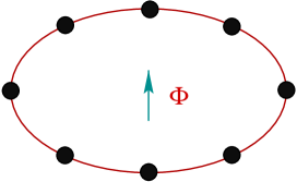
Figure 1: (Color online). Schematic view of a $1$D mesoscopic ring penetrated by a magnetic flux $\phi$. The filled black circles correspond to the positions of the atomic sites.

dimensionality. So we should take care about the mean-field calculation, specially, in one-dimensional systems. To trust our predictions, in the present work also we make a comparative study between the results obtained from mean-field theory and exactly diagonalizing the full many-body Hamiltonian. The later approach where a complete many-body Hamiltonian is diagonalized to get energy eigenvalues is not suitable to study magnetic response in larger systems since the size of the matrices increases very sharply with the total number of up and down spin electrons. Our results can be utilized to explore magnetic response in any interacting mesoscopic system.

We organize the paper as follows. Following a brief introduction (Section I), in Section II we describe the geometric model and generalized Hartree-Fock theory to study magnetic response in the model quantum system. Section III contains the numerical results, and finally, summary of our work will be available in Section IV.

II Model and theoretical formulation

We start by referring to Fig. 1, where a normal metal ring is threaded by a magnetic flux $\phi$. To describe the system we use a tight-binding framework. For a $N$-site ring, penetrated by a magnetic flux $\phi$ (measured in unit of the elementary flux quantum $\phi_{0}=ch/e$), the tight-binding Hamiltonian in Wannier basis looks in the form,

$$H_{R} = \sum_{i,\sigma}\epsilon_{i\sigma}c_{i\sigma}^{\dagger}c_{i\sigma}+\sum_{ij,\sigma}t\left[e^{i\theta}c_{i\sigma}^{\dagger}c_{j\sigma}+h.c.\right]+$$ (1)

$$\sum_{ik,\sigma}t_{1}\left[e^{i\theta_{1}}c_{i\sigma}^{\dagger}c_{k\sigma}+h.c.\right]+\sum_{i}Uc_{i\uparrow}^{\dagger}c_{i\uparrow}c_{i\downarrow}^{\dagger}c_{i\downarrow}$$

where, $\epsilon_{i\sigma}$ is the on-site energy of an electron at the site $i$ of spin $\sigma$ ($\uparrow,\downarrow$). The variable $t$ corresponds to the nearest-neighbor ($j=i\pm 1$) hopping strength, while $t_{1}$ gives the second-neighbor ($k=i\pm 2$) hopping integral. $\theta=2\pi\phi/N$ and $\theta_{1}=4\pi\phi/N$ are the phase factors associated with the hopping of an electron from one site to its neighboring site and next-neighboring site, respectively. $c_{i\sigma}^{\dagger}$ and $c_{i\sigma}$ are the creation and annihilation operators, respectively, of an electron at the site $i$ with spin $\sigma$. $U$ is the strength of on-site Hubbard interaction.

II.1 Decoupling of the interacting Hamiltonian

In order to determine the energy eigenvalues of the interacting model quantum system described by the tight-binding Hamiltonian given in Eq. 1, first we decouple the interacting Hamiltonian using generalized Hartree-Fock approach, the so-called mean field approximation. In this approach, the full Hamiltonian is completely decoupled into two parts. One is associated with the up-spin electrons, while the other is related to the down-spin electrons with their modified site energies. For up and down spin Hamiltonians, the modified site energies are expressed in the form, $\epsilon_{i\uparrow}^{\prime}=\epsilon_{i\uparrow}+U\langle n_{i\downarrow}\rangle$ and $\epsilon_{i\downarrow}^{\prime}=\epsilon_{i\downarrow}+U\langle n_{i\uparrow}\rangle$, where $n_{i\sigma}=c_{i\sigma}^{\dagger}c_{i\sigma}$ is the number operator. With these site energies, the full Hamiltonian (Eq. 1) can be written in the decoupled form as,

$$H_{R} = \sum_{i}\epsilon_{i\uparrow}^{\prime}n_{i\uparrow}+\sum_{ij}t\left[e^{i\theta}c_{i\uparrow}^{\dagger}c_{j\uparrow}+e^{-i\theta}c_{j\uparrow}^{\dagger}c_{i\uparrow}\right]$$ (2)

$$+ \sum_{ik}t_{1}\left[e^{i\theta_{1}}c_{i\uparrow}^{\dagger}c_{k\uparrow}+e^{-i\theta_{1}}c_{k\uparrow}^{\dagger}c_{i\uparrow}\right]$$

$$+ \sum_{i}\epsilon_{i\downarrow}^{\prime}n_{i\downarrow}+\sum_{ij}t\left[e^{i\theta}c_{i\downarrow}^{\dagger}c_{j\downarrow}+e^{-i\theta}c_{j\downarrow}^{\dagger}c_{i\downarrow}\right]$$

$$+ \sum_{ik}t_{1}\left[e^{i\theta_{1}}c_{i\downarrow}^{\dagger}c_{k\downarrow}+e^{-i\theta_{1}}c_{k\downarrow}^{\dagger}c_{i\downarrow}\right]$$

$$- \sum_{i}U\langle n_{i\uparrow}\rangle\langle n_{i\downarrow}\rangle$$

$$= H_{\uparrow}+H_{\downarrow}-\sum_{i}U\langle n_{i\uparrow}\rangle\langle n_{i\downarrow}\rangle$$

where, $H_{\uparrow}$ and $H_{\downarrow}$ correspond to the effective tight-binding Hamiltonians for the up and down spin electrons, respectively. The last term is a constant term which provides an energy shift in the total energy.

II.2 Self consistent procedure

With these decoupled Hamiltonians ($H_{\uparrow}$ and $H_{\downarrow}$) of up and down spin electrons, now we start our self consistent procedure considering initial guess values of $\langle n_{i\uparrow}\rangle$ and $\langle n_{i\downarrow}\rangle$. For these initial set of values of $\langle n_{i\uparrow}\rangle$ and $\langle n_{i\downarrow}\rangle$, we numerically diagonalize the up and down spin Hamiltonians. Then we calculate a new set of values of $\langle n_{i\uparrow}\rangle$ and $\langle n_{i\downarrow}\rangle$. These steps are repeated until a self consistent solution is achieved.

II.3 Calculation of ground state energy

Using the self consistent solution, the ground state energy $E_{0}$ for a particular filling at absolute zero temperature ($T=0$K) can be determined by taking the sum of individual states up to Fermi energy ($E_{F}$) for both up and down spins. Thus, we can write the final form of ground state energy as,

$$E_{0}=\sum_{n}E_{n\uparrow}+\sum_{n}E_{n\downarrow}-\sum_{i}U\langle n_{i\uparrow}\rangle\langle n_{i\downarrow}\rangle$$ (3)

where, the index $n$ runs for the states upto the Fermi level. $E_{n\uparrow}$ ($E_{n\downarrow}$) is the single particle energy eigenvalue for $n$-th eigenstate obtained by diagonalizing the Hamiltonian $H_{\uparrow}$ ($H_{\downarrow}$).

II.4 Calculation of persistent current

At absolute zero temperature, total persistent current of the system is obtained from the expression, $I(\phi)=-c~{}\partial E_{0}(\phi)/\partial\phi$ where, $E_{0}(\phi)$ is the ground state energy.

II.5 Calculation of Drude weight

The Drude weight for the ring can be calculated through the relation,

$$D=\left.\frac{N}{4\pi^{2}}\left(\frac{\partial{{}^{2}E_{0}(\phi)}}{\partial{\phi}^{2}}\right)\right|_{\phi\rightarrow 0}$$ (4)

where, $N$ gives total number of atomic sites in the ring. Kohn kohn has shown that for an insulating system $D$ decays exponentially to zero, while it becomes finite for a conducting system.

II.6 Determination of low-field magnetic susceptibility

The general expression of magnetic susceptibility $\chi$ at any flux $\phi$ is written in the form,

$$\chi(\phi)=\frac{N^{3}}{16\pi^{2}}\left(\frac{\partial I(\phi)}{\partial\phi}\right).$$ (5)

Evaluating the sign of $\chi(\phi)$ we can able to predict whether the current is paramagnetic or diamagnetic in nature. Here we will determine $\chi(\phi)$ only in the limit $\phi\rightarrow 0$, since we are interested to know the magnetic response in the low-field limit.

In the present work we perform all the essential features of magnetic response at absolute zero temperature and use the units where $c=h=e=1$. Throughout our numerical work we set the nearest-neighbor hopping strength $t=-1$ and second-neighbor hopping strength $t_{1}=-0.7$. Energy scale is measured in unit of $t$.

III Numerical results and discussion

III.1 Perfect Hubbard Rings Described with NNH Integral

For perfect rings we choose $\epsilon_{i\uparrow}=\epsilon_{i\downarrow}=0$ for all $i$ and since here we consider the rings with only NNH integral, the second-neighbor hopping strength $t_{1}$ is fixed at zero.

III.1.1 Energy-flux characteristics

To explain the relevant features of magnetic response we begin with the energy-flux characteristics. As illustrative examples, in Fig. 2 we plot the ground state energy levels as a function of magnetic flux $\phi$ for some typical mesoscopic rings in the half-filled case, where (a) and (b) correspond to $N=5$ and $6$, respectively. The red curves represent the energy levels for the non-interacting ($U=0$) rings, while the green and blue lines correspond to the energy levels for the interacting rings where the electronic correlation strength $U$ is fixed to $1$ and $2$, respectively. From the spectra it is observed that the ground state energy level shifts towards the positive energy and it becomes much flatter with the increase of the correlation strength $U$. Both for the two different ring sizes ($N=5$ and $6$) the ground state energy levels vary periodically with AB flux $\phi$, but a significant difference is observed in their periodicities depending on the oddness and evenness of the ring size $N$. For $N=6$ (even), the energy levels show conventional $\phi_{0}$ ($=1$, in our chosen unit system $c=e=h=1$) flux-quantum periodicity. On the other hand, the period becomes half i.e., $\phi_{0}/2$ for $N=5$ (odd). This $\phi_{0}/2$ periodicity disappears as long as the filling is considered away from the half-filling. At the same time, it also vanishes if impurities are introduced in the system, even if the ring is half-filled with odd $N$. Therefore, $\phi_{0}/2$ periodicity is a special feature for odd half-filled perfect rings irrespective of the

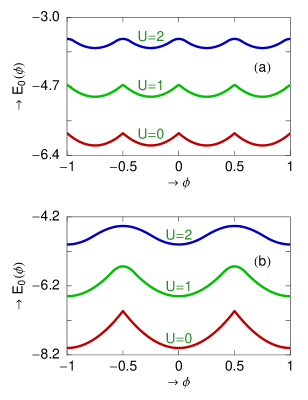
Figure 2: (Color online). Ground state energy levels as a function of flux $\phi$ for some typical mesoscopic rings in half-filled case. The red, green and blue curves correspond to $U=0$, $1$ and $2$, respectively. (a) $N=5$ and (b) $N=6$.

Hubbard strength $U$, while for all other cases traditional $\phi_{0}$ periodicity is obtained.

To judge the accuracy of the mean-field calculations in our ring geometry, in Fig. 3 we show the variation of lowest energy levels where the eigenenergies are determined through exact diagonalization of the full many-body Hamiltonian for the identical rings as given in Fig. 2, considering the same parameter values. Comparing the results presented in Figs. 2 and 3, we see that the mean-field results agree very well with the exact diagonalization method. Thus we can safely use mean-field approach to study magnetic response in our geometry.

III.1.2 Current-flux characteristics

Following the above energy-flux characteristics now we describe the behavior of persistent current in mesoscopic Hubbard rings. As representative examples, in Fig. 4 we display the variation of persistent currents as a function of flux $\phi$ for some typical single-channel mesoscopic rings in the half-filled case, where (a) and (b) correspond to $N=15$ and $20$, respectively. The red, green and blue curves in Fig. 4(a) correspond to the currents for $U=0$, $1.5$ and $2$, respectively, while these curves in Fig. 4(b) represent the currents for $U=0$, $1$ and $1.5$, respectively. In the absence of any e-e interaction ($U=0$), persistent current shows saw-tooth like nature as a function of flux $\phi$ with sharp transitions at $n\phi_{0}/2$ (red line of Fig. 4(a)) or $n\phi_{0}$ (red line of Fig. 4(b)), where $n$ being an integer, depending on whether $N$ is odd or even. The saw-tooth like behavior disappears as long as the electronic correlation is introduced into the system. This is clearly observed from the green and blue curves of Fig. 4. Additionally, in the presence of $U$, the current amplitude gets suppressed compared to the current amplitude in the non-interacting case, and it decreases gradually with increasing $U$. This provides the lowering of electron mobility with the rise of $U$ and the reason behind this can

Figure 3: (Color online). Ground state energy levels as a function of flux $\phi$ for some typical mesoscopic rings in half-filled case, where eigenenergies are determined through exact diagonalization of the full many-body Hamiltonian. The red, green and blue curves correspond to $U=0$, $1$ and $2$, respectively. (a) $N=5$ and (b) $N=6$.

be much better understood from our forthcoming discussion. Both for two different rings with sizes $N=15$ (odd) and $20$ (even), persistent currents vary periodically with AB flux $\phi$ showing different periodicities, following the energy-flux characteristics. For $N=15$, current shows $\phi_{0}/2$ flux-quantum periodicity, while for the other case ($N=20$), current exhibits $\phi_{0}$ flux-quantum periodicity.

III.1.3 Variation of electronic mobility: Drude weight

To reveal the conducting properties of Hubbard rings, we study the variation of Drude weight $D$ for these systems. Drude weight can be calculated by using Eq. 4. Finite value of $D$ predicts the metallic phase, while for the insulating phase it drops exponentially to zero kohn .

As illustrative examples, in Fig. 5 we show the variation of Drude weight $D$ as a function of electronic correlation strength $U$ for some typical single-channel Hubbard rings. In Fig. 5(a) the results are shown for three different half-filled rings, where the red, green and blue lines correspond to the rings with $N=10$, $30$ and $50$, respectively. From the curves it is evident that for smaller values of $U$, the half-filled rings show finite value of $D$ which reveals that they are in the metallic phase. On the other hand, $D$ drops sharply to zero when $U$ becomes high. Thus the rings become insulating when $U$ is quite large. The results for the non-half filled case are shown in Fig. 5(b), where we fix the ring size $N=20$ and vary the electron filling. The red, green and blue curves represent $N_{e}=10$, $14$ and $18$, respectively, where $N_{e}$ gives the total number of electrons in the ring. For these three choices of $N_{e}$,

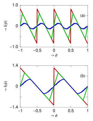
Figure 4: (Color online). Persistent current as a function of flux $\phi$ for single-channel mesoscopic rings in half-filled case. (a) $N=15$. The red, green and blue curves correspond to $U=0$, $1.5$ and $2$, respectively. (b) $N=20$. The red, green and blue curves correspond to $U=0$, $1$ and $1.5$, respectively.

the ring is always less than half-filled (since $N_{e}<N$) and the ring is in the conducting phase irrespective of the correlation strength $U$. Now we try to justify the dependence of the Hubbard strength $U$ on the electronic mobility for these different fillings. To understand the effect of $U$ on electron mobility here we measure a quantity called ‘average spin density’ (ASD) which is defined by the factor $\sum_{i}|(n_{i\uparrow}-n_{i\downarrow})|/N$. The integer $i$ is the site index and it runs from $1$ to $N$. By calculating ASD we can estimate the occupation probability of electrons in the ring and it supports us to explain whether the ring lies in the metallic phase or in the insulating one. For the rings those are below half-filled, ASD is always less than unity irrespective of the value of $U$ as shown by the curves in Fig. 6(b). It reveals that for these systems, ground state always supports an empty site and electron can move along the ring avoiding double occupancy of two different spin electrons at any site $i$ in the presence of e-e correlation which provides the metallic phase ($D>0$). For a fixed ring size and a particular strength of $U$, the ASD increases as the filling is increased towards half-filling which is noticed by comparing the three different curves in Fig. 6(b). On the other hand, in the half-filled rings, ASD is less than unity for small value of $U$, while it reaches to unity when $U$ is large. This behavior is clearly shown by the curves given in Fig. 6(a), where the red, green and blue lines correspond to ASDs for the half-filled rings with $N=10$, $30$ and $50$, respectively. Thus, for low $U$ there is some finite probability of getting two opposite

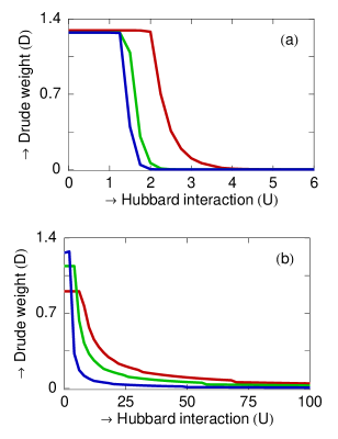
Figure 5: (Color online). Drude weight as a function of Hubbard interaction strength $U$ for single-channel mesoscopic rings. (a) Half-filled case. The red, green and blue curves correspond to $N=10$, $30$ and $50$, respectively. (b) Non-half-filled case with $N=20$. The red, green and blue curves correspond to $N_{e}=10$, $14$ and $18$, respectively.

spin electrons in a same site which allows electrons to move along the ring and the metallic phase is obtained. But for large $U$, ASD reaches to unity which means that each site is singly occupied either by an up or down spin electron with probability $1$. In this case ground state does not support any empty site and due to strong repulsive e-e correlation one electron sitting in a site does not allow to come other electron with opposite spin from the neighboring site which provides the insulating phase ($D=0$). The situation is somewhat analogous to Mott localization in one-dimensional infinite lattices. In perfect Hubbard rings the conducting nature has been studied exactly quite a long ago using the ansatz of Bethe by Shastry and Sutherland shastry . They have calculated charge stiffness constant ($D_{c}$) and have predicted that $D_{c}$ goes to zero as the system approaches towards half-filling for any non-zero value of $U$. Our numerical results clearly justify their findings.

III.1.4 Low-field magnetic susceptibility

Now, we discuss the variation of low-field magnetic susceptibility which can be calculated from Eq. 5 by setting $\phi\rightarrow 0$. With the help of this parameter we can justify whether the current is paramagnetic ($+$ve slope) or diamagnetic ($-$ve slope) in nature. For our illustrative purposes, in Fig. 7 we show the variation of low-field magnetic susceptibility with system size $N$ for some typical single-channel mesoscopic rings in the half-filled case. Figure 7(a) correspond to the variation

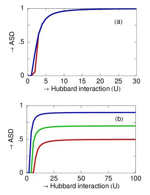
Figure 6: (Color online). Average spin density (ASD) as a function of Hubbard interaction strength $U$ for single-channel mesoscopic rings. (a) Half-filled case. The red, green and blue curves correspond to $N=10$, $30$ and $50$, respectively. (b) Non-half-filled case with $N=20$. The red, green and blue curves correspond to $N_{e}=10$, $14$ and $18$, respectively.

of low-field magnetic susceptibility for the non-interacting ($U=0$) rings, where the ring size can by anything i.e., either odd, following the relation $N=2n+1$ ($n$ is an integer), or even, obeying the expression $N=2n+2$. It is observed that both for odd and even $N$, low-field current exhibits diamagnetic nature. The behavior of the low-field currents changes significantly when the e-e interaction is taken into account. Depending on the ring size $N$, the sign becomes $+$ve and $-$ve as shown by the curves given in Figs. 7(b)-(d). For the interacting rings where the relation $N=4n+2$ is satisfied, the low-field current becomes diamagnetic (Fig. 7(b)). The sign becomes paramagnetic when $N=4n$ (Fig. 7(c)) and $N=2n+1$ (Fig. 7(d)). Thus, in brief, we say that for non-interacting half-filled rings low-field current exhibits diamagnetic response irrespective of $N$ i.e., whether $N$ is odd or even. For the interacting half-filled rings with odd $N$, low-field current provides only the paramagnetic behavior, while for even $N$, depending on the particular value of $N$, the response becomes either diamagnetic or paramagnetic. These natures of low-field currents change for the cases of other electron fillings. Hence, it can be emphasized that the behavior of the low-field currents is highly sensitive on the Hubbard correlation, electron filling, evenness and oddness of $N$, etc. The behavior of zero-field magnetic susceptibility in Hubbard rings has been studied extensively quite a long back using the Bethe ansatz by Shiba shiba . In this work, he has studied magnetic

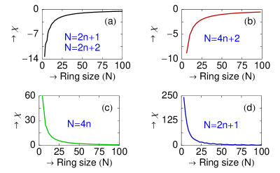
Figure 7: (Color online). Low-field magnetic susceptibility as a function of system size $N$ for single-channel mesoscopic rings in half-filled case. (a) $U=0$. $N$ is an odd ($2n+1$) or an even ($2n+2$) number, where $n$ is an integer. (b) $U=1$. $N$ is an even number obeying the relation $N=4n+2$. (c) $U=1$. $N$ is an even number satisfying the relation $N=4n$. (d) $U=1$. $N$ is an odd number following the relation $N=2n+1$.

susceptibility per electron as functions of electron filling and Hubbard correlation strength and provided several interesting results. From his findings we can clearly justify our presented results.

III.2 Disordered Hubbard Rings Described with NNH and SNH Integrals

Finally, we explore the combined effect of electron-electron correlation and second-neighbor hopping (SNH) integral on persistent current in disordered mesoscopic rings.

To get a disordered ring, we choose site energies ($\epsilon_{i\uparrow}$ and $\epsilon_{i\downarrow}$) randomly from a “Box” distribution function of width $W$. As the site energies are chosen randomly it is needed to consider the average over a large number of disordered configurations (from the stand point of statistical average). Here, we determine the currents by taking the average over $50$ random disordered configuration in each case to achieve much accurate results.

As illustrative examples, in Fig. 8 we display the variation of persistent currents for some single-channel mesoscopic rings considering $1/3$ electron filling. In (a) the results are given for the rings characterized by the NNH integral model. The red curve represents the current for the ordered ($W=0$) non-interacting ($U=0$) ring. It shows saw-tooth like nature with AB flux $\phi$ providing $\phi_{0}$ flux-quantum periodicity. The situation becomes completely different when impurities are introduced in the ring as clearly seen by the other two colored curves. The green curve represents the current for the case only when impurities are considered but the effect of Hubbard interaction is not taken into account. It varies continuously with $\phi$ and gets much reduced amplitude, even an order of magnitude, compared to the perfect case. This is due to the localization of the energy eigenstates in the presence of impurity, which is the so-called Anderson localization. Hence, a large difference exists between the current amplitudes of an ordered and disordered non-interacting rings and it was the main controversial issue among the theoretical and experimental predictions. Experimental results suggest that the measured current amplitude is quite comparable to the theoretically estimated current amplitude in a perfect system. To remove this controversy, as a first attempt, we include the effect of Hubbard interaction in the disordered ring described by the NNH model. The result is shown by the blue curve where $U$ is fixed at $0.5$. It is observed that the current amplitude gets increased compared to the non-interacting disordered ring, though the increment is too small. Not only that the enhancement can take place only for small values of $U$, while for large enough $U$ the current amplitude rather decreases. This phenomenon can be explained as follows. For the non-interacting disordered ring the probability of getting two opposite spin electrons becomes higher at the atomic sites where the site energies are lower than the other sites since the electrons get pinned at the lower site energies to minimize the ground state energy, and this pinning of electrons becomes increased with the rise of impurity strength $W$. As a result the mobility of electrons and hence the current amplitude gets reduced with the increase of impurity strength $W$. Now, if we introduce electronic correlation in the system then it tries to depin two opposite spin electrons those are situated together due to the Coulomb repulsion. Therefore, the electronic mobility is enhanced which provides quite larger current amplitude. But, for large enough interaction strength, mobility of electrons gradually decreases due to the strong repulsive interaction. Accordingly, the current amplitude gradually decreases with $U$. So, in short, we can say that within the nearest-neighbor hopping (NNH) model electron-electron interaction does not provide any significant contribution to enhance the current amplitude, and hence the controversy regarding the current amplitude still persists.

To overcome this controversy, finally we make an attempt by incorporating the effect of second-neighbor hopping (SNH) integral in addition to the nearest-neighbor hopping (NNH) integral. With this modification a significant change in current amplitude takes place which is clearly observed from Fig. 8(b). The red curve refers to the current for the perfect ($W=0$) non-interacting ($U=0$) ring and it achieves much higher amplitude compared to the NNH model (see red curve of Fig. 8(a)). This additional contribution comes from the SNH integral since it allows electrons to hop further.

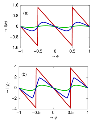
Figure 8: (Color online). Persistent current as a function of flux $\phi$ for single-channel mesoscopic rings with $N=15$ considering $1/3$ electron filling. (a) Rings with only NNH integral. The red line corresponds to the ordered non-interacting ring, while the green and blue lines correspond to the disordered ($W=2$) rings with $U=0$ and $0.5$, respectively. (b) Rings with NNH and SNH integrals. The red line represents the ordered non-interacting ring, whereas the green and blue line correspond to the disordered ($W=2$) rings with $U=0$ and $1.5$, respectively.

The main focus of this sub-section is to interpret the combined effect of SNH integral and Hubbard correlation on the enhancement of persistent current in disordered ring. To do this first we narrate the effect of SNH integral in disordered non-interacting ring. The nature of the current for this particular case is shown by the green curve of Fig. 8(b). It shows that the current amplitude gets reduced compared to the perfect case (red line), which is expected, but the reduction of the current amplitude is very small than the NNH integral model (see green curve of Fig. 8(a)). This is due the fact that the SNH integral tries to delocalize the electronic states, and therefore, the mobility of the electrons is enriched. The situation becomes more interesting when we include the effect of Hubbard interaction. The behavior of the current in the presence of interaction is plotted by the blue curve of Fig. 8(b) where we fix $U=1.5$. Very interestingly we see that the current amplitude is enhanced moderately and quite comparable to that of the perfect cylinder. Therefore, it can be predicted that the presence of SNH integral and Hubbard interaction can provide a persistent current which may be comparable to the measured current amplitudes. In this presentation we consider the effect of only SNH integral in addition to the NNH model, and, illustrate how such a higher order hopping integral leads an important role on the enhancement of current amplitude in presence of Hubbard correlation for disordered rings. Instead of considering only the SNH integral we can also take the contributions from all possible higher order hopping integrals with reduced hopping strengths. Since the strengths of other higher order hopping integrals are too small, the contributions from these factors are reasonably small and they will not provide any significant change in the current amplitude. Finally, we can say that further studies are needed by incorporating all these factors.

IV Closing remarks

To summarize, we have studied magnetic response in mesoscopic Hubbard rings threaded by Aharonov-Bohm flux $\phi$. Using the generalized Hartree-Fock (HF) approximation, we have numerically computed persistent current, Drude weight, low-field magnetic susceptibility and some other related issues. Most importantly, we have tried to implement an idea to remove the long standing problem between the experimentally measured and theoretically predicted current amplitudes. We believe the present analysis is found to exhibit several interesting results which have so far remained unaddressed.

ACKNOWLEDGMENTS

I acknowledge with deep sense of gratitude the illuminating comments and suggestions I have received from Prof. Shreekantha Sil, Prof. S. N. Karmakar, Prof. Bibhas Bhattacharyya, Srilekha Saha and Moumita Dey during the calculations.

References

- (1) M. Büttiker, Y. Imry, and R. Landauer, Phys. Lett. 96A, 365 (1983).
- (2) L. P. Levy, G. Dolan, J. Dunsmuir, and H. Bouchiat, Phys. Rev. Lett. 64, 2074 (1990).
- (3) V. Chandrasekhar, R. A. Webb, M. J. Brady, M. B. Ketchen, W. J. Gallagher, and A. Kleinsasser, Phys. Rev. Lett. 67, 3578 (1991).
- (4) E. M. Q. Jariwala, P. Mohanty, M. B. Ketchen, and R. A. Webb, Phys. Rev. Lett. 86, 1594 (2001).
- (5) R. Deblock, R. Bel, B. Reulet, H. Bouchiat, and D. Mailly, Phys. Rev. Lett. 89, 206803 (2002).
- (6) H. F. Cheung, Y. Gefen, E. K. Riedel, and W. H. Shih, Phys. Rev. B 37, 6050 (1988).
- (7) H. F. Cheung, E. K. Riedel, and Y. Gefen, Phys. Rev. Lett. 62, 587 (1989).
- (8) L. K. Castelano, G.-Q. Hai, B. Partoens, and F. M. Peeters, Phys. Rev. B 78, 195315 (2008).
- (9) M. Zarenia, M. J. Pereira, F. M. Peeters, and G. de Farias, Phys. Rev. B 81, 045431 (2010).
- (10) D. Y. Vodolazov, F. M. Peeters, T. T. Hongisto, and K. Yu. Arutyunov, Europhys. Lett. 75, 315 (2006).
- (11) G. Montambaux, H. Bouchiat, D. Sigeti, and R. Friesner, Phys. Rev. B 42, 7647 (1990).
- (12) B. L. Altshuler, Y. Gefen, and Y. Imry, Phys. Rev. Lett. 66, 88 (1991).
- (13) F. von Oppen and E. K. Riedel, Phys. Rev. Lett. 66, 84 (1991).
- (14) A. Schmid, Phys. Rev. Lett. 66, 80 (1991).
- (15) V. Ambegaokar and U. Eckern, Phys. Rev. Lett. 65, 381 (1990).
- (16) G. Bouzerar, D. Poilblanc, and G. Montambaux, Phys. Rev. B 49, 8258 (1994).
- (17) T. Giamarchi and B. S. Shastry, Phys. Rev. B 51, 10915 (1995).
- (18) N. Yu and M. Fowler, Phys. Rev. B 45, 11795 (1992).
- (19) S. K. Maiti, J. Chowdhury, and S. N. karmakar, Phys. Lett. A 332, 497 (2004).
- (20) S. K. Maiti, J. Chowdhury, and S. N. karmakar, J. Phys.: Condens. Matter 18, 5349 (2006).
- (21) S. K. Maiti, Physica E 31, 117 (2006).
- (22) S. K. Maiti, Solid State Phenomena 155, 87 (2009).
- (23) H. Kato and D. Yoshioka, Phys. Rev. B 50, 4943 (1994).
- (24) A. Kambili, C. J. Lambert, and J. H. Jefferson, Phys. Rev. B 60, 7684 (1999).
- (25) S. Gupta, S. Sil, and B. Bhattacharyya, Physica B 355, 299 (2005).
- (26) W. Kohn, Phys. Rev. 133, A171 (1964).
- (27) B. S. Shastry and B. Sutherland, Phys. Rev. Lett. 65, 243 (1990).
- (28) H. Shiba, Phys. Rev. B 6, 930 (1972).