Sensitivity of Antenna Arrays for Long-Wavelength Radio Astronomy

Abstract

A number of new and planned radio telescopes will consist of large arrays of low-gain antennas operating at frequencies below 300 MHz. In this frequency regime, Galactic noise can be a significant or dominant contribution to the total noise. This, combined with mutual coupling between antennas, makes it difficult to predict the sensitivity of these instruments. This paper describes a system model and procedure for estimating the system equivalent flux density (SEFD) – a useful and meaningful metric of the sensitivity of a radio telescope – that accounts for these issues. The method is applied to LWA-1, the first “station” of the Long Wavelength Array (LWA) interferometer. LWA-1 consists of 512 bowtie-type antennas within a 110 $\times$ 100 m elliptical footprint, and is designed to operate between 10 MHz and 88 MHz using receivers having noise temperature of about 250 K. It is shown that the correlation of Galactic noise between antennas significantly desensitizes the array for beam pointings which are not close to the zenith. It is also shown that considerable improvement is possible using beamforming coefficients which are designed to optimize signal-to-noise ratio under these conditions. Mutual coupling is found to play a significant role, but does not have a consistently positive or negative influence. In particular, we demonstrate that pattern multiplication (assuming the behavior of single antennas embedded in the array is the same as those same antennas by themselves) does not generate reliable estimates of SEFD.

I Introduction

A number of new and planned radio telescopes will consist of large arrays of closely-spaced low-gain antennas operating at frequencies below 300 MHz. These include LWA [1], LOFAR [2], MWA [3], and SKA [4]. In this frequency regime, it is possible to design receivers with noise temperatures that are much less than the antenna temperatures associated with the ubiquitous Galactic synchrotron radiation, such that the resulting total system noise temperature is dominated by Galactic noise [5]. This is quite different from the condition most often considered, in which it is usually assumed that internal noise associated with the receivers dominates and does not scatter into the array, so that the noise associated with different antennas is uncorrelated; see e.g. [6, 7, 8]. Recent work on arrays for long-wavelength radio astronomy accounts for the dominance of external noise, but neglects the effects of correlation of this noise between antennas [9, 1]. However, it is known that this correlation is likely to have a significant effect for these instruments [10], and this issue is further explored in this paper. In [11, 12], and [13], correlation of noise between antennas is considered, but the source of noise is internal (amplifiers or ohmic losses in antennas) and the correlation arises due to propagation internal to the array. The problem of correlation of external noise has been intermittently considered in communications (e.g. [14]) and direction finding (e.g. [15]) applications, but does not seem to have been previously considered for long-wavelength radio astronomy beamforming applications.

Because antenna spacing in the systems of interest is typically less than a few wavelengths, mutual coupling also plays a significant role. Since these arrays are electromagnetically large, interact with the electromagnetically-complex ground, and may have aperiodic spacings, it is difficult to determine the characteristics of antennas, either individually or collectively as part of a beamforming system. In particular, it is usually difficult to know if pattern multiplication – that is, assuming that the behavior of single antennas embedded in the array is the same as those same antennas by themselves – yields reasonable results. Past studies have shown that mutual coupling in aperiodic arrays of low-gain elements results in fluctuation of beam gain and sidelobe levels as a function of scan angle when element spacing is less than a few wavelengths [16, 17]. This suggests that pattern multiplication may not be a useful assumption. However, useful and generalizable findings which are applicable to the systems of interest are not commonly available.

This paper describes a procedure for estimating the sensitivity of radio telescope arrays which is appropriate under these conditions. The procedure is based on a system model, described in Section II, which relates the electromagnetic response of the array (the array manifold), a model for the external noise temperature, and a model for the receiver noise temperatures to the system equivalent flux density (SEFD) achieved by a beam formed using specified beamforming coefficients. SEFD is defined as the power flux spectral density (i.e., W m^-2 Hz^-1) which yields signal-to-noise ratio (SNR) equal to unity at the beamformer output. SEFD is a useful metric as it includes the combined effect of antennas and all noise sources into a single “bottom line” number that is directly related to the sensitivity of astronomical observations.

The primary difficulty in determining SEFD using the above procedure is obtaining the array manifold. One approach is demonstrated by example in Section III of this paper. We analyze LWA-1, the first “station” of the Long Wavelength Array (LWA) interferometer [1]. LWA-1 consists of 512 bowtie-type antenna elements arranged into 256 dual-polarized “stands” within a 110 $\times$ 100 m elliptical footprint. LWA-1 is designed to operate between 10 MHz and 88 MHz using receivers having noise temperature of about 250 K. We obtain the array manifold for LWA-1 at 20 MHz, 38 MHz, and 74 MHz using a method of moments (MoM) wire-grid model. Because the model is too large to analyze all at once (a common problem with this class of arrays), a procedure described in Section III-B is employed in which the manifold is calculated for one stand (i.e., one pair of collocated antenna elements) at a time. Unlike pattern multiplication in which the presence of the remaining stands would be ignored, this procedure obtains the response of each antenna in the presence of nearby antennas and structures.

Also considered in this paper is the selection and performance of beamforming coefficients which optimize SEFD. Because mutual coupling and external noise correlation are significant, it is to be expected that “simple” beamforming coefficients based solely on antenna positions (i.e., phases associated with geometry only) will not be optimal. In Section IV, the SEFD performance of LWA-1 is evaluated. It is shown that the optimal coefficients significantly improve sensitivity relative to simple coefficients. Finally, in Section V, the extension of these results to predict the imaging performance of an interferometer comprised of multiple beamforming arrays is considered.

II Theory

Let $E_{\theta}(t)$ and $E_{\phi}(t)$ be the $\theta$- and $\phi$-polarized components of the electric field of the signal of interest, having units V m^-1 Hz^-1/2. In this coordinate system, $\theta$ is measured from the $+z$ axis, which points toward the zenith; the ground lies in the $z=0$ plane, and $\phi$ is measured from the $+x$ axis. The signal of interest is incident from $\{\theta_{0},\phi_{0}\}$, which is henceforth indicated as $\psi_{0}$. The resulting voltage across the terminals of the $n^{\mbox{th}}$ antenna element, having units of V Hz^-1/2, is

$$x_{n}(t)=a^{\theta}_{n}(\psi_{0})E_{\theta}(t)+a^{\phi}_{n}(\psi_{0})E_{\phi}(t)+z_{n}(t)+u_{n}(t)$$ (1)

where: $a^{\theta}(\psi_{0})$ and $a^{\phi}(\psi_{0})$ are the effective lengths, having units of meters, associated with the $\theta$ and $\phi$ polarizations, respectively, for the $n^{\mbox{th}}$ antenna element for signals incident from $\psi_{0}$; $z_{n}(t)$ is the contribution from noise external to the system; and $u_{n}(t)$ is the contribution from noise internal to the system. Note $u_{n}(t)$ can also include internal noise unintentionally radiated by some other antenna and received by antenna $n$. In all cases, we assume these quantities are those which apply when antennas are terminated into whatever electronics are actually employed in the system, as opposed to being “open circuit” or “short circuit” quantities. Without loss of generality we can interpret these to be time-harmonic (i.e., monochromatic complex-valued “baseband”) quantities.

Beamforming can be described as the operation:

$$y(t)=\sum_{n=1}^{N}{b_{n}x_{n}(t)}$$ (2)

where $N$ is the number of antennas, and the unitless $b_{n}$’s specify the beam. Assuming root-mean-square voltages, the power at the output of the beamformer is

$$P_{y}=\left<y(t)y^{*}(t)\right>R_{o}^{-1}$$ (3)

where $<\cdot>$ denotes time-domain averaging and “^∗” denotes conjugation, and $R_{o}$ is the impedance looking into the system as seen from the terminals across which $y(t)$ is measured, assumed to be purely resistive.

We now wish to evaluate Equation 3 by substitution of Equation 2. In the process of expanding Equation 3, let us assume that the signal of interest, $z_{n}(t)$, and $u_{n}(t)$ are mutually uncorrelated for any given $n$. Specifically, we assume that for any $n$ and $m$:

$$\left<E_{\theta}(t)z_{n}^{*}(t)\right>=\left<E_{\phi}(t)z_{n}^{*}(t)\right>=0$$ (4)

$$\left<E_{\theta}(t)u_{n}^{*}(t)\right>=\left<E_{\phi}(t)u_{n}^{*}(t)\right>=0$$ (5)

$$\left<z_{n}(t)u_{m}^{*}(t)\right>=0~{}\mbox{.}$$ (6)

Note that the possibility that like terms are correlated between antennas is not precluded by the above assumptions; for example, $\left<z_{n}(t)z_{m}^{*}(t)\right>$ can be $\neq 0$ for $n\neq m$. Furthermore, we have not yet made any assumption about the correlation between $E_{\theta}(t)$ and $E_{\phi}(t)$. Under these assumptions, Equation 3 can be written as follows:

$$P_{y}R_{o}= {\bf b}^{H}{\bf A}_{\theta\theta}{\bf b}~{}P_{\theta\theta}+{\bf b}^{H}{\bf A}_{\phi\phi}{\bf b}~{}P_{\phi\phi}$$ (7)

$$+ {\bf b}^{H}{\bf A}_{\theta\phi}{\bf b}~{}P_{\theta\phi}+{\bf b}^{H}{\bf A}_{\phi\theta}{\bf b}~{}P_{\phi\theta}$$

$$+ {\bf b}^{H}{\bf P}_{z}{\bf b}~{}~{}~{}~{}~{}~{}~{}+{\bf b}^{H}{\bf P}_{u}{\bf b}~{}\mbox{,}$$

where “^H” denotes the conjugate transpose operator;

$${\bf b}=\left[~{}b_{1}~{}b_{2}~{}\cdots~{}b_{N}~{}\right]^{T}~{}\mbox{,}$$ (8)

where “^T” denotes the transpose operator; and

$${\bf A}_{\theta\theta}={\bf a}_{\theta}^{*}(\psi_{0})~{}{\bf a}_{\theta}^{T}(\psi_{0})~{}~{}~{}P_{\theta\theta}=\left<\left|E_{\theta}(t)\right|^{2}\right>~{}~{}$$ (9)

$${\bf A}_{\phi\phi}={\bf a}_{\phi}^{*}(\psi_{0})~{}{\bf a}_{\phi}^{T}(\psi_{0})~{}~{}~{}P_{\phi\phi}=\left<\left|E_{\phi}(t)\right|^{2}\right>~{}~{}$$ (10)

$${\bf A}_{\theta\phi}={\bf a}_{\phi}^{*}(\psi_{0})~{}{\bf a}_{\theta}^{T}(\psi_{0})~{}~{}~{}P_{\theta\phi}=\left<E_{\theta}(t)E_{\phi}^{*}(t)\right>$$ (11)

$${\bf A}_{\phi\theta}={\bf a}_{\theta}^{*}(\psi_{0})~{}{\bf a}_{\phi}^{T}(\psi_{0})~{}~{}~{}P_{\phi\theta}=\left<E_{\phi}(t)E_{\theta}^{*}(t)\right>$$ (12)

$${\bf a}_{\theta}(\psi_{0})=\left[~{}a_{1}^{\theta}(\psi_{0})~{}a_{2}^{\theta}(\psi_{0})~{}\cdots~{}a_{N}^{\theta}(\psi_{0})~{}\right]^{T}$$ (13)

$${\bf a}_{\phi}(\psi_{0})=\left[~{}a_{1}^{\phi}(\psi_{0})~{}a_{2}^{\phi}(\psi_{0})~{}\cdots~{}a_{N}^{\phi}(\psi_{0})~{}\right]^{T}~{}\mbox{;}$$ (14)

and ${\bf P}_{z}$ is a matrix whose $(n,m)^{\mbox{th}}$ element is $\left<z_{n}^{*}(t)z_{m}(t)\right>$, and ${\bf P}_{u}$ is a matrix whose $(n,m)^{\mbox{th}}$ element is $\left<u_{n}^{*}(t)u_{m}(t)\right>$.

We now consider the external noise correlation matrix ${\bf P}_{z}$. We wish to obtain a simple expression for ${\bf P}_{z}^{\left[n,m\right]}$, the $\left(n,m\right)^{\mbox{th}}$ element of ${\bf P}_{z}$, in terms of physical quantities more relevant to radio astronomy. First, let us define $\Delta S(\psi)$ as the flux density, having units of W m^-2 Hz^-1, associated with the electric field $\Delta E(\psi,t)$ incident from a region of solid angle $\Delta\Omega$ around $\psi$. Assuming $\Delta E(\psi,t)$ is given in terms of root-mean-square voltage, the relationship is

$$\Delta S(\psi)=\left<\left|\Delta E(\psi,t)\right|^{2}\right>/\eta$$ (15)

where $\eta$ is the impedance of free space. Since the Galactic synchrotron background noise is essentially unpolarized, we assume the powers in the $\theta$- and $\phi$-polarized components of $\Delta E(\psi,t)$ are equal; specifically,

$$\left<\left|\Delta E_{\theta}(\psi,t)\right|^{2}\right>=\left<\left|\Delta E_{\phi}(\psi,t)\right|^{2}\right>=\frac{\eta}{2}\Delta S(\psi)$$ (16)

Note also that $\Delta S(\psi)$ can be obtained independently from the Rayleigh-Jeans Law:

$$\Delta S(\psi)=\frac{2k}{\lambda^{2}}T_{e}(\psi)\Delta\Omega$$ (17)

where $k$ is Boltzmann’s constant ($1.38\times 10^{-23}$ J/K), $T_{e}(\psi)$ is the apparent external noise brightness temperature (attributable to either Galactic noise or thermal radiation from the ground) in the direction $\psi$, and $\lambda$ is wavelength. We can model $\Delta E_{\theta}(\psi,t)$ and $\Delta E_{\phi}(\psi,t)$ as follows:

$$\Delta E_{\theta}(\psi,t)=g_{\theta}(\psi,t)\sqrt{\frac{k\eta}{\lambda^{2}}T_{e}(\psi)\Delta\Omega}$$ (18)

$$\Delta E_{\phi}(\psi,t)=g_{\phi}(\psi,t)\sqrt{\frac{k\eta}{\lambda^{2}}T_{e}(\psi)\Delta\Omega}$$ (19)

where $g_{\theta}(\psi,t)$ and $g_{\phi}(\psi,t)$ are Gaussian-distributed random variables with zero mean and unit variance. Note that we expect not only that $g_{\theta}(\psi,t)$ and $g_{\phi}(\psi,t)$ will be independent random variables, but also that $g_{\theta}(\psi_{1},t)$ and $g_{\theta}(\psi_{2},t)$ will be uncorrelated for $\psi_{1}\neq\psi_{2}$, and similarly for $g_{\phi}(\psi,t)$. We obtain $z_{n}(t)$ by summing up the contributions received over a sphere:

$$z_{n}(t)=\sum_{\psi}{\left[a^{\theta}_{n}(\psi)\Delta E_{\theta}(\psi,t)+a^{\phi}_{n}(\psi)\Delta E_{\phi}(\psi,t)\right]}$$ (20)

Applying the definition of ${\bf P}_{z}$ and exploiting the statistical properties of $g_{\theta}(\psi,t)$ and $g_{\phi}(\psi,t)$, we find:

$${\bf P}_{z}^{\left[n,m\right]}=\\ \frac{k\eta}{\lambda^{2}}\sum_{\psi}{\left[a^{\theta*}_{n}(\psi)a^{\theta}_{m}(\psi)+a^{\phi*}_{n}(\psi)a^{\phi}_{m}(\psi)\right]T_{e}(\psi)\Delta\Omega}$$ (21)

which can now be written in integral form:

$${\bf P}_{z}^{\left[n,m\right]}=\\ \frac{k\eta}{\lambda^{2}}\int{\left[a^{\theta*}_{n}(\psi)a^{\theta}_{m}(\psi)+a^{\phi*}_{n}(\psi)a^{\phi}_{m}(\psi)\right]T_{e}(\psi)d\Omega}$$ (22)

Returning to Equation 7, note that the signal to noise ratio (SNR) at the output of the beamformer can be written as:

$$\mbox{SNR}=\frac{{\bf b}^{H}{\bf R}_{s}{\bf b}}{{\bf b}^{H}{\bf R}_{n}{\bf b}}~{}\mbox{,}$$ (23)

where

$${\bf R}_{s}={\bf A}_{\theta\theta}P_{\theta\theta}+{\bf A}_{\phi\phi}P_{\phi\phi}+{\bf A}_{\theta\phi}P_{\theta\phi}+{\bf A}_{\phi\theta}P_{\phi\theta}~{}\mbox{, and}$$ (24)

$${\bf R}_{n}={\bf P}_{z}+{\bf P}_{u}~{}\mbox{.}$$ (25)

In general, the maximum possible SNR is equal to the maximum eigenvalue of ${\bf R}_{n}^{-1}{\bf R}_{s}$, and is achieved by selecting ${\bf b}$ to be the corresponding eigenvector [18] (see also [6]). Alternative approaches to beamforming include (1) selecting ${\bf b}={\bf a}_{\theta}^{*}(\psi_{0})$ or ${\bf a}_{\phi}^{*}(\psi_{0})$, which accounts for mutual coupling but neglects spatial noise correlation; or (2) selecting the beamforming coefficients to compensate only for the geometrical delays, which neglects both effects. Approach (1) is optimal when the noise associated with each antenna is uncorrelated, such that ${\bf R}_{n}$ has the form $\sigma_{n}^{2}{\bf I}$; i.e., some constant times the identity matrix. Then, we obtain the well-known result that the SNR improves linearly with $N$. However, as will be demonstrated in later in this paper, this special case is not necessarily relevant to the problem of interest. This is primarily due to the impact of the external noise correlation, as represented by ${\bf P}_{z}$, for which off-diagonal terms can be significant.

For a signal of interest which is unpolarized – a useful and common assumption for the purpose of characterizing the sensitivity of a radio telescope – we have $P_{\theta\phi}=P_{\phi\theta}=0$ and $P_{\theta\theta}=P_{\phi\phi}=\eta S(\psi)/2$, where $S(\psi)$ is the flux (distinct from the external noise considered above) associated with the signal of interest. In this case, we have

$${\bf R}_{s}=S(\psi)\frac{\eta}{2}\left({\bf A}_{\theta\theta}+{\bf A}_{\phi\phi}\right)~{}\mbox{.}$$ (26)

Continuing with this assumption, it is convenient to express the sensitivity of a radio telescope in terms of system equivalent flux density (SEFD), defined as the value of $S(\psi)$ in Equation 26 required to double the total power observed at the beamformer output; i.e., SNR$=$1. Thus,

$$\mbox{SEFD}=\frac{2}{\eta}\frac{{\bf b}^{H}\left({\bf P}_{z}+{\bf P}_{u}\right){\bf b}}{{\bf b}^{H}\left({\bf A}_{\theta\theta}+{\bf A}_{\phi\phi}\right){\bf b}}~{}\mbox{.}$$ (27)

This expression is useful as it describes the sensitivity of a radio telescope array in terms of the array manifold, the contributions of internal and external noise, and the beamforming coefficients. The principal difficulty in using this expression is calculating the array manifold. This is considered next.

III LWA-1 Design and Array Manifold

The original motivation behind the work presented in this paper was to characterize the performance of LWA-1. LWA-1 consists of $N=512$ antennas arranged into 256 “stands”, with each stand consisting of two orthogonally-aligned bowtie-type dipoles over a wire mesh ground screen, as shown in Figure 1. In Sections III-A and III-B we review the relevant details of the design of the LWA-1 array, our method for computing the array manifold and the internal and external noise covariance matrices, and present some results.

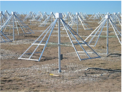
Figure 1: LWA-1 under construction (picture taken November 2009), showing a few of the completed stands.

III-A LWA Stand Design & Electromagnetic Model

As the dipoles and ground screen comprising each stand consist of interconnected metal segments, the array is well-suited to wire grid modeling using the Method of Moments (MoM). In this study, we employ the NEC-4.1 implementation of MoM [19].

The dimensions and parameters used to model the dipole are illustrated in Figure 2. The wire grid models representing each of the two antennas in a stand are vertically separated by three times the wire radius to prevent the feeds from intersecting. The mean height of the highest points on each dipole (also the segment containing the feed) is 1.5 m above ground. It is known from both simulations and experiment that neither the center mast nor the structure supporting the dipole arms (see Figure 1) have a significant effect on the relevant properties of the dipoles, and therefore no attempt is made to model them. It should be noted that the segmentation shown in Figure 2 is designed to be valid for the highest frequency of interest, so that the same model can be used for all frequencies of interest. In order to confirm that the results were not sensitive to the selected segmentation, several alternative schemes with small changes in the number of segments per wire were also considered. The results do not change significantly with these changes in segmentation.

The ground screen is modeled using a 3 m $\times$ 3 m wire grid with spacing 10 cm $\times$ 10 cm and wire radius of 1 mm, which is very close to the actual dimensions. The modeled ground screen is located 1 cm above ground to account for the significant but irregular gap that exists because of ground roughness. The ground itself is modeled as an infinite homogeneous half-space with relative permittivity of 3 and conductivity of 100 $\mu$S, which is appropriate for “very dry ground” [20] which predominates in New Mexico, where LWA-1 is located. (It should be noted that we suspect that the ground permittivity at the LWA-1 site is significantly higher; this is addressed below.) Each dipole is connected to an active balun which presents a balanced input impedance of $R_{L}=100~{}\Omega$. For additional information on this design, the reader is referred to [1] and the references therein.

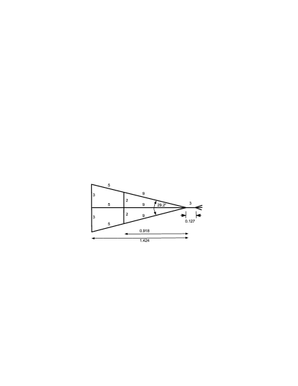
Figure 2: Geometry of the wire grid used to model the dipole. Dimensions are in meters. The number of segments used in the MoM model are indicated next to each wire. The radius of all wires is 1.2 cm, modeling aluminum tubing having square cross-section with 3/4-in sides. The dipole arms are bent $45^{\circ}$ downward from the junction with the center (feed) wire.

It will be useful later in this paper to know the performance of a single stand, neglecting the rest of the array. We begin with the array manifold for the stand, which is determined as follows. The stand is illuminated with a $\theta$-polarized 1 V/m plane wave incident from some direction $\psi$, and the resulting current $I_{L}$ across the series resistance modeling each active balun is determined using MoM. Each element of the $N=2$ array response vector ${\bf a}_{\theta}(\psi)$ is then simply $I_{L}R_{L}$ for the associated antenna. The process is repeated for a $\phi$-polarized plane wave and iterated over $\psi$.

The external noise covariance matrix ${\bf P}_{z}$ is computed using a model proposed in [5] which assumes that Galactic noise dominates over thermal noise from the ground and other natural or anthropogenic sources of noise. Specifically, $T_{e}(\psi)$ is assumed to be uniform over the sky ($\theta<\pi/2$), and zero for $\theta>\pi/2$. In practice, $T_{e}(\psi)$ varies considerably both as a function of $\psi$ and as a function of time of day, due to the rotation of the Earth. However, the above assumption provides a reasonable standard condition for comparing Galactic noise-dominated antenna systems, as explained in [5] and demonstrated in [21] and [22]. Using this model, $T_{e}(\psi)$ toward the sky is found to be 50,444 K, 9751 K, and 1777 K at 20 MHz, 38 MHz, and 74 MHz, respectively. The actual contributions to the system temperature are less due to the mismatch between the antenna self-impedance and $R_{L}$, but this is automatically taken into account as a consequence of our definition of the array manifold, which includes the loss due to impedance mismatch as well as ground loss. Under these assumptions, ${\bf P}_{z}$ is computed using Equation 22.

The internal noise covariance matrix ${\bf P}_{u}$ is computed assuming that the internal noise associated with any given antenna is not significantly correlated with the internal noise associated with any other antenna, so that ${\bf P}_{u}$ becomes a diagonal matrix whose non-zero elements are:

$${\bf P}_{u}^{\left[n\right]}=kT_{p,n}R_{L}$$ (28)

where $T_{p,n}$ is the input-referred internal noise temperature associated with the $n^{\mbox{th}}$ antenna. We will further assume that all the electronics are identical such that $T_{p,n}=T_{p}$, where $T_{p}$ is assumed to be $250$ K, the nominal value of the cascade noise temperature of all electronics attached to a dipole, referred to the dipole terminals.

The ratio $Tr\left\{{\bf P}_{z}\right\}/Tr\left\{{\bf P}_{u}\right\}$ (where “$Tr$” denotes the trace operation; i.e., the sum of the diagonal elements) is the degree to which Galactic noise dominates over internal noise in the combined output, and is found to be $-2.6$ dB, $+11.1$ dB, and $+4.1$ dB at 20, 38, and 74 MHz, respectively. The 38 MHz and 74 MHz results are consistent with field measurements (see Figure 6 of [1]), however the same measurements suggest 20 MHz should also be Galactic noise-dominated. The apparent reason for the discrepancy is that the 20 MHz result is relatively sensitive to ground permittivity, both because the loss associated with Earth ground increases with decreasing frequency, and also because the ground screen becomes tiny (only $0.2\lambda\times 0.2\lambda$) at 20 MHz. Larger assumed permittivity in our calculations results in Galactic noise-dominated performance at 20 MHz, even if the loss tangent is also increased. The effect of the change of ground parameters on the 38 MHz and 74 MHz results is very small in comparison. We shall continue to use the original ground parameters in this paper as they can be considered to be safely conservative.

Using the array manifold and the noise covariance matrices calculated as described above, the resulting SEFD for a single stand (and neglecting the rest of the array) can be computed from Equation 27. The result for the $\phi=0$ plane is shown in Figure 3. Note Figure 3 is also essentially a pattern measurement; as such the expected “$\cos{\theta}$”-type behavior is evident; in particular, the response is seen to go to zero at the horizon, as expected. Note that the performance at 38 MHz and 74 MHz is similar despite the large difference in frequency; this is because both the Galactic noise and the effective aperture of the antennas decrease with frequency at approximately the same rate [1]. The calculated 20 MHz performance is somewhat worse for the reasons described in the previous paragraph.

Figure 3: SEFD estimates for a single LWA-1 stand (alone; the rest of the array is not present) in the $\phi=0$ half-plane. Note that lower SEFD is better (more sensitive).

The stand performance can also be described in the traditional way, in terms of gain, through the effective aperture $A_{e}$. Let the power delivered to the load ($R_{L}$) be $P_{L}$. Note $P_{L}=S(\psi)A_{e}(\psi)$ (assuming a co-polarized incident field), and also $P_{L}=\left|I_{L}\right|^{2}R_{L}$. Since $S(\psi)=\left|E^{i}(\psi)\right|^{2}/{\eta}$, where $E^{i}(\psi)$ is the co-polarized incident electric field, we have that the effective aperture for any given antenna attached to a load $R_{L}$ is

$$A_{e}(\psi)=\eta\frac{\left|I_{L}\right|^{2}}{\left|E^{i}(\psi)\right|^{2}}R_{L}~{}\mbox{.}$$ (29)

Assuming that $I_{L}$ is computed using the MoM model described above, this definition includes impedance mismatch as well as loss due to the conductivity of the ground. Using Equation 29, the zenith value of $A_{e}$ is estimated to be 0.25 m², 8.72 m², and 2.48 m² for 20 MHz, 38 MHz, and 74 MHz, respectively for each dipole in the single-stand system described in this section. It should be noted, however, that these values cannot be used directly to calculate a “$A_{e}/T_{sys}$” type sensitivity metric, since $T_{sys}$ in this case would be $T_{e}$, reduced by the impedance mismatch, plus $T_{p}$; and the mismatch efficiency is not available as part of this analysis. This underscores the usefulness of SEFD as a sensitivity metric for this class of systems, in contrast to $A_{e}$ (or antenna gain) or $A_{e}/T_{sys}$.

III-B Computation of the LWA-1 Array Manifold

The arrangement of stands in the LWA-1 array is as shown in Figure 4. We now consider the problem of modeling this array so as to obtain the array manifold. In principle this is simply a matter of adding 255 identical stands to the model described in the previous section, and repeating the MoM analysis. In practice, however, this leads to an intractably large model with prohibitively large computational burden. Whereas the single stand model (including the ground screen) uses 2074 segments, the complete array so modeled would require 530,944 segments, which is well beyond the capability of commonly-available computing hardware. A more reasonable target is a model with about 11,000 segments, which fits in 4 GB of RAM and takes 1-2 hours to run on a recent-vintage workstation-class computer.

In this study, the number of segments used to model the array at 38 MHz and 74 MHz is reduced by performing the MoM analysis for one stand at a time, using the following procedure: (1) The present stand of interest is modeled as described in the previous section; (2) The dipoles for the remaining 255 stands are modeled using a simpler “surrogate” dipole, described below; and (3) The ground screens for the 19 stands closest to the stand of interest are modeled using a surrogate (sparser) wire grid, also described below, and ground screens are not included for the remaining 237 stands, under the assumption that they do not have a significant effect. This model requires slightly fewer than 11,000 segments, and is run 256 times (once for each stand) to complete the analysis of the array at one frequency. Analysis at one frequency requires approximately 1 month of continuous computation using a cluster of 4 computers. The approach used for 20 MHz is the same in all respects, except a coarser grid is used for the surrogate ground screens, which allows the number of surrogate ground screens to be increased to 108.

Figure 4: Arrangement of stands in the LWA-1 array. The minimum distance between any two masts is 5 m ($0.33\lambda$, $0.63\lambda$, and $1.23\lambda$ at 20 MHz, 38 MHz, and 74 MHz, respectively). All dipoles are aligned North-South and East-West; $\phi=0$ is East. For additional information about the array geometry, see [1].

The surrogate dipole model replaces each triangular wire grid dipole “arm” with a single thick wire of length 1.7235 m with radius 6 cm, which is divided into 3 segments. This results in segment lengths of $0.038\lambda$, $0.073\lambda$, and $0.142\lambda$ at 20 MHz, 38 MHz, and 74 MHz, respectively. This model yields nearly the same impedance vs. frequency around resonance as the original bowtie dipole. The surrogate ground screen model increases the grid spacing to 75 cm for 20 MHz, and 30 cm for 38 MHz and 74 MHz. These grid spacings correspond to $0.05\lambda$, $0.038\lambda$, and $0.074\lambda$ at 20 MHz, 38 MHz, and 74 MHz, respectively. The wire radius is increased to 5 mm to compensate for the increased grid spacing while keeping the wire cross-section well clear of the Earth ground. The required number of surrogate ground screens was determined using an experiment in which the computed characteristics of the stand of interest were observed as the number of surrogate ground screens used in surrounding stands was increased, starting with the closest stand and working outward. It was found that ground screens within about $1.5\lambda$ were often important, whereas ground screens for stands further away had negligible effect. To be conservative, 19 surrogate ground screens were used for the 38 MHz and 74 MHz results, whereas 108 surrogate ground screens were used for the 20 MHz results; in each case this yields a MoM model with slightly fewer than the “maximum manageable” number of segments (11,000) identified above.

To further validate the array model and computation, results were computed for a subset of the dipoles in “scaled up” versions of the array which were identical in all respects except that the inter-stand spacings were increased. It was confirmed that the results for any given dipole converge to the single-stand results (shown in the previous section) with sufficiently large inter-stand spacing.

MoM analysis reveals that the behavior of stands in the array is considerably different from stands in isolation. This is demonstrated in Figures 5–7, which show the patterns of all 256 North-South aligned antennas in the $\phi=0$ plane at frequencies of 20 MHz, 38 MHz, and 74 MHz, respectively. It is clear that the combination of non-uniform spacings and mutual coupling leads to disorderly embedded patterns. At 20 MHz and 38 MHz, the the pattern tends to increase slightly toward the zenith, and decrease slightly more toward the horizon. At 74 MHz this trend is not as pronounced, but the pattern tends to be greater for $20^{\circ}\leq\theta\leq 60^{\circ}$.

Figure 5: $A_{e}(\psi)$ for all 256 North-South aligned antennas in the $\phi=0$ plane at 20 MHz, relative to the same value for a single stand in isolation. Note this is essentially a measurement of the effect of mutual coupling on the antenna gain.

Figure 6: Same as Figure 5, except for 38 MHz.

Figure 7: Same as Figure 5 and 6, except for 74 MHz.

IV SEFD Performance of the LWA1 Array

Using the currents obtained as described in Section III-B, it is possible to calculate the SEFD as defined in Equation 27. Figure 8 shows results in the $\phi=0$ plane. For each frequency, results are shown for two beamforming schemes: (1) “simple” beamforming, in which the coefficients (b) are determined by geometrical delays (and no other considerations); and (2) “optimal” (maximum SNR) beamforming, in which ${\bf b}$ is chosen to be the eigenvector associated with the largest eigenvalue of ${\bf R_{n}}^{-1}{\bf R}_{s}$ (as discussed in Section II). As expected, optimal beamforming consistently outperforms simple beamforming, with the typical improvement being in the range 1–2 dB.

Figure 8: Calculated SEFD of LWA-1 for beam pointing in the $\phi=0$ plane. For each frequency, the upper (dotted) curve is the result for simple beamforming, and the lower (solid) curve is the result for optimal beamforming.

If the principle of pattern multiplication applies, then we would expect the Figure 8 result to be identical to the Figure 3 result (for the single stand in isolation), scaled by the number of stands (256). However, this is not the case, as is shown in Figure 9. The SEFD is greater (i.e., worse) than the result predicted by pattern multiplication by about 1–6 dB (varying with frequency and $\theta$) for $\theta$ greater than about $20^{\circ}$, and is different (not consistently better or worse) for $\theta$ less than about $20^{\circ}$. Two possible culprits are mutual coupling and Galactic noise correlation. From Section III-B it is clear that mutual coupling is significant. However, the primary culprit is Galactic noise correlation, as demonstrated in Figure 10. This figure shows a recalculation of the Figure 9 result with ${\bf P}_{z}^{\left[n,m\right]}$ set to zero for $n\neq m$; i.e., forcing the correlation of the external noise received by different antennas to be zero. This yields a result which is relatively close to that predicted by pattern multiplication; thus correlation of external noise between antennas is primarily responsible for the reduced sensitivity.

Figure 9: The result from Figure 8 divided by the result expected from pattern multiplication (i.e., the SEFD from Figure 3, divided by 256).

Figure 10: Same as Figure 9, except computed with external (Galactic) noise correlation “turned off” (see text). For $\theta<75^{\circ}$, the results for 20 MHz, 38 MHz, and 74 MHz are very close.

Given the large effect mutual coupling is seen to have on individual antenna patterns, it is interesting that the results of simple beamforming should be so close to the pattern multiplication results. Also interesting is the finding that optimum beamforming still provides a benefit of about 1 dB at all frequencies for $20^{\circ}<\theta<75^{\circ}$, even with external noise correlation “turned off”. Mutual coupling is, in this sense, beneficial; although optimum beamforming coefficients are required to realize the benefit.

Further insight can be gained from Figures 11–13, which show that Galactic noise correlation is quite large for closely-spaced stands, and in many cases is large even for antennas on opposite sides of the array. Thus, it is not surprising that sensitivity tends to be degraded relative to a similar calculation in which external noise correlation is assumed to be zero. It is interesting to note that the correlation exhibits a Bessel function-like trend as a function of separation in wavelengths. However, it should be emphasized that this result assumes uniform sky brightness, and (as pointed out earlier) the actual situation is somewhat different. Non-uniform sky brightness will introduce structure in the external noise covariance matrix (${\bf P}_{z}$) that is likely to cause corresponding $\psi$-dependent variations in SEFD.

Figure 11: The magnitude of the sky noise correlation ${\bf P}_{z}^{\left[n,m\right]}$ at 20 MHz as a function of separation between stands $n$ and $m$, shown as a scatter plot where each point corresponds to one pair of stands. The results have been normalized so that the maximum value (i.e., for $n=m$) assuming pattern multiplication is unity (1). Note the minimum spacing between the masts of any two stands is 5 m; thus no points exist for spacings greater than zero and less than 5 m.

Figure 12: Same as Figure 11, except at 38 MHz.

Figure 13: Same as Figure 11 and 12, except at 74 MHz.

V Conclusions

This paper has considered the sensitivity of large arrays of low-gain antenna elements at low frequencies for which Galactic noise can be an important or dominant part of the system temperature. General expressions were developed for SNR (Equation 23) and SEFD (Equation 27) for beamforming in terms of the array manifold and internal and external covariance matrices. Some results are shown using LWA-1 at 20 MHz, 38 MHz, and 74 MHz as an application example. It is shown that for beams pointing more than $10^{\circ}$–$20^{\circ}$ away from the zenith, the combination of mutual coupling and correlation of Galactic noise between antennas results in sensitivity which is significantly worse than predicted by pattern multiplication beginning with single antennas in isolation. Closer to the zenith, the result is frequency-dependent, and can be better or worse than the result predicted by pattern multiplication. It is also shown that improvement of 1–2 dB is possible by using beamforming coefficients specifically designed to maximize SNR, as opposed to coefficients derived solely from geometrical phase and which therefore neglect external noise correlation as well as mutual coupling.

The ultimate intended use of LWA-1 is not solely as a stand-alone instrument, but rather as one of 53 identical “stations” distributed over the State of New Mexico which are combined to form images using aperture synthesis techniques [1]. Because the minimum separation between stations will be on the order of kilometers, the effects of mutual coupling and spatial correlation of Galactic noise will be negligible in the process of combining station beams into an image. Thus, the SEFD for imaging will be better by a factor of $\sqrt{N_{S}(N_{S}-1)}$ than the SEFD for the station beam, where $N_{S}$ is the number of stations. Adopting a value of 3200 Jy for the typical zenith-pointing SEFD from Figure 8, the SEFD for imaging near the zenith with $N_{S}=53$ is expected to be about 61 Jy. The resulting near-zenith image sensitivity, assuming 1 h integration, 8 MHz bandwidth, and SNR$=5$, is about 2 mJy. This is consistent with the result derived in [1], which neglected Galactic noise correlation. However results for imaging at larger zenith angles will not be consistent with [1], for the reasons discussed above. Better estimates for pointing directions in the $\phi=0$ plane can be obtained starting with Figure 8.

Finally, it should be noted that the theory and techniques described in Section II are generally applicable; even to arrays employing regular spacings, with or without mutual coupling, and dominated or not by external noise. Other findings in this paper may be specifically relevant for arrays used in other radio science applications, including HF/VHF direction finding arrays, radar arrays for measuring the atmosphere or ionosphere, and riometers.

References

- [1] S.W. Ellingson, T.E. Clarke, A. Cohen, N.E. Kassim, Y. Pihlström, L. J Rickard, and G.B. Taylor, “The Long Wavelength Array,” Proc. IEEE, Vol. 97, No. 8, pp. 1421–30, Aug 2009.
- [2] M. de Vos, A.W. Gunst, and R. Nijboer, “The LOFAR Telescope: System Architecture and Signal Processing,” Proc. IEEE, Vol. 97, No. 8, pp. 1431–7, Aug 2009.
- [3] C.J. Lonsdale et al., “The Murchison Widefield Array: Design Overview,” Proc. IEEE, Vol. 97, No. 8, pp. 1497–1506, Aug 2009.
- [4] P.E. Dewdney, P.J. Hall, R.T. Schilizzi, & T.J.L.W. Lazio, “The Square Kilometre Array,” Proc. IEEE, Vol. 97, No. 8, pp. 1482–96, Aug 2009.
- [5] S.W. Ellingson, “Antennas for the Next Generation of Low-Frequency Radio Telescopes,” IEEE Trans. Antennas & Prop., Vol. 53, No. 8, pp. 2480–9, Aug 2005.
- [6] B.D. Van Veen & K.M. Buckley, “Beamforming: A Versatile Approach to Spatial Filtering,” IEEE ASSP Magazine, pp. 4–24, Apr 1988.
- [7] J.J. Lee, “ and Noise Figure of Active Array Antennas,” IEEE Trans. Antennas & Propagation, Vol. 41, No. 2, pp. 241–4, Feb 1993.
- [8] U.R. Kraft, “Gain and of Multielement Receive Antennas with Active Beamforming Networks,” IEEE Trans. Antennas & Propagation, Vol. 48, No. 12, pp. 1818–29, Dec 2000.
- [9] W.A. Van Cappellen, J.D. Bregman, and M.J. Arts, “Effective Sensitivity of a Non-Uniform Phased Array of Short Dipoles,” Experimental Astronomy, Vol. 17, pp. 101–109, 2004.
- [10] S. Ellingson, “Sky Noise-Induced Spatial Correlation,” Memo 142, Oct 14, 2008, Long Wavelength Array Memo Series [Online]. Available: http://www.phys.unm.edu/lwa/memos.
- [11] C. Craeye, B. Parvais, & X. Dardenne, “MoM Simulation of Signal-to-Noise Patterns in Infinite and Finite Receiving Antenna Arrays,” IEEE Trans. Antennas & Propagation, Vol. 52, No. 12, pp. 3245–56, Dec 2004.
- [12] C. Craeye, “Including Spatial Correlation of Thermal Noise in the Noise Model of High-Sensitivity Arrays,” IEEE Trans. Antennas & Propagation, Vol. 53, No. 11, pp. 3845–48, Nov 2005.
- [13] M.V. Ivashina, R. Maaskant, & B. Woestenburg, “Equivalent System Representation to Model the Beam Sensitivity of Receiving Antenna Arrays,” IEEE Ant. & Wireless Prop. Let., Vol. 7, pp. 733–7, 2008.
- [14] M.J. Gans, “Channel Capacity Between Antenna Arrays – Part I: Sky Noise Dominates,” IEEE Trans. Communications, Vol. 54, No. 9, pp. 1586–92, Sep 2006.
- [15] A. Kisliansky, R. Shavit, & J. Tabrikian, “Direction of Arrival Estimation in the Presence of Noise Coupling in Antenna Arrays,” IEEE Trans. Antennas & Prop., Vol. 55, No. 7, pp. 1940–7, July 2007.
- [16] Y.T. Lo & R.J. Simcoe, “An Experiment on Antenna Arrays with Randomly Spaced Elements,” IEEE Trans. Antennas & Prop., Vol. AP–15, No. 2, Mar 1967, pp. 231–5.
- [17] V.D. Agrawal & Y.T. Lo, “Mutual Coupling in Phased Arrays of Randomly Spaced Antennas,” IEEE Trans. Antennas & Prop., Vol. AP–20, No. 3, May 1972, pp. 288–95.
- [18] R.A. Monzingo and T.W. Miller, Introduction to Adaptive Arrays, Wiley, 1980. (Reprinted by SciTech Publishing, 2004.)
- [19] G.J. Burke, Numerical Electromagnetics Code – NEC-4, Method of Moments, Lawrence Livermore National Laboratory Technical Report UCRL-MA-109338, Parts I–III, Jan 1992.
- [20] International Telecommunications Union, “Electrical Characteristics of the Surface of the Earth,” Recommendation P.527–3, 1992.
- [21] S.W. Ellingson, J.H. Simonetti, and C.D. Patterson, “Design and Evaluation of an Active Antenna for a 29-47 MHz Radio Telescope Array,” IEEE Trans. Antennas & Prop., Vol. 55, No. 3, Mar 2007, pp. 826–31.
- [22] A. Kerkhoff & H. Ling, “Design of Broadband Antenna Elements for a Low-Frequency Radio Telescope using Pareto Genetic Algorithm Optimization,” Radio Science, Vol. 44, RS6006, doi:10.1029/2008RS004131, 2009.