$N$-Body Simulations for Coupled Scalar Field Cosmology

Abstract

We describe in detail the general methodology and numerical implementation of consistent N-body simulations for coupled scalar field cosmological models, including the background cosmology and the generation of initial conditions (with the different couplings to different matter species taken into account). We perform fully consistent simulations for a class of coupled scalar field models with an inverse power-law potential and negative coupling constant, for which the chameleon mechanism does not operate. We find that in such cosmological models the scalar-field potential plays a negligible role except in the background expansion, and the fifth force that is produced is proportional to gravity in magnitude, justifying the use of a rescaled gravitational constant G in some earlier N-body simulations of similar models. We study the effects of the scalar coupling on the nonlinear matter power spectra and compare with linear perturbation calculations to investigate where the nonlinear model deviates from the linear approximation. For the first time, the algorithm to identify gravitationally virialized matter halos is adapted to the scalar field cosmology, and then used to measure the mass function and study the properties of virialized halos. We find that the net effect of the scalar coupling helps produce more heavy halos in our simulation boxes and suppresses the inner (but not the outer) density profile of halos compared with those predicted by lambda-CDM, while this suppression weakens as the coupling between the scalar field and dark matter particles increases in strength.

I Introduction

The nature of the dark energy Copeland:2006 driving an apparent acceleration of the universe has been a cosmological puzzle for more than a decade. Amongst the models proposed to explain it, those incorporating scalar fields are by far the most popular, not only because of their mathematical simplicity and phenomenological richness, but also because the scalar field is a natural ingredient of many high-energy physics theories. A scalar field contributes a single dynamical degree of freedom which can interact indirectly with other matter species through gravity or couple directly to matter, producing a fifth force on the matter which creates violations of the Weak equivalence principle (WEP). This second possibility was introduced with the hope that such a coupling could potentially alleviate the coincidence problem of dark energy Amendola:2000 and has since then attracted much attention (see, for example, Bean:2001 ; Amendola:2004 ; Koivisto:2005 ; Boehmer:2008 ; Bean:2008 ; Bean:2008b ; Boehmer:2009 and references therein for some recent work).

If there is a direct coupling between the scalar field and baryons, then the baryonic particles will experience a fifth force, which is severely constrained by observations, unless there is some special mechanism suppressing the fifth-force effects. This is the case in chameleon models, where the scalar field (the chameleon) gains mass in high-density regions (where observations and experiments are performed) and the fifth force effects are confined to undetectably small distances Khoury:2004a ; Khoury:2004b ; Mota:2006 ; Mota:2007 . A common approach which avoids such complications is to assume that the scalar field couples only to the dark matter, an idea seen frequently in models with a coupled dark sector (e.g. Maartens:2009 ; Valiviita:2010 ; Peacock:2010 ). In this work our scalar field will not be chameleon-like as this case has been investigated elsewhere Li:2009sy ; Zhao:2010 ; Li:2010 .

The formation of cosmological structure in the presence of coupled scalar fields at the linear perturbative level has already been studied in great detail. Here, we extend these studies into the nonlinear regime. In particular, we want to know how structure formation on the scales of galaxies and galaxy clusters is modified. As we shall see below, there are principally four effects of the scalar field coupling, namely through (i) the modification of the background expansion rate, (ii) the action of a fifth force on dark-matter particles, (iii) the reduced contribution of dark matter to the Poisson equation, and (iv) the change of the initial condition at early times. Of these four, (ii) can actually be subdivided into (a) an essential ”rescaling” of gravitational constant and (b) a velocity-dependent acceleration term, while (iv) is a combined consequence of (i, ii, iii) before $z\sim 50$. We cannot track all these effects into the nonlinear regime using linear analysis and the tool we will employ to obtain quantitative predictions is $N$-body simulation Bertschinger:1998 .

There has been some earlier work in this area (see for example, Linder:2003 ; Mainini:2003 ; Springel:2007 ; Kesden:2006 ; Farrar:2007 ; Keselman:2009 ; Maccio:2004 ; Baldi:2008 ; Rodriguez-Meza:2007 ; Rodriguez-Meza:2008 ; Rodriguez-Meza:2009 ; Hellwing:2009 and also Oyaizu:2008a ; Oyaizu:2008b ; Laszlo:2008 ; Schmidt:2009 ; Chan:2009 ; Zhang:2010 for related works). However, in all those scalar-field simulations the scalar field equation is not solved explicitly, but rather it is assumed either that the fifth force is proportional to gravity so that its effect is a simple rescaling of the gravitational constant, or that the fifth force takes the Yukawa form with exponential cut-off beyond some scale. On the other hand, the recent fully consistent simulations performed in Li:2009sy ; Zhao:2010 ; Li:2010 have shown that, at least for the chameleon scalar field models, the above simplifying approximations are not good and raises questions about the extent to which we should trust them. It is these concerns that motivates this paper, in which we test the accuracy of those approximations, and study in more detail the qualitative and quantitative effects of a coupled scalar field on the formation and evolution of the nonlinear cosmic structure.

As in Li:2010 ; Maccio:2004 , we shall consider a universe which at late times is dominated by a scalar field and two matter species, namely the dark matter, which couples to the scalar field in a way prescribed in Sect. II.1 and the so-called ”baryons”, which are essentially the dark matter without scalar-field coupling.

The paper is organized as follows: in Sect II we list the essential equations to be implemented by our $N$-body simulations and describe briefly their differences from standard $\Lambda$CDM. Sect. III presents a comprehensive description of the methodology used in this paper and its implementation in the numerical code. Sect. III.1 introduces the code, Sect. III.2 lists the physical and simulation parameters we adopt, Sect. III.3 illustrates how we distinguish between baryons and dark matter particles, Sect. III.4 summarizes the results for the background expansion and linear perturbation evolution, which will be referred to subsequently from time to time, and finally Sect. III.5 and Appendix D explain in detail how to generate initial conditions for the $N$-body simulations which take into account the effects of the coupling between dark matter and the scalar field. As we aim to set up a general framework for $N$-body simulations of coupled scalar field models, we have tried to include all the main ingredients in this section. Our numerical results are presented in Sect. IV, within which Sect. IV.1 displays some general results, showing that the approximation of rescaling gravitational constant as used in previous literature is a very good one for the model studied here (but not necessarily so for other models!), and Sects. IV.2, IV.3 and IV.4 discuss, respectively, how the coupling modifies the nonlinear matter power spectrum, mass function and the internal density profiles of halos. We present our conclusions in V.

All through the paper a subscript _B (_D) denotes a corresponding quantity for baryons (dark matter), unless otherwise stated.

II The Equations

The equations that will be used in the $N$-body simulations have been discussed in detail in Ref. Li:2009sy ; Li:2010 . As we are considering a qualitatively different model here, and the parameterization and discretization of equations are both different, we list these equations and discuss them for completeness.

II.1 The Basic Equations

The Lagrangian for our coupled scalar field model is

$$\mathcal{L}=\frac{1}{2}\left[\frac{R}{\kappa}-\nabla^{a}\varphi\nabla_{a}\varphi\right]+V(\varphi)-C(\varphi)\mathcal{L}_{\mathrm{CDM}}+\mathcal{L}_{\mathrm{S}}\ ,\$$ (1)

where $R$ is the Ricci scalar, $\kappa=8\pi G,$ with $G$ Newton’s constant, $\varphi$ is the scalar field, $V(\varphi)$ its potential energy, and $C(\varphi)$ its coupling to the dark matter, which is assumed to be cold and described by the Lagrangian $\mathcal{L}_{\mathrm{CDM}}$; $\mathcal{L}_{\mathrm{S}}$ includes all other matter species, including the baryons. The contributions from photons and neutrinos in the $N$-body simulations (for late times, $z\sim\mathcal{O}(1)$) is negligible, but should be included when generating the matter power-spectrum at redshift $z\sim\mathcal{O}(50)$, which depends on the early evolution of the universe, from which the initial conditions for our $N$-body simulations are obtained (see Sect. III.5 and Appendix D).

The dark-matter Lagrangian for a point particle with (bare) mass $m_{0}$ is

$$\mathcal{L}_{\mathrm{CDM}}(\mathbf{y})=-\frac{m_{0}}{\sqrt{-g}}\delta(\mathbf{y}-\mathbf{x}_{0})\sqrt{g_{ab}\dot{x}_{0}^{a}\dot{x}_{0}^{b}},$$ (2)

where $\mathbf{y}$ is the general coordinate and $\mathbf{x}_{0}$ is the coordinate of the centre of the particle. From this equation we derive the corresponding energy-momentum tensor:

$$T_{\mathrm{CDM}}^{ab}=\frac{m_{0}}{\sqrt{-g}}\delta(\mathbf{y}-\mathbf{x}_{0})\dot{x}_{0}^{a}\dot{x}_{0}^{b}.$$ (3)

Also, because $g_{ab}\dot{x}_{0}^{a}\dot{x}_{0}^{b}\equiv g_{ab}u^{a}u^{b}=1,$ where $u^{a}$ is the four-velocity of the dark-matter particle centred at $x_{0}$, the Lagrangian can be rewritten as

$$\mathcal{L}_{\mathrm{CDM}}(\mathbf{y})=-\frac{m_{0}}{\sqrt{-g}}\delta(\mathbf{y}-\mathbf{x}_{0}),$$ (4)

which will be used below (see Appendix B).

Eq. (3) is just the energy-momentum tensor for a single dark matter particle. For a fluid with many particles, the energy-momentum tensor will be

$$T_{\mathrm{CDM}}^{ab} = \frac{1}{\mathcal{V}}\int_{\mathcal{V}}d^{4}y\sqrt{-g}\frac{m_{0}}{\sqrt{-g}}\delta(y-x_{0})\dot{x}_{0}^{a}\dot{x}_{0}^{b}$$ (5)

$$= \rho_{\mathrm{CDM}}u^{a}u^{b},$$

in which $\mathcal{V}$ is a volume that is microscopically large but macroscopically small, and we have extended the 3-dimensional $\delta$ function to a 4-dimensional one by adding a time component. Here, $u^{a}$ is the averaged four-velocity of the dark-matter fluid, which is not necessarily the same as the four-velocity of the observer, a point which we discuss below.

Using

$$T^{ab}=-\frac{2}{\sqrt{-g}}\frac{\delta\left(\sqrt{-g}\mathcal{L}\right)}{\delta g_{ab}},$$ (6)

it is straightforward to show that the energy-momentum tensor for the scalar field is

$$T^{\varphi ab}=\nabla^{a}\varphi\nabla^{b}\varphi-g^{ab}\left[\frac{1}{2}\nabla_{c}\varphi\nabla^{c}\varphi-V(\varphi)\right].$$ (7)

Therefore the total energy-momentum tensor is

$$T_{ab} = \nabla_{a}\varphi\nabla_{b}\varphi-g_{ab}\left[\frac{1}{2}\nabla_{c}\varphi\nabla^{c}\varphi-V(\varphi)\right]$$ (8)

$$+C(\varphi)T_{ab}^{\mathrm{CDM}}+T_{ab}^{\mathrm{S}}$$

where $T_{ab}^{\mathrm{CDM}}=\rho_{\mathrm{CDM}}u_{a}u_{b}$, $T_{ab}^{\mathrm{S}}$ is the energy-momentum tensor for all other matter species including baryons, and the Einstein equations are

$$G_{ab}=\kappa T_{ab}$$ (9)

where $G_{ab}$ is the Einstein tensor. Note that because of the extra coupling between the scalar field, $\varphi$, and the dark matter, the energy-momentum tensors for either will not be separately conserved, and we have

$$\nabla_{b}T^{\mathrm{CDM}ab}=-\frac{C_{\varphi}(\varphi)}{C(\varphi)}\left(g^{ab}\mathcal{L}_{\mathrm{CDM}}+T^{\mathrm{CDM}ab}\right)\nabla_{b}\varphi,\ \$$ (10)

where throughout this paper we shall use subscript _φ to denote a derivative with respect to $\varphi$. However, the total energy-momentum tensor is conserved.

Finally, the scalar field equation of motion (EOM) is

$$\square\varphi+\frac{\partial V(\varphi)}{\partial\varphi}=\frac{\partial C(\varphi)}{\partial\varphi}\mathcal{L}_{\mathrm{CDM}},$$ (11)

where $\square\equiv\nabla^{a}\nabla_{a}$. Using Eq. (4), it can be rewritten as

$$\square\varphi+\frac{\partial V(\varphi)}{\partial\varphi}+\rho_{\mathrm{CDM}}\frac{\partial C(\varphi)}{\partial\varphi}=0.$$ (12)

Eqs. (8, 9, 10, 12) summarize all the physics needed for the following analysis.

We will consider an inverse power-law potential energy for the scalar field,

$$V(\varphi)=\frac{\Lambda^{4}}{\left(\sqrt{\kappa}\varphi\right)^{\alpha}},$$ (13)

where $\alpha$ is a dimensionless constant and $\Lambda$ is a constant with dimensions of mass. This potential has also been adopted in various background or linear perturbation studies of scalar fields (either minimally or non-minimally coupled); the tracking behaviour its produces makes it a good dark energy candidate and for that purpose we shall choose $\alpha\sim\mathcal{O}(0.1-1)$. Meanwhile, the coupling between the scalar field and dark matter particles is chosen as

$$C(\varphi)=\exp(\gamma\sqrt{\kappa}\varphi),$$ (14)

where $\gamma<0$ is another dimensionless constant characterizing the strength of the coupling. As we shall see below, $2|\gamma|^{2}$ is roughly the ratio of the magnitudes of the fifth force and gravity on the dark matter particles.

The bare potential Eq. (13) and the coupling function Eq. (14) form an effective total potential

$$V_{eff}(\varphi)=V(\varphi)+\rho_{\mathrm{CDM}}C(\varphi)$$ (15)

for the scalar field $\varphi$, just as in Li:2009sy ; Li:2010 . However, both $V(\varphi)$ and $C(\varphi)$ decrease as $\varphi$ increases here, there is no finite global minimum for $V_{eff}(\varphi),$ and the scalar field will always continue rolling down the potential given appropriate initial condition. As a result, although in Li:2009sy ; Li:2010 the scalar field almost always resides around the minimum of $V_{eff}(\varphi)$, where it acquires a heavy mass to become a chameleon Khoury:2004a ; Khoury:2004b ; Mota:2006 ; Mota:2007 , this does not necessarily happen here. Instead, the rolling of the scalar field can be quite rapid, introducing interesting new dynamics in both background cosmology and perturbation evolution.

II.2 The Non-Relativistic Limits

The $N$-body simulation only probes the motion of particles at late times, and we are not interested in extreme conditions such as black hole formation and evolution, so that we can take the non-relativistic limit of the above equations as a good approximation.

As discussed in Li:2010 , the existence of the scalar field and its couplings to matter particles leads to several changes compared with the $\Lambda$CDM paradigm:

1. The scalar field has its own energy-momentum tensor, which could change the source term of the Poisson equation because the scalar field, unlike the cosmological constant, can cluster.

2. The mass of the dark matter particles is effectively renormalized because of the coupling to the scalar field (we say ”effectively” because the bare physical mass itself is unchanged but it is multiplied by the coupling function $C(\varphi)$ when it appears in gravitational equations and the scalar field equation of motion).

3. The scalar field contributes a fifth force on the dark matter particles, so they no longer follow geodesics determined by gravity only.

4. As the dark matter and baryonic particles couple to the scalar field with different strengths, they will influence the scalar field in different ways, feel different fifth forces, and their subsequent motions will differ.

It therefore becomes clear that the following equations, or quantities, in their non-relativistic forms, are needed:

1. The scalar field equation of motion, to compute the value of the scalar field $\varphi$ at any given time and position;

2. The Poisson equation, to determine the gravitational potential at any given time and position from the local energy density and pressure, which includes the contribution from the scalar field (obtained from $\varphi$ equation of motion);

3. The total force on the dark matter particles, determined by the spatial configuration of $\varphi$, and like gravity it is determined by the spatial configuration of the gravitational potential;

4. The total force on baryonic particles, which receives no contribution from the scalar field $\varphi$. It is solely determined by the spatial configuration of the gravitational potential.

We shall describe these in turn. For the scalar field equation of motion, we denote by $\bar{\varphi}$ the background value of $\varphi$ and $\delta\varphi\equiv\varphi-\bar{\varphi}$. Then Eq. (12) can be rewritten as

$$\ddot{\delta\varphi}+3H\dot{\delta\varphi}+\vec{\nabla}_{\mathbf{r}}^{2}\varphi+V_{,\varphi}(\varphi)-V_{,\varphi}(\bar{\varphi})$$

$$+\rho_{\mathrm{CDM}}C_{,\varphi}(\varphi)-\bar{\rho}_{\mathrm{CDM}}C_{,\varphi}(\bar{\varphi}) = 0$$

by removing the background part. Here, $\vec{\nabla}_{\mathbf{r}a}$ is the covariant spatial derivative with respect to the physical coordinate $\mathbf{r}=a\mathbf{x,}$ $\mathbf{x}$ is the comoving coordinate, and $\vec{\nabla}_{\mathbf{r}}^{2}=\vec{\nabla}_{\mathbf{r}a}\vec{\nabla}_{\mathbf{r}}^{a}$. $\vec{\nabla}_{\mathbf{r}a}$ is strictly speaking non-Euclidian as the spacetime is not completely flat, but because we are working in the weak field limit we approximate it as Euclidian, that is $\vec{\nabla}_{\mathbf{r}}^{2}\doteq-\left(\partial_{r_{x}}^{2}+\partial_{r_{y}}^{2}+\partial_{r_{z}}^{2}\right)$; the minus sign is because our metric convention is $(+,-,-,-)$.

In our simulations we also work in the quasi-static limit, and assume that the spatial gradients are much larger than the time derivatives, $|\vec{\nabla}_{\mathbf{r}}\varphi|\gg|\frac{\partial\delta\varphi}{\partial t}|$. Therefore, the above equation is simplified to

$$c^{2}\partial_{\mathbf{x}}^{2}(a\delta\varphi)$$

$$= a^{3}\left[V_{,\varphi}(\varphi)-V_{,\varphi}(\bar{\varphi})+\rho_{\mathrm{CDM}}C_{,\varphi}(\varphi)-\bar{\rho}_{\mathrm{CDM}}C_{,\varphi}(\bar{\varphi})\right],$$

in which $\partial_{\mathbf{x}}^{2}=-\vec{\nabla}_{\mathbf{x}}^{2}=+\left(\partial_{x}^{2}+\partial_{y}^{2}+\partial_{z}^{2}\right)$ is with respect to $\mathbf{x,}$ with $\vec{\nabla}_{\mathbf{x}}=a\vec{\nabla}_{\mathbf{r}}$, and we have restored the factor $c^{2}$ in front of $\vec{\nabla}_{\mathbf{x}}^{2}$ (the $\varphi$ here and in the remaining of this paper is $c^{-2}$ times the $\varphi$ in the original Lagrangian unless otherwise stated). Note that here $V$ and $\rho_{\mathrm{CDM}}$ both have the dimensions of mass density rather than energy density.

Next consider the Poisson equation, which is obtained from the Einstein equation in the weak-field and slow-motion limits. Here the metric can be written as

$$ds^{2} = (1+2\phi)dt^{2}-(1-2\psi)\delta_{ij}dr^{i}dr^{j}$$ (17)

from which we find that the time-time component of the Ricci curvature tensor $R_{\ 0}^{0}=-\vec{\nabla}_{\mathbf{r}}^{2}\phi$ . The Einstein equation gives

$$R^{0}_{\ 0}\ =\ -\vec{\nabla}_{\mathbf{r}}^{2}\phi\ =\ \frac{\kappa}{2}(\rho_{\mathrm{TOT}}+3p_{\mathrm{TOT}})$$ (18)

where $\rho_{\mathrm{TOT}}$ and $p_{\mathrm{TOT}}$ are the total energy density and pressure, respectively. The quantity $\vec{\nabla}_{\mathbf{r}}^{2}\phi$ can be expressed in terms of the comoving coordinate $\mathbf{x}$ as

$$\vec{\nabla}_{\mathbf{r}}^{2}\phi = \frac{1}{a^{2}}\vec{\nabla}_{\mathbf{x}}^{2}\left(\frac{\Phi}{a}-\frac{1}{2}a\ddot{a}\mathbf{x}^{2}\right)$$ (19)

$$= \frac{1}{a^{3}}\vec{\nabla}_{\mathbf{x}}^{2}\Phi-3\frac{\ddot{a}}{a}$$

where we have defined a new Newtonian potential

$$\Phi \equiv a\phi+\frac{1}{2}a^{2}\ddot{a}\mathbf{x}^{2}$$ (20)

Thus,

$$\vec{\nabla}_{\mathbf{x}}^{2}\Phi = a^{3}\left(\vec{\nabla}_{\mathbf{r}}^{2}\phi+3\frac{\ddot{a}}{a}\right)$$

$$= -a^{3}\left[\frac{\kappa}{2}(\rho_{\mathrm{TOT}}+3p_{\mathrm{TOT}})-\frac{\kappa}{2}(\bar{\rho}_{\mathrm{TOT}}+3\bar{p}_{\mathrm{TOT}})\right]$$

where in the second step we have used Eq. (18) and the Raychaudhuri equation, and an overbar labels the background value of a quantity. Because the energy-momentum tensor for the scalar field is given by Eq. (7), it is easy to show that $\rho^{\varphi}+3p^{\varphi}=2\left[\dot{\varphi}^{2}-V(\varphi)\right]$ and so

$$\vec{\nabla}_{\mathbf{x}}^{2}\Phi = -4\pi Ga^{3}\left\{\rho_{\mathrm{CDM}}C(\varphi)+\rho_{\mathrm{B}}+2\left[\dot{\varphi}^{2}-V(\varphi)\right]\right\}$$

$$+4\pi Ga^{3}\left\{\bar{\rho}_{\mathrm{CDM}}C(\bar{\varphi})+\bar{\rho}_{\mathrm{B}}+2\left[\dot{\bar{\varphi}}^{2}-V(\bar{\varphi})\right]\right\}.$$

In this equation $\dot{\varphi}^{2}-\dot{\bar{\varphi}}^{2}=2\dot{\varphi}\dot{\delta\varphi}+\dot{\delta\varphi}^{2}\ll(\vec{\nabla}_{\mathbf{r}}\varphi)^{2}$ in the quasi-static limit, and so could be dropped safely. Therefore, we have

$$\partial_{\mathbf{x}}^{2}\Phi = 4\pi Ga^{3}\left[\rho_{\mathrm{CDM}}C(\varphi)-\bar{\rho}_{\mathrm{CDM}}C(\bar{\varphi})\right]$$ (22)

$$+4\pi Ga^{3}\left[\rho_{\mathrm{B}}-\bar{\rho}_{\mathrm{B}}\right]-8\pi Ga^{3}\left[V(\varphi)-V(\bar{\varphi})\right].\ \$$

Finally, for the equations of motion of the dark matter particles, consider Eq. (10). Using Eqs. (3, 4), this can be reduced to

$$\ddot{x}^{a}_{0}+\Gamma^{a}_{bc}\dot{x}^{b}_{0}\dot{x}^{c}_{0} = \left(g^{ab}-u^{a}u^{b}\right)\frac{C_{\varphi}(\varphi)}{C(\varphi)}\nabla_{b}\varphi.$$ (23)

In this equation, the left-hand side is the conventional geodesic equation of general relativity, and the right-hand side is the new fifth force contribution from the coupling to the scalar field. Note that $g^{ab}-u^{a}u^{b}=h^{ab}$ is the projection tensor that projects any 4-tensor into the 3-space perpendicular to $u^{a}$, so $\left(g^{ab}-u^{a}u^{b}\right)\nabla_{a}=\hat{\nabla}^{b}$ is the spatial derivative in the 3-space of the observer and perpendicular to $u^{a}$. Therefore, the right-hand side of Eq. (23), $\frac{C_{\varphi}(\varphi)}{C(\varphi)}\hat{\nabla}_{a}\varphi=\hat{\nabla}_{a}\log C(\varphi)$, is perpendicular to $u^{a}$, which shows that the energy density of dark matter is conserved and only the particle trajectory is modified Li:2009sy . As the ’observers’ are just the individual dark matter particles [cf. Eq. (3)], the force computed above is exactly what those particles feel. The $\delta\varphi$ in Eq. (23) is measured in the dark-matter rest frame while that in Eq. (II.2) is measured in the fundamental observer’s frame. Then, in order to use the $\delta\varphi$ obtained from Eq. (II.2) in Eq. (23), we need to perform a gauge transformation $\hat{\nabla}_{a}\varphi\rightarrow\hat{\nabla}_{a}\varphi-\dot{\varphi}v_{a}$ where $v_{a}$ is the peculiar velocity of the dark-matter particle relative to the fundamental observer and consequently we will have an additional term $\frac{C_{\varphi}}{C}\dot{\varphi}v^{a}$ in Eq. (23) which is the velocity-dependent term identified in Maccio:2004 . From here on we will always use the $\hat{\nabla}_{a}\varphi$ measured in the fundamental observer’s frame (in which the density perturbation is obtained more directly), and so Eq. (23) should be changed to

$$\ddot{x}^{a}_{0}+\Gamma^{a}_{bc}\dot{x}^{b}_{0}\dot{x}^{c}_{0} = \frac{C_{\varphi}(\varphi)}{C(\varphi)}\left(\hat{\nabla}^{a}\varphi-\dot{\varphi}v^{a}\right).$$ (24)

We stress that here

$$v^{i}\ =\ \dot{r}^{i}\ =\ a\dot{x}^{i}+\dot{a}x^{i}\ =\ a\dot{x}^{i}$$ (25)

where $\dot{r}^{i}$ is the velocity of a dark-matter particle relative to the fundamental observer which is at the same position at that moment so that $x^{i}=0$ but $\dot{x}^{i}\neq 0$. In the non-relativistic limit, the spatial components of Eq. (24) can be written as

$$\frac{d^{2}\mathbf{r}}{dt^{2}} = -\vec{\nabla}_{\mathbf{r}}\phi-\frac{C_{\varphi}(\varphi)}{C(\varphi)}\vec{\nabla}_{\mathbf{r}}\varphi-\frac{C_{\varphi}(\varphi)}{C(\varphi)}a\frac{d(\mathbf{r}/a)}{dt}\dot{\varphi}\ \ \$$ (26)

where $t$ is the physical time coordinate. If we use the comoving coordinate $\mathbf{x}$ instead, then this becomes

$$\ddot{\mathbf{x}}+2\frac{\dot{a}}{a}\dot{\mathbf{x}} = -\frac{1}{a^{3}}\vec{\nabla}_{\mathbf{x}}\Phi-\frac{C_{\varphi}(\varphi)}{C(\varphi)}\left(\frac{1}{a^{2}}\vec{\nabla}_{\mathbf{x}}\varphi+\dot{\varphi}\dot{\mathbf{x}}\right)$$ (27)

where we have used Eq. (20).

The canonical momentum conjugate to $\mathbf{x}$ is $\mathbf{p}=a^{2}\dot{\mathbf{x}}$ so from the equation above we have

$$\frac{d\mathbf{x}}{dt} = \frac{\mathbf{p}}{a^{2}},$$ (28)

$$\frac{d\mathbf{p}_{\mathrm{CDM}}}{dt} = -\frac{1}{a}\vec{\nabla}_{\mathbf{x}}\Phi-\frac{C_{\varphi}(\varphi)}{C(\varphi)}\left(\vec{\nabla}_{\mathbf{x}}\varphi+a^{2}\dot{\varphi}\dot{\mathbf{x}}\right)$$ (29)

$$= -\frac{1}{a}\vec{\nabla}_{\mathbf{x}}\Phi-\frac{C_{\varphi}(\varphi)}{C(\varphi)}\left(\vec{\nabla}_{\mathbf{x}}\varphi+\dot{\varphi}\mathbf{p}_{\mathrm{CDM}}\right),$$

$$\frac{d\mathbf{p}_{\mathrm{B}}}{dt} = -\frac{1}{a}\vec{\nabla}_{\mathbf{x}}\Phi,$$ (30)

where Eq. (29) is for CDM particles and Eq. (30) is for baryons. Note that according to Eq. (29) the quantity $a\log[C(\varphi)]$ acts as an effective potential for the fifth force. This is an important observation and we will return to it later when we calculate the escape velocity of CDM particles within a virialized halo.

Eqs. (II.2, 22, 28, 29, 30) will be used in the code to evaluate the forces on the dark-matter particles and evolve their positions and momenta in time.

II.3 Code Units

In our numerical simulation we use a modified version of MLAPM (Knebe:2001 , see III.1 for a brief description of the code and the essential modifications to it), and we will have to change or add our Eqs. (II.2, 22, 28, 29, 30). For this, the first step is to convert the quantities to the code units of MLAPM. Here, we briefly summarize the main features.

MLAPM code uses the following internal units (where a subscript _c stands for ”code”):

$$\mathbf{x}_{c} = \mathbf{x}/B,$$

$$\mathbf{p}_{c} = \mathbf{p}/(H_{0}B)$$

$$t_{c} = tH_{0}$$

$$\Phi_{c} = \Phi/(H_{0}B)^{2}$$

$$\rho_{c} = \rho/\bar{\rho},$$

$$u = ac^{2}\sqrt{\kappa}\delta\varphi/\left(H_{0}B\right)^{2},$$ (31)

where $B$ denotes the comoving size of the simulation box, $H_{0}$ is the present Hubble constant, and $\rho$, with subscript, could represent the density of either CDM ($\rho_{c,\mathrm{CDM}}$) or baryons ($\rho_{c,\mathrm{B}}$). In the last line the quantity $u$ is the scalar field perturbation $\delta\varphi$ expressed in terms of code units and is new to the MLAPM code.

In terms of $u$, as well as the (dimensionless) background value of the scalar field, $\sqrt{\kappa}\bar{\varphi}$, some relevant quantities are expressed written in full as

$$V(\varphi) = \frac{\Lambda^{4}}{\left(\sqrt{\kappa}\bar{\varphi}+\frac{B^{2}H^{2}_{0}}{ac^{2}}u\right)^{\alpha}},$$

$$C(\varphi) = \exp\left[\gamma\left(\sqrt{\kappa}\bar{\varphi}+\frac{B^{2}H^{2}_{0}}{ac^{2}}u\right)\right],$$

$$V_{\varphi} = -\alpha\frac{\sqrt{\kappa}\Lambda^{4}}{\left(\sqrt{\kappa}\bar{\varphi}+\frac{B^{2}H^{2}_{0}}{ac^{2}}u\right)^{1+\alpha}},$$

$$C_{\varphi} = \gamma\sqrt{\kappa}\exp\left[\gamma\left(\sqrt{\kappa}\bar{\varphi}+\frac{B^{2}H^{2}_{0}}{ac^{2}}u\right)\right],$$ (32)

and the background counterparts of these quantities can be obtained simply by setting $u=0$ (recall that $u$ represents the perturbed part of the scalar field) in the above equations.

Using all the above newly-defined quantities, we can rewrite Eqs. (II.2, 22, 28, 29, 30) as

$$\frac{d\mathbf{x}_{c}}{dt_{c}} = \frac{\mathbf{p}_{c}}{a^{2}},$$ (33)

$$\frac{d\mathbf{p}_{c}}{dt_{c}} = -\frac{1}{a}\nabla\Phi_{c}\left[-\frac{1}{a}\frac{C_{\varphi}}{\sqrt{\kappa}C}\left(\nabla u+a\sqrt{\kappa}\dot{\bar{\varphi}}\mathbf{p}_{c}\right)\right],$$ (34)

$$\nabla^{2}\Phi_{c} = \frac{3}{2}\Omega_{\mathrm{CDM}}\bar{C}\left(\rho_{c,\mathrm{CDM}}\frac{C}{\bar{C}}-1\right)$$ (35)

$$+\frac{3}{2}\Omega_{\mathrm{B}}\left(\rho_{c,\mathrm{B}}-1\right)-\kappa\frac{V-\bar{V}}{H^{2}_{0}}a^{3},$$

and

$$\nabla^{2}u = \frac{3}{\sqrt{\kappa}}\Omega_{\mathrm{CDM}}\bar{C}_{\varphi}\left(\rho_{c\mathrm{CDM}}\frac{C_{\varphi}}{\bar{C}_{\varphi}}-1\right)+\sqrt{\kappa}\frac{V_{\varphi}-\bar{V}_{\varphi}}{H^{2}_{0}}a^{3},\ \ \ \$$ (36)

where $\Omega_{\mathrm{CDM}}=8\pi G\rho_{\mathrm{CDM}}/3H_{0}^{2}$ and $\Omega_{\mathrm{B}}=8\pi G\rho_{\mathrm{B}}/3H_{0}^{2}$ are the dark matter and baryonic fractional energy densities at the present time. Note that in Eq. (34) the term in the brackets on the right-hand side only apply to dark matter and not to baryons. Also note that from here on we shall use $\nabla\equiv\vec{\partial}_{\mathbf{x}_{c}},\nabla^{2}\equiv\vec{\partial}_{\mathbf{x}_{c}}\cdot\vec{\partial}_{\mathbf{x}_{c}}$ unless otherwise stated, for simplicity.

We also define

$$\lambda \equiv \frac{\kappa\Lambda^{4}}{3H_{0}^{2}},$$ (37)

which will be used frequently below.

Making discrete versions of the above equations for $N$-body simulations is then straightforward, and we refer the interested readers to Appendix A to the whole treatment, with which we can now proceed to do $N$-body simulations.

III Simulation Details

III.1 The $N$-Body Code

We have modified the publicly available $N$-body code MLAPM (Multi-Level Adaptive Particle Mesh) for our simulations. This code uses multilevel grids Brandt:1977 ; Press:1992 ; Briggs:2000 to accelerate the convergence of the (nonlinear) Gauss-Seidel relaxation method Press:1992 in solving boundary value partial differential equations. Furthermore, it is also adaptive and refines the grid in regions where the mass/particle density exceeds a certain predefined threshold. Each refinement level forms a finer grid (which might contain many parts that are spatially disconnected) which the particles will be then linked onto and on which the densities are computed, the scalar field equation and Poisson equation are solved, the total force on the particles are obtained, and the particles are drifted and kicked with a smaller time step. Thus MLAPM has two kinds of grids: the domain grid which is fixed at the beginning of a simulation, and refined grids which are generated according to the particle distribution and which are destroyed after a complete time step.

One benefit of such a setup is that in low-density regions where the resolution requirement is not high, fewer time steps are needed, while the bulk of the computing sources can be used in the few high-density regions where high resolution is needed to ensure precision.

Some technical issues must be controlled. For example, once a refined grid is created, the particles in that region will be linked to it and densities on it are calculated, then the coarse-grid values of the gravitational potential are interpolated to obtain the corresponding values on the finer grid. When the Gauss-Seidel iteration is performed on refined grids, the gravitational potential on the boundary nodes is kept constant and only those values on the interior nodes are updated according to Eq. (54) so as to ensure consistency between coarse and refined grids. This point is also important in the scalar field simulation because, like the gravitational potential, the scalar field value is also evaluated on and communicated between multi-grids (note that different boundary conditions might lead to different solutions to the scalar field equation of motion).

In our simulation, the domain grid (the finest grid that is not a refined grid) has $128^{3}$ nodes, and there is a ladder of coarser grids with $64^{3}$, $32^{3}$, $16^{3}$, $8^{3}$, $4^{3}$ nodes respectively. These grids are used for the multi-grid acceleration of convergence: for the Gauss-Seidel relaxation method, the convergence rate is high for the first several iterations, but then quickly becomes very slow; this is because the convergence is only efficient for the high-frequency (short-range) Fourier modes, while for low-frequency (long-range) modes more iterations do not help much. To accelerate the solution process, one then switches to the next coarser grid – for which the low-frequency modes of the finer grid are actually high-frequency ones – and the convergence is speeded up. The MLAPM Poisson solver adopts the self-adaptive scheme: if convergence becomes slow on a grid, then go to the next coarser grid where it is expected to be faster, if convergence is achieved on a grid, then interpolate the relevant quantities back to the finer grid (provided that the latter is not on the refinements) and solve the equation there again. This goes on indefinitely until a converged solution on the domain grid is obtained, or until one arrives at the coarsest grid (normally with $2^{3}$ nodes) on which the equations can be solved exactly using other techniques, or by simply iterating many times until convergence is achieved. For the scalar-field equation of motion, we find that with the self-adaptive scheme in certain regimes the nonlinear Gauss-Seidel solver tends to fall into oscillations between the coarser and finer grids; to avoid such situations, we then use V-cycle Press:1992 instead.

For the refined grids the method is different. Here, we just iterate Eq. (54) until convergence, without resorting to coarser grids for acceleration.

As is normal in the Gauss-Seidel relaxation method, convergence is deemed to be achieved when the numerical solution $u_{n}^{k},$ after $n$ iterations on grid $k,$ satisfies that the condition that the norm $\|\cdot\|$ (mean or maximum value on a grid) of the residual

$$e^{k} = L^{k}(u^{k}_{n})-f_{k},$$ (38)

is smaller than the norm of the truncation error

$$\tau^{k} = L^{k-1}(\mathcal{R}u^{k}_{n})-\mathcal{R}\left[L^{k}(u^{k}_{n})\right]$$ (39)

by a certain amount, or, in the V-cycle case, that the reduction of residual after a full cycle becomes smaller than a predefined threshold (indeed the former is satisfied whenever the latter is). Note here that $L^{k}$ is the discretization of the differential operator Eq. (52) on grid $k$ and $L^{k-1}$ a similar discretization on grid $k-1$, $f_{k}$ is the source term, $\mathcal{R}$ is the restriction operator to interpolate values from the grid $k$ to the grid $k-1$. In the modified code we have used the full-weighting restriction for $\mathcal{R}$. Correspondingly, there is a prolongation operator $\mathcal{P}$ to obtain values from grid $k-1$ to grid $k$, and we use a bilinear interpolation for it. For more details see Knebe:2001 .

MLAPM calculates the gravitational forces on particles by a centered difference of the potential $\Phi$ and interpolates the forces at the locations of particles by the so-called triangular-shaped-cloud (TSC) scheme to ensure momentum conservation on the grid. The TSC scheme is also used in the density assignment given the particle distribution.

Some of our main modifications to the MLAPM code for the coupled scalar field model are:

1. We have added a parallel solver for the scalar field, based on Eq. (50). It uses a nonlinear Gauss-Seidel scheme for the relaxation iteration and the same criterion for convergence as the default Poisson solver. But is adopts a V-cycle instead of the self-adaptive scheme in arranging the Gauss-Seidel iterations.

2. The value of $u$ solved thereby is then used to calculate the total matter density, which completes the calculation of the source term for the Poisson equation. The latter is then solved using fast Fourier transform on the domain grids and self-adaptive Gauss-Seidel iteration on refinements.

3. The fifth force is obtained by differentiating the $u$ as the gravity is computed by differentiating the gravitational potential.

4. The momenta and positions of particles are then updated, or in other words the particles are kicked and drifted, where in the kicks we take into account both gravity and the fifth force.

There are a lot of additions and modifications to ensure smooth interface and the newly added data structures. For the output, as there are multilevel grids all of which host particles, the composite grid is inhomogeneous and so we choose to output the positions and momenta of the particles, plus the gravity, fifth force and scalar field values at the positions of these particles. We can of course easily read these data into the code, calculate the corresponding quantities on each grid and output them if needed. We also output the potential and scalar field values on the $128^{3}$ domain grid.

III.2 Physical and Simulation Parameters

The physical parameters we use in the simulations are as follows: the present-day dark-energy fractional energy density $\Omega_{\mathrm{DE}}=0.743$ and $\Omega_{m}=\Omega_{\mathrm{CDM}}+\Omega_{\mathrm{B}}=0.257$, $H_{0}=71.9$ $km/s/Mpc$, $n_{s}=0.963$, $\sigma_{8}=0.761$. Our simulation box has a size of $64h^{-1}$ Mpc, where $h=H_{0}/(100~{}\mathrm{km/s/Mpc})$. We simulate 4 models, with parameters $\alpha=0.1$ and $\gamma=-0.05,-0.10,-0.15,-0.20$ respectively (such parameters are chosen so that the deviation from $\Lambda$CDM will not become too large to be realistic). In all those simulations, the mass resolution is $1.114\times 10^{9}h^{-1}~{}M_{\bigodot}$; the particle (both dark matter and baryons) number is $256^{3}$ (see Sect. III.3 for a discussion); the domain grid is a $128\times 128\times 128$ cubic and the finest refined grids have 16384 cells on each side, corresponding to a force resolution of   about $12h^{-1}~{}$kpc.

We also make a run for the $\Lambda$CDM model using the same physical parameters and different initial condition (see Sect. III.5).

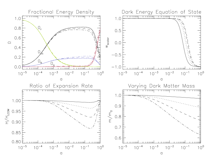
Figure 1: (Color Online) Figures to illustrate the background evolution of our coupled scalar field models. Upper Left Panel: The fractional energy densities for radiation (green), coupled dark matter (black), baryons (blue) and the scalar field (red); note that $\Omega_{\mathrm{cc}}=8\pi GC(\varphi)\rho_{\mathrm{CDM}}/3H^{2}$. Upper Right Panel: The equation of state of the scalar field, $w\equiv p_{\varphi}/\rho_{\varphi}$ in which $p_{\varphi}=\frac{1}{2}\dot{\varphi}^{2}-V(\varphi)$ and $\rho_{\varphi}=\frac{1}{2}\dot{\varphi}^{2}+V(\varphi)$. Lower Left Panel: The ratio between the Hubble expansion rate in the coupled scalar field model and that in the $\Lambda$CDM paradigm, other physical parameters such as $\rho_{\mathrm{B}},\rho_{\mathrm{RAD}},\rho_{\mathrm{CDM}}$ being held the same, as a function of the scale factor $a$. Lower Right Panel: The ”varying mass” of the dark matter particles as a function of $a$ – here $m_{0}$ is the constant bare mass of the particles and $m=e^{\gamma\varphi}m_{0}$. In all figures we have chosen $\alpha=0.1$ and the solid, dotted, dashed and dot-dashed curves represent the models with $\gamma=-0.05,-0.10,-0.15$ and $-0.20$ respectively.

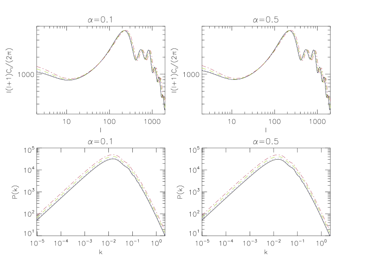
Figure 2: (Color Online) The linear power spectra of the coupled scalar field model. Upper Left Panel: The Cosmic Microwave Background (CMB) power spectra for the four models with $\alpha=0.1$. Upper Right Panel: The same but for the models with $\alpha=0.5$. Lower Left Panel: The matter power spectra at present day (redshift $z=0$) for the four models with $\alpha=0.1$. Lower Right Panel: The same but for the models with $\alpha=0.5$. In all figures the solid (black), dotted (blue), dashed (green) and dot-dashed (red) curves represent the models with $\gamma=-0.05,-0.10,-0.15$ and $-0.20$ respectively.

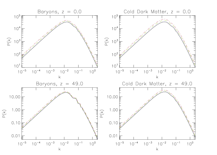
Figure 3: (Color Online) Upper Panels: The matter power spectra for baryons only (Left) and for dark matter only (Right), at current time ($z=0$). Lower Panels: The same but at an earlier time $z=49$ where the initial condition for the $N$-body simulations are computed. In all figures $\alpha=0.1$ and the solid (black), dotted (blue), dashed (green) and dot-dashed (red) curves represent the models with $\gamma=-0.05,-0.10,-0.15$ and $-0.20$ respectively.

Figure 4: Upper Left Panel: The fractional change of the growth factor $D_{+}$ of the dark matter density perturbation in the coupled scalar field model as compared with the $\Lambda$CDM prediction; for clearness shown are only the results for the two models with $\alpha=0.1,\gamma=-0.05$ and $\alpha=0.1,\gamma=-0.15$, as indicated above the curves, and for each model the solid, dotted, dashed and dot-dashed curves represent respectively the result for $k=0.0001,0.001,0.01$ and $0.1~{}\mathrm{Mpc}^{-1}$. Upper Right Panel: The same as above, but for the fractional change of $\dot{D}_{+}$ as a function of the scalar factor $a$. Lower Left Panel: The time evolution of the fractional energy density of the kinetic energy of the scalar field, $\Omega_{\mathrm{kin}}=4\pi G\dot{\varphi}^{2}/3H^{2}$ for the two models with $\alpha=0.1,\gamma=0.05$ (solid curve) and $\alpha=0.1,\gamma=-0.15$ (dotted curve) respectively. Lower Right Panel: The evolution of the density contrast of the scalar field, of which the energy density is $\rho_{\varphi}=\frac{1}{2}\dot{\varphi}^{2}+V(\varphi)$; the solid, dotted, dashed and dot-dashed curves are for four different length scales $k=0.0001,0.001,0.01$ and $0.1~{}\mathrm{Mpc}^{-1}$ respectively, and for each style of curve the upper (lower) one is for the model with $\alpha=0.1,\gamma=-0.15$ ($\alpha=0.1,\gamma=-0.05$).

III.3 Distinguishing Baryons from Dark Matter

In our simulations only dark matter particles are coupled to the scalar field. The baryons do not contribute to the scalar field equation of motion, nor are they influenced by the scalar-field fifth force. Therefore, it is important to make sure that they are distinguished and treated appropriately.

In the modified code we distinguish baryons and dark matter particles by tagging them differently. We consider the situation where 17.12% of all our matter particles are baryonic ($\Omega_{\mathrm{B}}=0.044$) and 82.88% are dark matter . During the generation of the initial condition (initial distribution and displacements of particles), we loop over all particles and for each particle we generate a random number from a uniform distribution in $[0,1]$. If this random number is less than 0.1712 then we tag the particle as baryon, otherwise we tag it as dark matter. Once these tags have been set up they are never changed again, and the code then determines whether or not a particle contributes to the scalar field evolution and feels the fifth force according to its tag.

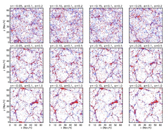
Figure 5: (Color Online) Snapshots of the particle distribution in our four coupled scalar field models as indicated by the subtitles of the panels. $a$ is the scale factor and $a=1$ is the present time. For clearness we only pick out a slice of the simulation box with $30~{}h^{-1}\mathrm{Mpc}<z<30.3~{}h^{-1}\mathrm{Mpc}$ and $0~{}h^{-1}\mathrm{Mpc}<x,y<64~{}h^{-1}\mathrm{Mpc}$. The blue dots represent dark matter particles and red dots baryons.

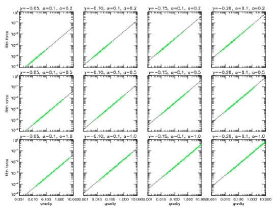
Figure 6: (Color Online) The relation between the magnitudes of the fifth force and that of gravity for the four coupled scalar field models at three different output times $a=0.2,0.5,1.0$. The black solid line in each panel represents the analytical approximation $f=2\gamma^{2}\cdot\frac{\Omega_{\mathrm{CDM}}}{\Omega_{m}}g$ (see text) and the $\sim 150,000$ green dots the results from the simulations. The particles are the same as those in Fig. 5.

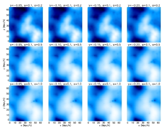
Figure 7: (Color Online) The gravitational potential on the $z$ plane where $z=32h^{-1}$ Mpc. Dark regions are where the potential is deeper while light regions are where it is shallower. The four columns are for the four models we consider and the three rows are for three output times, respectively $a=0.2,0.5$ and $1$ where $a$ is the cosmic scale factor.

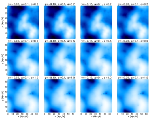
Figure 8: (Color Online) The same as Fig. 7 but for $-\varphi$ where $\varphi$ is the value of the scalar field. The negative sign is added to make the plot look similar to Fig. 7, and otherwise they will be compensating for each other.

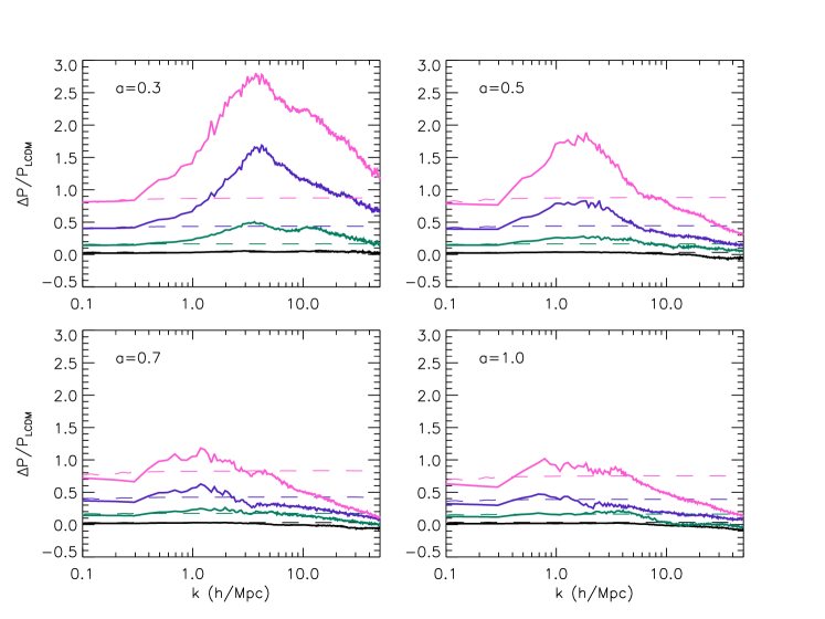
Figure 9: (Color Online) The linear and nonlinear matter power spectra $P(k)$ as compared with those of the $\Lambda$CDM paradigm. Shown are the fractional change of $P(k)$ for the four models with $\alpha=0.1$ and $\gamma=-0.05$ (black curves), $-0.10$ (green), $-0.15$ (blue), $-0.20$ (purple) and at four different output times $a=0.3$ (Upper Left Panel), $0.5$ (Upper Right), $0.7$ (Lower Left), $1.0$ (Lower Right). Solid curves are from $N$-body simulations and dashed curves from linear perturbation calculation.

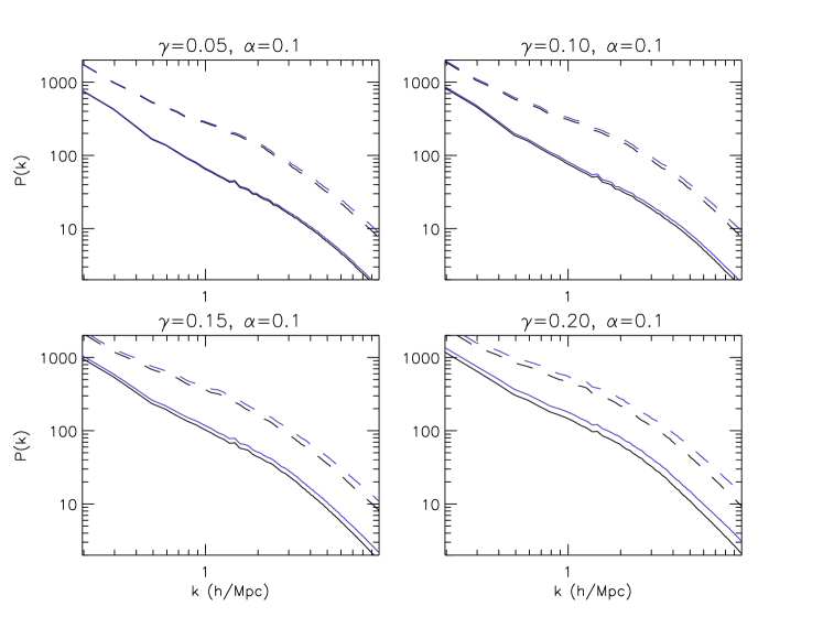
Figure 10: (Color Online) The bias between the nonlinear matter power spectra $P(k)$ of dark matter and baryons for the four models we are simulating, as indicated in the subtitles of the panels. The solid curves are for the output time $a=0.5$ and dashed curves for $a=1.0$. For each style of curve the lower (black) one is for baryons and the upper (purple) one is for dark matter.

Often in $N$-body simulations, the number of particles is chosen to be the same as the number of cells in the domain grid, but in our simulations we have set the former ($256^{3}$) to be eight times bigger than the latter ($128^{3}$). This choice obviously increases the mass resolution, but what is more important for us is that it produces a smoother and more reasonable dark matter density on the grid. In order to see this, remember that only $82.88\%$ of all particles are dark matter, which means that, if we use $128^{3}$ rather than $256^{3}$ particles, about $1/5$ of all the grid cells do not contain dark matter particles at the initial time. The resulting dark matter density therefore shows some artificial discreteness, which not only does not reflect reality but might also cause the solver for the scalar field equation to diverge. By having more particles, we can make the dark matter densities smoother and resolve the problem of over-discreteness.

III.4 Background and Linear Perturbation Evolution

In general, a coupling between the scalar field and the dark matter particles not only affects the force law and clustering properties of those particles [as described by Eqs. (II.2, 22, 28, 29, 30)], but it also influences the background and linear perturbation evolution of the Universe. The modification in the background cosmic expansion rate directly changes the rate of the matter clustering, while the modification in the linear perturbation growth might lead to a different initial condition for the $N$-body simulation from the $\Lambda$CDM result. Consequently, we must take appropriate care of these issues in the $N$-body simulations in order to obtain reliable and complete numerical results.

The background expansion rate of the universe is completely governed by (the zeroth order parts of) the scalar field equation of motion

$$\ddot{\varphi}+3H\dot{\varphi}+V_{\varphi}+C_{\varphi}\rho_{\mathrm{CDM}} = 0,$$ (40)

the Friedman equation

$$3H^{2} = \kappa\left[\rho_{\mathrm{B}}+\rho_{\mathrm{RAD}}+C(\varphi)\rho_{\mathrm{CDM}}+\frac{1}{2}\dot{\varphi}^{2}+V(\varphi)\right]\ \ \$$ (41)

where $H=\dot{a}/a$ is the Hubble expansion rate and $\rho_{\mathrm{RAD}}$ includes contributions from photons and massless neutrinos (i.e., radiation), and the Raychaudhuri equation

$$3\left(\dot{H}+H^{2}\right)$$ (42)

$$= -\frac{\kappa}{2}\left[\rho_{\mathrm{B}}+2\rho_{\mathrm{RAD}}+C(\varphi)\rho_{\mathrm{CDM}}+2\dot{\varphi}^{2}-2V(\varphi)\right].\ \ \$$

The introduction of Eq. (40) introduces a new degree of freedom $\varphi$ to the system, for which the initial condition and relevant parameter (the $\Lambda$ in $V(\varphi)$) should be chosen appropriately to guarantee consistency. More explicitly, we have to adjust the values of $\Lambda$ and $\varphi_{\mathrm{ini}},\dot{\varphi}_{\mathrm{ini}}$ so that today $H=H_{0}$ where $H_{0}$ is the measured Hubble constant which we set to be $71.9~{}\mathrm{km/s/Mpc}$ in this work. This is a nontrivial requirement and is achieved through a trial-and-error process. We shall leave all the details of the numerical algorithm to Appendix C, as they are not our major concern here.

In Fig. 1 we have shown some representative results for the influences of the scalar field coupling on the background cosmology. Clearly, for fixed $\alpha$, increasing $|\gamma|$ means increasing the coupling strength, leading to more dramatic evolution of the scalar field, and this is why in the lower right panel we can see that as $|\gamma|$ increases, so the quantity $e^{\gamma\varphi}$ falls increasingly below $1$. Meanwhile, as the scalar field rolls faster for larger $|\gamma|$, the equation of state parameter $w$ approaches $-1$ (potential-energy-dominated regime) later in time (the upper right panel). Also, because $e^{\gamma\varphi}$ deviates more from $1$, the contribution of the coupled dark matter ($\rho_{\mathrm{cc}}=\rho_{\mathrm{CDM}}e^{\gamma\varphi}$ in which $\rho_{\mathrm{CDM}}\propto a^{-3}$, see Appendix C) to the Friedmann equation [Eq. (41)] is smaller and the contributions from other matter species are greater (upper left panel). Because dark matter is the principal ingredient driving the expansion of the Universe in the matter-dominated era, this in turn implies that the expansion rate will differ from the $\Lambda$CDM prediction (lower left panel). Note that the change of expansion rate at early times necessarily cause the matter power spectrum at $z\sim 50$ to differ from the $\Lambda$CDM result, a point we will return to shortly.

In Fig. 2 we have displayed the effects of the scalar field coupling on the linear cosmic microwave background (CMB) and matter power spectra. Because of the decrease in the expansion rate, the angular diameter distance increases so that the peaks of the CMB spectrum are shifted rightwards, and on large scales the perturbation in the scalar field (cf. Fig. 4 below) modifies the integrated Sachs-Wolfe effect to increase the power at low $\ell$. The matter power spectrum, on the other hand, is increased on all scales: on large scales this is purely because the universe is now expanding more slowly, allowing matter to cluster more. On small scales there is another effect – the boost due to the scalar field fifth force, which is almost always proportional to gravity in magnitude and parallel in direction (see below). It is clear from the figure that the results are rather insensitive to the parameter $\alpha$, and so in what follows we shall only consider the case of $\alpha=0.1$.

Since we need to know the matter power spectrum at early time $z\sim 50$ in order to general initial conditions for the $N$-body simulations, we also plot it in Fig. 3. We further separate the baryons from dark matter, the latter being our major concern: on small scales it is clear that the dark matter power spectrum is greater than that of baryons, due to the extra fifth force it experiences (cf. upper panels). Most interestingly, we see that even at $z=49$ the dark matter power spectra for different models can be rather different, again due to the modified expansion rate and the fifth force. This means that in our $N$-body simulations we should not use the same initial condition (as in Li:2009sy ; Li:2010 , where the chameleon effect is so strong that at early times the matter power spectrum is indistinguishable from that of $\Lambda$CDM). Instead, we should generate initial conditions separately for different models (in our case different values for $\gamma$) – this is the topic of Sect. III.5 and Appendix A.

III.5 Initial Conditions for the $N$-Body Code

As we described in detail above, the fact that the scalar-field-dark-matter coupling begins to take effect at rather high redshift indicates that the initial conditions for the N-body simulations of our coupled scalar field models (at redshift $z_{i}\sim 50$ here) will also be different from those in $\Lambda$CDM. To account for this modification, the most straightforward approach is to generate the linear matter power spectra for our coupled scalar field models at the starting redshift $z_{i}\sim 50$, and utilize them to produce the Gaussian random density fluctuation field and displace the particles. In GRAFIC2 the matter power spectrum is generated at time $z=0$, normalized to a pre-selected value and then evolved back to $z_{i}$ and used to displace particles. We shall not follow this in our work; instead we adopt the same initial condition in CAMB at redshift $z\sim 10^{6}$ for all models including the $\Lambda$CDM one and evaluate the power spectrum at $z_{i}$ – in this way the linear $\sigma_{8}$ today will be different for different models (in contrast $\sigma_{8}$ is the same for all models in some other works). This is because we are interested in how the scalar field affects the evolution of structure as compared to $\Lambda$CDM, given the same initial condition at very early times.

In principle, the matter power spectrum at $z_{i}$ that is used in GRAFIC2 needs to be generated for each model, for example by linear perturbation code that is default in GRAFIC2; however, here we adopt a more economical method. To see this, in the upper panels of Fig. 4 we have displayed the time evolution of $\left[D_{+}-D_{+,\Lambda\mathrm{CDM}}\right]/D_{+,\Lambda\mathrm{CDM}}$ as well as $\left[\dot{D}_{+}-\dot{D}_{+,\Lambda\mathrm{CDM}}\right]/\dot{D}_{+,\Lambda\mathrm{CDM}}$, with $D_{+}$ being the linear growth factor we have discussed in Appendix D. For simplicity, we only show these for the two models with $\alpha=0.1$ and $\gamma=-0.05,-0.15$ as indicated in the figure, and for each model the solid, dotted, dashed and dash-dotted curves represent respectively the results for $k=0.0001$, $0.001$, $0.01$ and $0.1\mathrm{Mpc}^{-1}$. There are several important features in these plots. First, at early times ($z\gtrsim 10^{4}$) we see that the difference is negligible as the scalar field has yet to take effect. Second, on large scales (small $k$) the results tend to converge to a curve which describes how the change of background expansion rate modifies the density growth (the fifth force has no effect here because the scale is out of its range). Third, on smaller scales (large $k$) the fifth force begins to act and further enhances the growth of dark matter density perturbation. These plots show that $\tilde{D}_{+}$, the dark matter linear growth factor, depends on both $k$ and time as we mentioned in Appendix D, and this must be taken into account.

As detailed in Appendix D, the displacement and peculiar velocity of particles are given by $D_{+}\mathbf{d}$ and $\dot{D}_{+}\mathbf{d}$ respectively, where $\mathbf{d}$ is a vector which is the same for different models (remember again we start with the same initial condition in CAMB at $z\sim 10^{6}$). Consequently, the differences in the displacements and peculiar velocities in our models are equivalent to the differences in $D_{+}\left(z_{i}\right)$ and $\dot{D}_{+}\left(z_{i}\right)$. Instead of evaluating $D_{+}\left(z_{i}\right)$ and $\dot{D}_{+}\left(z_{i}\right)$ with (a modified version of) GRAFIC2 for each model, we use the $\Lambda$CDM results for $D_{+}\left(z_{i}\right)$ and $\dot{D}_{+}\left(z_{i}\right)$ computed by GRAFIC2, and also calculate $\mu_{1}\equiv D_{+}/D_{+,\Lambda\mathrm{CDM}}$ and $\mu_{2}\equiv\dot{D}_{+}/\dot{D}_{+,\Lambda\mathrm{CDM}}$ at $z_{i}$ using CAMB. Then the particle displacement and peculiar velocity in the coupled scalar field models are simply given respectively by $\mu_{1,2}$ times those generated by GRAFIC2.

Furthermore, we shall take into account the differences between the coupling and non-coupling matter species as following. The baryons do not feel the fifth force (remember that ’baryons’ here simply means non-coupling dark matter particles, and this is why we do not use the baryon matter power spectrum generated by CAMB to displace these particles). The difference between the baryonic linear growth factor $D_{+}$ from $D_{+,\Lambda\mathrm{CDM}}$ is mainly due to the modified expansion rate, and so we use the $D_{+}$ calculated for very small $k$ to evaluate $\mu_{1,2}$ for baryons. Dark matter particles, on the other hand, do feel the fifth force which, on small scales, has a magnitude of $2\gamma^{2}$ times that of gravity, and so we use the $\tilde{D}_{+}$ calculated for large $k$ to evaluate $\tilde{\mu}_{1,2}$ for dark matter. In this way, the bias between the two matter species is approximately reflected in our initial conditions. The scale dependence of $D_{+}$ does not appear to have been considered in generating initial conditions in the earlier literature.

When generating the initial displacement and peculiar velocities of particles, we run a random number generator for a variable with a uniform distribution $U[0,1]$. As mentioned above, if the number generated is less than $\Omega_{\mathrm{B}}/\left(\Omega_{\mathrm{B}}+\Omega_{\mathrm{CDM}}\right)$, we tag the particle as a baryon and use $\mu_{1,2}$ to displace it; otherwise we tag the particle as dark matter and use $\tilde{\mu}_{1,2}$ to compute its displacement and velocity. Once this has been done, no particle will ever be re-tagged so that the consistency is not spoiled. Those particles tagged as dark matter will contribute to the scalar field evolution and be influenced by the scalar field fifth force, while those which are tagged as baryons will not.

IV Simulation Results

In this section we present the main results from the $N$-body simulations we have performed. We start by listing some preliminary results to give a rough idea about the effects of the couplings we are studying.

IV.1 Preliminary Results

In Fig. 5 we show snapshots of the particle distribution at different output times. We can see clearly the trend of matter clustering. The blue and red dots are the dark matter and baryons particles respectively.

Since one of the most important influences of the scalar field coupling is to exert a fifth force on the dark matter particles, we are interested in the magnitude of the fifth force as compared with that of gravity. This is given in Fig. 6, where we have again displayed the results for the simulated models at different output times. To understand this figure, note that if the contributions from the scalar field potential to the Poisson equation and scalar field equation of motion are negligible (which turns out to be the case in our simulations) and if all particles (dark matter and baryons) have the same coupling to the scalar field, then the right hand sides of Eqs. (35, 36) are proportional, with a coefficient $2\gamma$, which implies that $u=2\gamma\Phi_{c}$; thus Eq. (34) says that the strengths of fifth force ($f$) and gravity ($g$) should satisfy $f=2\gamma^{2}g$.

In our models only a fraction $\Omega_{\mathrm{CDM}}/\Omega_{m}$, where $\Omega_{m}=\Omega_{\mathrm{CDM}}+\Omega_{\mathrm{B}}$, of all the particles are coupled to the scalar field. Thus, assuming dark matter and baryonic particles are distributed in the same way, we should have

$$f = 2\gamma^{2}\frac{\Omega_{\mathrm{CDM}}}{\Omega_{m}}g$$ (43)

because only a fraction $\Omega_{\mathrm{CDM}}/\Omega_{m}$ of the particles which produce gravity also produce the fifth force. Eq. (43) is plotted in Fig. 6 as the solid lines. The dots are the simulation results for $f/g$ for the particles outputted in Fig. 5. The agreement between the analytical approximation and numerical solution is remarkably good, which serves as a test of our Newton-Gauss-Seidel solver of the scalar field equation of motion .

Furthermore, Fig. 6 also shows some clearly different feature from the results of Li:2010 , in which the fifth force is suppressed by the chameleon mechanism in certain cases (such as at early times and in high-density regions). Here, the fifth force is not suppressed because the potential $V(\varphi)$ is negligible, and the approximation Eq. (43) works well anywhere all the time. This confirms our earlier claim that the matter power spectrum will be changed at early times as will be the initial condition for the $N$-body code.

As should evident now, the spatial configuration of the scalar field $\varphi$, or equivalently the rescaled scalar field $u$, should closely follow that of the gravitational potential $\Phi_{c}$, for the same reasons that led to Eq. (43). Figs. 7 and 8 confirm this: as can be seen there, for all the models and all the output times, the configurations of $-u$ and $\Phi_{c}$ are indistinguishable.

The above figures show that in our coupled scalar field models the fifth force $f$ (scalar field $u$) closely mimics the gravity $g$ (gravitational potential $\Phi_{c}$), and so the approximation $f=2\gamma^{2}g$, used in many other previous simulation works (e.g. Maccio:2004 ), is a good one.

IV.2 Matter Power Spectrum

The nonlinear matter power spectrum measured from the output particle distribution is of more observational interest and it is the theme of this subsection. The matter power spectrum in the present work is measured using POWMES powmes , which is a publicly available code based on the Taylor expansion of trigonometric functions and yields Fourier modes from a number of fast Fourier transforms controlled by the order of the expansion.

Fig. 9 displays the fractional changes of the matter power spectra $P(k)$ due to the scalar field coupling, where $\Delta P\equiv P_{\mathrm{scalar}}-P_{\Lambda\mathrm{CDM}}$. For comparison, we have also shown the linear results as dashed curves. We can see that on large scales (small $k$) there is an overall agreement between the linear and nonlinear predictions, which is not surprising since those scales have not experiences much nonlinear complication. The agreement is very good at early times (the top panels) when nonlinear effects generally have not taken place on scales $k\sim 0.1~{}h\mathrm{Mpc}^{-1}$; at late times (top curves in bottom panels) there is a slight mismatch, which is understandable because our simulation box is not big enough to allow measurement of $P(k)$ below $k=0.1~{}h\mathrm{Mpc}^{-1}$ where nonlinear effects already enter. Indeed, even in the latter case, we can see the trend that the linear and nonlinear curves merge towards at small-$k$. The fact that the nonlinear $P(k)$ reduces to the linear one on large scales is not trivial as the background cosmology in our $N$-body simulations has also been modified (as it is in CAMB, which is used for the linear calculation), and we take this as another test of our modified MLAPM code.

The main advantage of the $N$-body simulation is its ability to probe the nonlinear structure formation and so we are more concerned with the $P(k)$ on smaller scales, which is also plotted in Fig. 9. We can see that on intermediate scales ($k\sim 1~{}h\mathrm{Mpc}^{-1}$) the nonlinear $P(k)$ beats the linear one, but on even smaller scales it falls behind the linear value again. For the four models in our simulations the enhancements of the matter power range from negligible to $\sim 100\%$, but much of the enhancement is due to the modified background expansion and is already seen in the linear results. More interestingly, the enhancement is more significant at earlier times. This can been understood as follows: at later times the contribution of the dark matter density to the Poisson equation (and thus the gravitational potential) is decreased due to the coupling function $C(\varphi)$ becoming increasingly less than 1, weakening further clustering of the (not only dark but also baryonic) matter. Note that such a trend can also be seen in the linear $P(k)$, by comparing the bottom panels, although it is not so obvious.

In order to display the bias developed between baryons and dark matter, we have also plotted the $P(k)$ for baryons and dark matter separately in Fig. 10. As expected, the $P(k)$ for dark matter is always larger, signifying a stronger clustering due to the assistance from the fifth force. The larger $|\gamma|$ is, the stronger the fifth force will be, and the larger the bias will become.

IV.3 Mass Function

We identify halos in our $N$-body simulations using MHF (MLAPM Halo Finder) mhf , which is the default halo finder for MLAPM. MHF optimally utilizes the refinement structure of the simulation grids to pin down the regions where potential halos reside and organize the refinement hierarchy into a tree structure. MLAPM refines grids according to the particle density on them and so the boundaries of the refinements are simply isodensity contours. MHF collects the particles within these isodensity contours (as well as some particles outside). It then performs the following operations: (i) assuming spherical symmetry of the halo, calculate the escape velocity $v_{esc}$ at the position of each particle, (ii) if the velocity of the particle exceeds $v_{esc}$ then it does not belong to the virialized halo and is removed. Steps (i) and (ii) are then iterated until all unbound particles are removed from the halo or the number of particles in the halo falls below a pre-defined threshold, which is 20 in our simulations. Note that the removal of unbound particles is not used in some halo finders using the spherical overdensity (SO) algorithm, which includes the particles in the halo as long as they are within the radius of a virial density contrast. Another advantage of MHF is that it does not require a pre-defined linking length in finding halos, such as the friend-of-friend procedure.

As explained in detail in Li:2010 , part of the MHF algorithm also needs to be modified for the coupled scalar field model, because the scalar field $\varphi$ behaves as an extra ”potential” (which produces the fifth force) and so the dark matter particles experience a deeper total ”gravitational” potential than in the $\Lambda$CDM paradigm, all other things being equal. Consequently, the escape velocity for dark matter particles increases compared with the Newtonian prediction. As the dark matter particles in the coupled scalar field simulations are typically faster than in the $\Lambda$CDM simulation, if we underestimate $v_{esc}$ then some particles which should have remained in the halo will be incorrectly removed by MHF. In Li:2010 it was found that the underestimate of the mass function by using default MHF in the coupled scalar field models could be up to a few percent.

In the models we are considering here, things are even more complicated. In Li:2010 , the chameleon mechanism ensures that the scalar field takes a very tiny value everywhere, all the time (typically $\sqrt{\kappa}\varphi\lesssim 10^{-5}$) and so the coupling function $C(\varphi)=e^{\gamma\sqrt{\kappa}\varphi}\doteq 1$ is a very good approximation – this means that the contribution of the dark matter to the Poisson equation is not significantly modified compared with that in $\Lambda$CDM. In the models here, however, $C(\varphi)$ can be up to $30\%$ less than $1$, so that the source term of the Poisson equation is significantly different from $\Lambda$CDM.

Obviously, we need to take both of these two major changes into account when we design a new algorithm to identify halos. An exact analytical calculation of the escape velocity and Poisson source term in the coupled scalar field model turns out be difficult, and so we introduce an approximate alternative, which is based on the MHF default method ahf .

The default MHF code works out $v_{esc}$ using the Newtonian result

$$v^{2}_{esc} = 2|\Phi|,$$ (44)

in which $\Phi$ is the gravitational potential. Under the assumption of spherical symmetry for the halos, the Poisson equation $\nabla^{2}\Phi=4\pi G\rho_{m}$ could be integrated once to give

$$\frac{d\Phi}{dr} = \frac{GM(<r)}{r^{2}}$$ (45)

which is just the Newtonian force law. This equation can be integrated once again to obtain

$$\Phi(r) = G\int^{r}_{0}\frac{M(<r^{\prime})}{r^{\prime 2}}dr^{\prime}+\Phi_{0}$$ (46)

where $\Phi_{0}$ is an integration constant and can be fixed ahf by requiring that $\Phi(r=\infty)=0$ as

$$\Phi_{0} = \frac{GM_{vir}}{R_{vir}}+G\int^{R_{vir}}_{0}\frac{M(<r^{\prime})}{r^{\prime 2}}dr^{\prime},$$ (47)

in which $R_{vir}$ is the virial radius of the halo and $M_{vir}$ is the mass enclosed in $R_{vir}$.

In the coupled scalar field models here, the two modifications mentioned above are reflected in Eqs. (44, 45).

Figure 11: The mass functions at $a=1$ for the four coupled scalar field models under investigation, as indicated by the subtitles of the panels. The dashed curves are the corresponding result of $\Lambda$CDM.

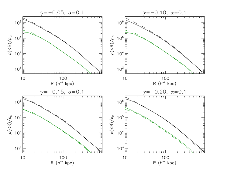
Figure 12: (Color Online) The internal density profiled of two selected halos (see text) at $a=1$. The four panels are for the four models we have simulated, as illustrated by the subtitles. In all panels solid curves are for the coupled scalar field model and dashed curves for $\Lambda$CDM. The upper (black) curves are result for halo I and lower (green) curves for halo II.

Figure 13: The fractional change of the internal density profile due to the dark matter being coupled to the scalar field, $[\rho(<R)-\rho_{\Lambda\mathrm{CDM}}(<R)]/\rho_{\Lambda\mathrm{CDM}}(<R)$. The solid curves are the average of ten of the heaviest halos in our simulation boxes and the dashed curve is 0. We show this for the four models we have simulated, as illustrated by the subtitles.

Figure 14: The internal density profiles for dark matter (solid curves) and baryons (dashed curves) separately. We show this for the four models we have simulated, as indicated by the subtitles. In each panel the upper two curves are for halo I and the lower two curves for halo II.

For Eq. (44), we realize that the gravitational potential $\Phi$ is not the only factor determining the escape velocity: there is also a contribution from the scalar field $\varphi$. There are different ways to approach this problem, the simplest of which is to obtain the total ”potential” by rescaling $\Phi$ with a constant (remember we have shown in Sect. IV.1 that $\varphi\propto\Phi$ is a good approximation all the time and everywhere). A more delicate approach can be devised by noting that in the default MHF code, Eq. (45) is used in the numerical integrations to obtain both $\Phi(r)$ and $\Phi_{0}$ [cf. Eqs.(46, 47)]. More explicitly, the code loops over all particles in the halo in ascending order of the distance from the halo centre, and whenever a particle is encountered its mass is uniformly distributed into the spherical shell between the particle and its previous particle (the thickness of the shell is now the $dr$ of the integration). When the fifth force is added, we call its contribution to the total ”gravitational” potential $\Phi_{\varphi}$ and its value at infinity, $\Phi_{\varphi 0}$. Our estimate of the escape velocity is now, instead of Eq. (44), given by

$$v_{esc}^{2}=2|\Phi+\Phi_{\varphi}-\Phi_{0}-\Phi_{\varphi 0}|.$$ (48)

We have recorded the components of gravity and the fifth force for each particle in the simulation, and so the ratio $f/g$ can be computed at the position of each particle, which gives $\left(\Phi_{\varphi}-\Phi_{\varphi 0}\right)/\left(\Phi-\Phi_{0}\right)$ at that position, which can be used in Eq. (48). In this way we have, at least approximately, taken into account the fifth force and $\Phi_{\varphi}$.

For Eq. (45), which is used to compute $\Phi$ and $\Phi_{0}$, we know that it is applicable in the coupled scalar field model as well, because the contribution from the scalar field potential is negligible. But one should be careful when interpreting the mass $M$ here: it is not the total bare mass of all the particles ($M_{\mathrm{B}}+M_{\mathrm{CDM}}$) within radius $r$, but $M_{\mathrm{B}}+C(\varphi)M_{\mathrm{CDM}}$. Such a fact can be taken into account by multiplying the mass of each dark matter (not baryonic) particle by $C(\varphi),$ which is evaluated using the $\varphi$ at the position of that particle (which we have recorded too). Note that observations of the masses are made by registering gravitational effect, and so the halo mass we measure should be $M_{\mathrm{B}}+C(\varphi)M_{\mathrm{CDM}}$ rather than $M_{\mathrm{B}}+M_{\mathrm{CDM}}$: in what follows we will always talk about the former unless otherwise stated.

In Fig. 11 we have plotted the mass functions of our four coupled scalar field models at the current time, as compared with the prediction of the $\Lambda$CDM paradigm. Obviously, as the coupling between dark matter and the scalar field becomes stronger, more heavy halos will be produced during structure formation. However, it is not yet clear which physical effect is mainly responsible for such a pattern, and several factors could be crucial. For examples, as $|\gamma|$ increases, the fifth force strengthens and the background expansion gets slower, both of which would help boost the clustering of matter; on the other hand, the dark matter’s contribution to the Poisson equation is weakened due to $C(\varphi)$ becoming increasingly less than $1$ – this will weaken the clustering of matter. Detailed study of the significance of these different physical effects is beyond the scope of this work.

IV.4 Halo Properties

Finally, we are also interested in the properties of the dark matter halos in the coupled scalar field models. In the case of a chameleon-like scalar field, ref Li:2010 shows that there is a strong environmental dependence on density profile and baryon-dark-matter bias inside the halo, which is controlled by the model parameters in a complicated way. In the models generated here, the fifth force is everywhere unsuppressed and we do not expect such an environmental dependence as seen in Li:2010 . However, we have several factors mentioned in Sect. IV.3, which can potentially lead to interesting new features.

We will look first at the internal density profiles, which can be measured down to small radii thanks to the higher spatial resolution of the self-refinement code. We have selected two typical halos from each simulation. Halo I is centred on $(x,y,z)\sim(32.4,31.5,61.2)h^{-1}$ Mpc, which is slightly different for different simulations, and has a virial mass $M_{vir}\sim 1.29\times 10^{14}h^{-1}~{}M_{\bigodot}$; halo II is centred on $(x,y,z)\sim(54.8,39.8,35.7)h^{-1}$ Mpc, which is also slightly different for different simulations, and has a virial mass $M_{vir}\sim 1.90\times 10^{13}h^{-1}~{}M_{\bigodot}$ (note here that the virial masses are for the $\Lambda$CDM simulations; for scalar-field simulations they can be, and generally are, larger).

Fig. 12 summarizes what we have, and it shows that the density profile for the coupled scalar field model is rather similar to that of $\Lambda$CDM, except that for the innermost part the overdensity for the scalar field model (solid curves) drops below that of $\Lambda$CDM (dashed curves). Such a phenomenon has previously been detected by the authors of Baldi:2008 and explained as mainly due to the velocity-dependent acceleration of dark matter particles [the last term in Eq. (26)]. However, here we find here that such a trend does not continue with increasing $|\gamma|$ and is indeed reversed for large $|\gamma|$ values. To see this more explicitly, in Fig. 13 we have shown the quantity $\Delta\rho(<R)/\rho_{\Lambda\mathrm{CDM}}(<R)$ (where $\rho(<R)$ is the average density inside radius $R$ and $\Delta$ means the difference between the coupled scalar field model and $\Lambda$CDM) averaged over 10 of the heaviest halos of our simulations. This shows clearly that for small $|\gamma|$ values the inner density is systematically lower in our coupled scalar field models than in $\Lambda$CDM while this is not necessarily true for the density in the outer part of the halos. Also, as $|\gamma|$ increases, the lowering of inner density becomes less significant, and finally for $\gamma=-0.20$ we see the opposite trend emerge. The physical explanations of the observed patterns are not of prime interest to our study here.

Next, we can look at the bias between baryons and dark matter in the halos, which is displayed in Fig. 14. As expected, we find that the dark matter density is constantly higher than that of baryons, due to the extra force they feel (note that other factors, such as the cosmic expansion rate and the modification of the source term in the Poisson equation, have the same influence on dark matter and baryons). In general, the bias increases with the coupling strength $|\gamma|$ which is easy to understand.

V Summary and Discussion

Couplings between any scalar field and (some of) the matter species can affect cosmology in various ways. There are two principal effects: modified source terms in the gravitational field equations (channel I) and direct new interactions between particles of the coupled matter species (channel II).

The effects through channel II arise in an inhomogeneous universe, but not in background cosmology. In principle, there is only effect of this sort – the fifth force, due to the exchanges of scalar quanta between matter particles. In practice, (e.g., in $N$-body simulations), the scalar field $\varphi$ is computed in the fundamental observer’s frame while the fifth force must be evaluated in individual particle frames; consequently, the fifth force is split into two parts: the part from the spatial gradient of the scalar field $\delta\varphi$ in the fundamental observer’s frame (which is independent of the particle’s peculiar velocity $v$) and the part due to frame transformation which is proportional to $v$. In a homogeneous universe, there is no spatial gradient and all matter particles are comoving with the fundamental observers, so $v=0$, and therefore the channel II effects vanish. In an inhomogeneous universe both terms are nonzero in general, leading to a net force which strengthens the attraction between particles, and enhances their gravitational clustering.

The effects arising through channel I appear both in homogeneous (via the Friedmann and Raychaudhuri equations) and inhomogeneous (via the Poisson equation) universes. They arise mainly via a renormalization of the contributions to the total density from the coupled matter species and by a new contribution from the scalar field itself.  The exact effects depend on the specific forms of the scalar potential and coupling function. Here, we list our main findings for an inverse power-law potential Eq. (13), with an exponential coupling Eq. (14), and the model parameters given in Sect. III.2.

For the background cosmology, the contribution to the Friedmann equation from dark matter is renormalized by $C(\varphi)<1$, and $C(\varphi)$ decreases as the coupling constant $|\gamma|$ increases. As a result, a stronger coupling (larger $|\gamma|$) produces lower cosmic expansion rate during the matter-dominated era (Fig. 1) , which will in turn helps enhance the clustering of matter and promotes structure formation.

Such an enhancement is just what we have observed from our linear perturbation analysis (Figs. 2 and 3): on very large scales, which are beyond the range of the fifth force effects, the matter power spectrum increases with $|\gamma|$. On small scales, the fifth force helps to enhance the matter power, making it increase further than predicted in $\Lambda$CDM (comparing the left to the right panels of Fig. 3, where we have separated baryons, which have no scalar coupling, from dark matter, which has). This enhancement starts at a rather early, and so the scalar field does leave imprints on the matter power spectrum at $z\sim 50$, which means that the initial condition for $N$-body simulations also needs to modified. For example, in the model with $|\gamma|=0.15$, we have found that :

(i) The density perturbation at $z\sim 49$ is about $10\%$ larger than the corresponding result in $\Lambda$CDM for baryons (due to slower cosmic expansion) and about $12\%$ larger for dark matter (due to the slower expansion and the fifth force effects);

(ii) The average velocity at the same time is about $8\%$ larger than the corresponding result in $\Lambda$CDM for baryons and about $10\%$ larger for dark matter. We introduce a quick method to take these changes into account when generating initial conditions for $N$-body simulations.

One of the most important results from our $N$-body simulations is the magnitude of fifth force. Fig. 6 shows that everywhere and at any time (i.e., in both high and low density regions) the fifth force (or more precisely, the velocity-independent part of it) is proportional to gravity in magnitude (with a coefficient $2\gamma^{2}$ when only considering dark matter). This is the approximation used in many previous simplified simulations, and our results confirm numerically that this approximation works fairly well, at least for those cases where the scalar potential is unimportant, such as ours. We emphasize, however, that the velocity-dependent part of the fifth force should not be dropped (as in some previous simulations) unless there is good reason to do so (see Li:2010 ).

For the nonlinear matter power spectrum (Fig. 9), we find that the $N$-body simulations show agreement with linear perturbation analysis on large scales. On intermediate scales, our simulations predict significant enhancement in the matter power over that predicted both by linear perturbation analysis and by the $\Lambda$CDM paradigm. This enhancement is strongest at early epochs but gradually weakens at late times. One possible reason for this is that the scalar coupling, $C(\varphi),$ decreases with time, and reduces the contribution of dark matter to the gravitational potential, so weakening further clustering, but this still needs to be investigated in more detail.

The bias between dark matter and baryons increases with time and with coupling strength $|\gamma|$. This is because larger $|\gamma|$ implies stronger fifth forces and therefore stronger total forces act on dark matter particles compared to baryons. As time passes, the bias has more time to develop and so increases as well (Fig. 10). Using the same reasoning, the fifth force increases the attraction of dark matter particles and so heavier halos are expected to form during the structure formation (Fig. 11). In order to identify gravitationally bound and virialized halos in our models we must also take into account this scalar coupling (Sect. IV.4).

The scalar field coupling also has impacts on the internal density profiles of the halos (Figs. 12 and 13). We average ten of the heaviest halos and find that

(i) When compared with $\Lambda$CDM, the overdensities in the inner regions can be lower while those in the outer regions is higher, showing the failure of the halos to retain particles in the inner region, either because the particles move too fast or because the attractive potential at the centre is too weak;

(ii) The suppression of inner density compared with $\Lambda$CDM weakens, rather than strengthens, as $|\gamma|$ increases. Indeed, for $|\gamma|=0.2$ the density is higher than $\Lambda$CDM result throughout the halos. More detailed studies are needed to clarify the leading effect responsible for this observed pattern.

(iii) There is a bias between density profiles for baryons and dark matter (Fig. 14): the dark matter density is always higher because it experiences the fifth force which boosts its clustering.

In summary, in this paper we have been given a comprehensive description of the methodology and implementation of general $N$-body simulations for coupled scalar field models. Some important issues in these simulations have been addressed here for the first time: the consistent solution of the scalar field and fifth force, the fifth force effects on generating initial conditions, and the effects of scalar field on identifying virialized halos. Although the situation is complex, we have identified interesting new features in these models. We hope these developments will lead to more detailed study of nonlinear structure formation in this class of models and facilitate their subsequent confrontation with observational data.

Appendix A Discretized Equations for the $N$-body Simulations

In the MLAPM code for Poisson equation Eq. (35) is (and in our modified code the scalar field equation of motion Eq. (36) will also be) solved on discretized grid points, so we must develop the discrete versions of Eqs. (33 - 36) to be implemented in the code. First, we write down the full formalism of the relevant equations.

Introducing the variable $u$ (cf. Sect. II.3), the Poisson equation becomes

$$\nabla^{2}\Phi_{c}$$ (49)

$$= \frac{3}{2}\Omega_{\mathrm{CDM}}\left\{\rho_{c,\mathrm{CDM}}\exp\left[\gamma\left(\sqrt{\kappa}\bar{\varphi}+\frac{B^{2}H^{2}_{0}}{ac^{2}}u\right)\right]-e^{\gamma\sqrt{\kappa}\bar{\varphi}}\right\}$$

$$+\frac{3}{2}\Omega_{\mathrm{B}}\left(\rho_{c,\mathrm{B}}-1\right)-\frac{3\lambda a^{3}}{\left[\sqrt{\kappa}\bar{\varphi}+\frac{B^{2}H^{2}_{0}}{ac^{2}}u\right]^{\alpha}}+\frac{3\lambda a^{3}}{\left[\sqrt{\kappa}\bar{\varphi}\right]^{\alpha}},\ \ \ \ \$$

where $\lambda$ is defined in Eq. (20) and is a constant of $O(1)$ (actually $\lambda\sim\Omega_{\mathrm{DE}}$ where _DE means dark energy). Its value and that of the quantity $\sqrt{\kappa}\bar{\varphi}$ are determined solely by the background evolution. The computation of the background quantities is discussed in Sect. III.4.

The scalar field equation of motion now becomes

$$\nabla^{2}u = 3\gamma\Omega_{\mathrm{CDM}}\rho_{c,\mathrm{CDM}}\exp\left[\gamma\left(\sqrt{\kappa}\bar{\varphi}+\frac{B^{2}H^{2}_{0}}{ac^{2}}u\right)\right]$$ (50)

$$-\frac{3\alpha\lambda a^{3}}{\left[\sqrt{\kappa}\bar{\varphi}+\frac{B^{2}H^{2}_{0}}{ac^{2}}u\right]^{1+\alpha}}-3\gamma\Omega_{\mathrm{CDM}}e^{\gamma\sqrt{\kappa}\bar{\varphi}}$$

$$+\frac{3\alpha\lambda a^{3}}{\left[\sqrt{\kappa}\bar{\varphi}\right]^{1+\alpha}}.$$

So, in terms of the new variable $u$, the set of equations used in the $N$-body code is Eqs. (33, 34) plus Eqs. (49, 50). These equations were used in the code. Among them, Eqs. (49, 34) will use the value of $u,$ while Eq. (50) solves for $u$. In order that these equations can be integrated into MLAPM, we need to discretize Eq. (50) for the application of Newton-Gauss-Seidel relaxation method. This involves writing down a discrete version of this equation on a uniform grid with grid spacing $h$. Suppose we want to achieve second-order precision, as is in the default Poisson solver of MLAPM, then $\nabla^{2}u$ in one dimension can be written as

$$\nabla^{2}u \rightarrow \nabla^{h2}u_{j}\ =\ \frac{u_{j+1}+u_{j-1}-2u_{j}}{h^{2}}$$ (51)

where a subscript _j means that the quantity is evaluated on the $j$-th point. The generalization to three dimensions is straightforward.

The discrete version of Eq. (50) is

$$L^{h}\left(u_{i,j,k}\right) = 0,$$ (52)

in which

$$L^{h}\left(u_{i,j,k}\right) = \frac{1}{h^{2}}\left[u_{i+1,j,k}+u_{i-1,j,k}+u_{i,j+1,k}+u_{i,j-1,k}+u_{i,j,k+1}+u_{i,j,k-1}-6u_{i,j,k}\right]$$ (53)

$$-\left[3\gamma\Omega_{\mathrm{CDM}}\rho_{c,\mathrm{CDM}}\exp\left[\gamma\left(\sqrt{\kappa}\bar{\varphi}+\frac{B^{2}H^{2}_{0}}{ac^{2}}u_{i,j,k}\right)\right]-\frac{3\alpha\lambda a^{3}}{\left[\sqrt{\kappa}\bar{\varphi}+\frac{B^{2}H^{2}_{0}}{ac^{2}}u_{i,j,k}\right]^{1+\alpha}}\right]$$

$$+\left[3\gamma\Omega_{\mathrm{CDM}}e^{\gamma\sqrt{\kappa}\bar{\varphi}}-\frac{3\alpha\lambda a^{3}}{\left[\sqrt{\kappa}\bar{\varphi}\right]^{1+\alpha}}\right].$$

Then, the Newton-Gauss-Seidel iteration says that we can obtain a new (and often more accurate) solution of $u$, $u_{i,j,k}^{\mathrm{new}}$, using our knowledge about the old (and less accurate) solution $u_{i,j,k}^{\mathrm{old}}$ via

$$u^{\mathrm{new}}_{i,j,k} = u^{\mathrm{old}}_{i,j,k}-\frac{L^{h}\left(u^{\mathrm{old}}_{i,j,k}\right)}{\partial L^{h}\left(u^{\mathrm{old}}_{i,j,k}\right)/\partial u_{i,j,k}}.$$ (54)

The old solution will be replaced by the new solution to $u_{i,j,k}$ once the new solution is ready, using the red-black Gauss-Seidel sweeping scheme. Note that

$$\frac{\partial L^{h}(u_{i,j,k})}{\partial u_{i,j,k}} = -\frac{6}{h^{2}}-3\gamma^{2}\frac{\left(H_{0}B\right)^{2}}{ac^{2}}\Omega_{\mathrm{CDM}}\rho^{\mathrm{CDM}}_{c,i,j,k}\exp\left[\gamma\left(\sqrt{\kappa}\bar{\varphi}+\frac{B^{2}H^{2}_{0}}{ac^{2}}u_{i,j,k}\right)\right]-\frac{\left(H_{0}B\right)^{2}}{ac^{2}}\frac{3\alpha(1+\alpha)\lambda a^{3}}{\left[\sqrt{\kappa}\bar{\varphi}+\frac{B^{2}H^{2}_{0}}{ac^{2}}u_{i,j,k}\right]^{2+\alpha}}.\ \ \$$ (55)

In principle, if we start from a high redshift, then the initial guess of $u_{i,j,k}$ for the relaxation could be so chosen that the initial value of $\varphi$ in all space is equal to the background value $\bar{\varphi}$, because at this time we expect this to be approximately true any way. At subsequent time-steps we could use the solution for $u_{i,j,k}$ from the previous time-step as our initial guess. If the timestep is small enough then we would expect $u$ to change only slightly between consecutive timesteps so that such a guess will be good enough for the iterations to converge quickly.

In practice, however, due to specific features and the algorithm of the MLAPM code Knebe:2001 , the above procedure may be slightly different in details.

Appendix B The Dark Matter Lagrangian

For simplicity let us write the CDM Lagrangian as $\mathcal{L}_{\mathrm{CDM}}=F^{1/2}=\sqrt{g_{ab}\dot{x}^{a}\dot{x}^{b}}$ (i.e., neglecting the mass term and $\delta$-function term in Eq. (2)) in which $\dot{x}^{a}\equiv dx^{a}/ds$ and $s$ is some general parameterization of a particle’s geodesic (we only use this definition in this appendix and note that in other places in the paper $\dot{x}$ has different meaning). The Euler-Lagrange equation is

$$\frac{d}{ds}\frac{\partial\mathcal{L}\mathrm{CDM}}{\partial\dot{x}^{a}} = \frac{\partial\mathcal{L}_{\mathrm{CDM}}}{\partial x^{a}}$$ (56)

in which we have

$$\frac{\partial\mathcal{L}_{\mathrm{CDM}}}{\partial x^{a}} = \frac{1}{2}F^{-1/2}g_{bc,a}\dot{x}^{b}\dot{x}^{c},$$

$$\frac{\partial\mathcal{L}_{\mathrm{CDM}}}{\partial\dot{x}^{a}} = \frac{1}{2}F^{-1/2}\frac{\partial}{\partial\dot{x}^{a}}(g_{bc}\dot{x}^{b}\dot{x}^{c})$$

$$= \frac{1}{2}F^{-1/2}g_{bc}(\delta^{b}_{a}\dot{x}^{c}+\delta^{c}_{a}\dot{x}^{b}),$$

and

$$\frac{d}{ds}\frac{\partial\mathcal{L}_{\mathrm{CDM}}}{\partial\dot{x}^{a}}$$

$$= F^{-1/2}\left[g_{ab}\ddot{x}^{b}-\frac{1}{2}F^{-1}\dot{F}g_{ab}\dot{x}^{b}+\frac{1}{2}(g_{ac,b}\dot{x}^{b}\dot{x}^{c}+g_{ab,c}\dot{x}^{b}\dot{x}^{c})\right]$$

so that the Lagrange equation becomes

$$\ddot{x}^{d}-\frac{1}{2}F^{-1}\dot{F}\dot{x}^{d}+\Gamma^{d}_{bc}\dot{x}^{b}\dot{x}^{c} = 0.$$ (57)

For timelike geodesics we can choose $s=\tau$ ($\tau$ being the proper time) which means that $F=1$ so that Eq. (57) becomes the usual geodesic equation

$$\ddot{x}^{a}+\Gamma^{a}_{bc}\dot{x}^{b}\dot{x}^{c} = 0.$$ (58)

If $F\neq 1,$ then we need to retain Eq. (57) as the geodesic equation, which is unfamiliar. We note that $F=1$ (and $\mathcal{L}_{\mathrm{CDM}}=1$ above) corresponds to the result in our Eq. (4). As it stands, Eq. (4) is exact. Since we use proper time $\tau$ for $s$, the geodesic equation is also written in terms of $\tau$, which means that when we switch from $\tau$ to the physical time $t$ in Eq. (23) there will be some approximation, but Eq. (23) is approximate in any case.

Appendix C An Algorithm to Solve for the Background Evolution

Here, we aim to give the formulae and an algorithm for the background field equations which can also be applied to linear Boltzmann codes such as CAMB. Throughout this Appendix we use the conformal time $\tau$ instead of the physical time $t$, and ${}^{\prime}\equiv d/d\tau,\mathcal{H}\equiv a^{\prime}/a$. All quantities appearing here are background ones unless stated otherwise.

For convenience, we will work with dimensionless quantities and define $\tilde{\varphi}\equiv\sqrt{\kappa}\varphi$ and $N\equiv\ln a$ so that

$$\tilde{\varphi}^{\prime} = \mathcal{H}\frac{d\tilde{\varphi}}{dN},$$ (59)

$$\tilde{\varphi}^{\prime\prime} = \mathcal{H}^{2}\frac{d^{2}\tilde{\varphi}}{dN^{2}}+\mathcal{H}^{\prime}\frac{d\tilde{\varphi}}{dN}.$$ (60)

With these definitions it is straightforward to show that Eq. (40) can be expressed as

$$\left(\frac{\mathcal{H}}{\mathcal{H}_{0}}\right)^{2}\frac{d^{2}\tilde{\varphi}}{dN^{2}}+\left(2\frac{\mathcal{H}^{2}}{\mathcal{H}_{0}^{2}}+\frac{\mathcal{H}^{\prime}}{\mathcal{H}_{0}^{2}}\right)\frac{d\tilde{\varphi}}{dN}$$

$$-3\alpha\lambda a^{2}\frac{1}{\tilde{\varphi}^{1+\alpha}}+\frac{3}{a}\gamma\Omega_{\mathrm{CDM}}e^{\gamma\tilde{\varphi}} = 0,$$ (61)

where $\mathcal{H}_{0}$ is the current value of $\mathcal{H}$, and the coefficients of the derivative terms are given by Eqs. (41, 42) as

$$\left(\frac{\mathcal{H}}{\mathcal{H}_{0}}\right)^{2}$$ (62)

$$= \frac{\Omega_{\mathrm{RAD}}a^{-2}+\Omega_{\mathrm{B}}a^{-1}+e^{\gamma\tilde{\varphi}}\Omega_{\mathrm{CDM}}a^{-1}+\frac{\lambda a^{2}}{\tilde{\varphi}^{\alpha}}}{1-\frac{1}{6}\left(\frac{d\tilde{\varphi}}{dN}\right)^{2}},\ \$$

and

$$\frac{\mathcal{H}^{\prime}}{\mathcal{H}^{2}_{0}} = -\frac{1}{3}\left(\frac{d\tilde{\varphi}}{dN}\right)^{2}\frac{\mathcal{H}^{2}}{\mathcal{H}_{0}^{2}}+\frac{\lambda a^{2}}{\tilde{\varphi}^{\alpha}}$$ (63)

$$-\left[\Omega_{\mathrm{RAD}}a^{-2}+\frac{1}{2}\Omega_{\mathrm{B}}a^{-1}+\frac{1}{2}e^{\gamma\tilde{\varphi}}\Omega_{\mathrm{CDM}}a^{-1}\right].\ \ \$$

In all of the above equations we have used the facts that

$$\rho_{\mathrm{CDM}} \propto a^{-3},$$

$$\rho_{\mathrm{B}} \propto a^{-3},$$

$$\rho_{\mathrm{RAD}} \propto a^{-4}.$$

We stress again that although coupled to the scalar field, the background dark-matter energy density follows the same conservation law as in $\Lambda$CDM. The effect of the coupling is reflected in the fact that there is a coefficient $e^{\gamma\tilde{\varphi}}$ in front of $\Omega_{\mathrm{CDM}}$ whenever the latter appears in the gravitational equations or the scalar field evolution equation Li:2009sy .

When solving for $\varphi$ (or $\tilde{\varphi}$), we just use Eq. (C) aided by Eqs. (62, 63). It may appear then that, given any initial values for $\tilde{\varphi}_{\mathrm{ini}}$ and $\left(d\tilde{\varphi}/dN\right)_{\mathrm{ini}},$ the evolution of $\varphi$ is obtainable. However, Eq. (62) is not necessarily satisfied for $\tilde{\varphi}$ evolved in such way. Instead, it constrains the initial condition $\tilde{\varphi}$ must start with, and the way it must subsequently evolve. This in turn is determined by the parameters $\lambda,\alpha,\gamma$; since $\alpha,\gamma$ specify a model and are fixed once the model is chosen, the only concern is $\lambda$.

For the initial conditions $\tilde{\varphi}_{\mathrm{ini}}$ and $\left(d\tilde{\varphi}/dN\right)_{\mathrm{ini}}$, we have found that the subsequent evolution of $\tilde{\varphi}$ is rather insensitive to them. Thus, we choose $\tilde{\varphi}_{\mathrm{ini}}=\left(d\tilde{\varphi}/dN\right)_{\mathrm{ini}}=0$ at some very early time (say $N_{\mathrm{ini}}$ corresponds to $a_{\mathrm{ini}}=e^{N_{\mathrm{ini}}}=10^{-6}$) in all the models. Such a choice is clearly not only practical but also reasonable, given the fact that we expect that the scalar field starts high up the potential and rolls down subsequently.

As for $\lambda$, we use a trial-and-error method to find its value which ensures that (here a subscript ₀ denotes the present-day value)

$$\Omega_{\mathrm{RAD}}+\Omega_{\mathrm{B}}+e^{\gamma\tilde{\varphi}_{0}}\Omega_{\mathrm{CDM}}+\frac{\lambda}{\tilde{\varphi}_{0}^{\alpha}} = 1-\frac{1}{6}\left(\frac{d\tilde{\varphi}}{dN}\right)^{2}_{0}$$

which comes from setting $a=1$ in Eq. (62).

We determine the correct value of $\lambda$ for any given $\alpha,\gamma$ in this way using MAPLE, and then compute the values of $\tilde{\varphi}$ and $d\tilde{\varphi}/dN$ for predefined values of $N$ stored in an array. Their values at any time are then obtained using interpolation, and with these it is straightforward to compute other relevant quantities, such as $\mathcal{H},\mathcal{H}^{\prime},$and $\varphi,$ which are used in the Boltzmann and $N$-body codes.

Appendix D The Zeldovich Approximation

The initial conditions for $N$-body simulations are conventionally generated using the Zeldovich approximation Zeldovich ; Efstathiou:1985 , which in its original form works only for non-coupled dark matter. When there is a non-minimal coupling between dark matter particles and a scalar field, it must be generalized, and we discuss this here.

Consider a particle whose actual position $\mathbf{r}$ is given as

$$\mathbf{r} = a(t)\mathbf{q}+b(t)\mathbf{d}$$ (64)

where $\mathbf{q}$ is the Lagrangian coordinate (i.e. initial comoving coordinate with displacement), $\mathbf{d}$ is the displacement from $\mathbf{q}$ and $b(t)$ governs how the displacement increases in time (or, equivalently, how the density perturbation grows). From this, we have a deformation tensor

$$\mathcal{D}_{ij} = \frac{\partial r_{i}}{\partial q_{j}}\ =\ a(t)\delta_{ij}+b(t)\frac{\partial d_{i}}{\partial q_{j}},$$ (65)

which is just the Jacobian of the coordinate transformation, providing information about the change of the size of a given volume element (centred on the particle). When the deformation is small, as in the case of the early times when we set up the initial condition, we have

$$\det\mathcal{D} \doteq a^{3}(t)\left[1+\frac{b}{a}\nabla_{\mathbf{q}}\cdot\mathbf{d}\right]$$ (66)

where we have neglected higher-order terms in $\mathbf{d,}$ and $\nabla_{\mathbf{q}}$ is the spatial derivative with respect to the Lagrangian coordinate $\mathbf{q}$. Note that the term in brackets is the fractional change of the volume element due to the collapse of matter.

In a given volume element, because we have two matter species now and their density contrasts grow at different rates because of the different scalar-field coupling, it makes sense to have two different ${}^{\prime}b(t)^{\prime}$ functions: $b(t)$ for baryons and $\tilde{b}(t)$ for dark matter. Thus, we end up with

$$\mathbf{r}_{\mathrm{B}} = a\mathbf{q}+b\mathbf{d},$$ (67)

$$\mathbf{r}_{\mathrm{D}} = a\mathbf{q}+\tilde{b}\mathbf{d},$$ (68)

in which $\mathbf{r}_{\mathrm{B}}$, $\mathbf{r}_{\mathrm{D}}$ denote the actual positions of a baryonic particle and a dark-matter particle residing in the volume element. We now want to solve for $b$ and $\tilde{b}$.

As we will work with constant dark-matter mass, the mass conservation is just as simple as in $\Lambda$CDM, and, assuming no particles escape or enter our volume element, we have

$$\bar{\rho}_{\mathrm{B}}(t)a^{3}d^{3}\mathbf{q} = \rho_{\mathrm{B}}(t,\mathbf{r})d^{3}\mathbf{r},$$ (69)

$$\bar{\rho}_{\mathrm{D}}(t)a^{3}d^{3}\mathbf{q} = \rho_{\mathrm{D}}(t,\mathbf{r})d^{3}\mathbf{r},$$ (70)

where $\bar{\rho}$ is the average density. Now, from Eq. (66), it follows directly that

$$\rho_{\mathrm{B}}(t,\mathbf{r}) = \frac{\bar{\rho}_{\mathrm{B}}(t)a^{3}}{\det\mathcal{D}}\ \doteq\ \bar{\rho}_{\mathrm{B}}(t)\left[1-\frac{b}{a}\nabla_{\mathbf{q}}\cdot\mathbf{d}\right],$$ (71)

$$\rho_{\mathrm{D}}(t,\mathbf{r}) = \frac{\bar{\rho}_{\mathrm{D}}(t)a^{3}}{\det\mathcal{D}}\ \doteq\ \bar{\rho}_{\mathrm{D}}(t)\left[1-\frac{\tilde{b}}{a}\nabla_{\mathbf{q}}\cdot\mathbf{d}\right]$$ (72)

and so the density contrasts can be expressed in terms of $b$ and $\tilde{b}$ as

$$\delta_{\mathrm{B}} = -\frac{b}{a}\nabla_{\mathbf{q}}\cdot\mathbf{d}\ \equiv\ -D_{+}\nabla_{\mathbf{q}}\cdot\mathbf{d},$$ (73)

$$\delta_{\mathrm{D}} = -\frac{\tilde{b}}{a}\nabla_{\mathbf{q}}\cdot\mathbf{d}\ \equiv\ -\tilde{D}_{+}\nabla_{\mathbf{q}}\cdot\mathbf{d},$$ (74)

where $D_{+},\tilde{D}_{+}$ will be identified as the linear growth factors for baryons and dark matter below.

Now consider the force laws obeyed by baryons and dark matter. For baryons this is very simple. In the Newtonian limit:

$$\ddot{\mathbf{r}}_{\mathrm{B}} = -\nabla_{\mathbf{r}}\phi$$ (75)

where $\nabla_{\mathbf{r}}$ is the spatial derivative with respect to $\mathbf{r,}$ and we have

$$\nabla_{\mathbf{q}} \doteq a\nabla_{\mathbf{r}}$$ (76)

in the limit of small $\mathbf{d}$. Here, $\phi$ is the gravitational potential given by

$$\nabla_{\mathbf{r}}^{2}\phi \doteq 4\pi G\left[\rho_{\mathrm{B}}+e^{\gamma\varphi}\rho_{\mathrm{D}}-2V(\varphi)\right],$$ (77)

where we have neglected the radiation, which is negligible at later times, and the kinetic energy of the scalar field $\varphi$, which is always small. Meanwhile, the force law for dark-matter particles has a contribution from the scalar field coupling:

$$\ddot{\mathbf{r}}_{\mathrm{D}} = -\nabla_{\mathbf{r}}\phi+\gamma\nabla_{\mathbf{r}}\varphi$$ (78)

where in case that the scalar field potential $V(\varphi)$ is flat (as in our case) and the perturbation to the scalar field $\varphi$ is small (for redshift $z\gtrsim 50$), the scalar field equation of motion is approximately

$$\nabla_{\mathbf{r}}^{2}\varphi \doteq 8\gamma\pi Ge^{\gamma\varphi}\left(\rho_{\mathrm{D}}-\bar{\rho}_{\mathrm{D}}\right).$$ (79)

Writing $\nabla=\nabla_{\mathbf{r}}$ from here on, and neglecting the perturbation in $\varphi$ and $V(\varphi)$, from Eqs. (73, 77) we have

$$\nabla^{2}\phi = 4\pi G\left[\bar{\rho}_{\mathrm{B}}+e^{\gamma\varphi}\bar{\rho}_{\mathrm{D}}-2\bar{V}(\varphi)\right]$$

$$-4\pi G\left(\bar{\rho}_{\mathrm{B}}D_{+}+e^{\gamma\varphi}\bar{\rho}_{\mathrm{D}}\tilde{D}_{+}\right)a\nabla\cdot\mathbf{d}$$

$$= -3\frac{\ddot{a}}{a}-4\pi G\left(\bar{\rho}_{\mathrm{B}}D_{+}+e^{\gamma\varphi}\bar{\rho}_{\mathrm{D}}\tilde{D}_{+}\right)a\nabla\cdot\mathbf{d}$$

where we have used the Raychaudhuri equation. This can be integrated once to obtain

$$\nabla\phi = -\frac{\ddot{a}}{a}\mathbf{r}-4\pi G\left(\bar{\rho}_{\mathrm{B}}D_{+}+e^{\gamma\varphi}\bar{\rho}_{\mathrm{D}}\tilde{D}_{+}\right)a\mathbf{d}.$$ (80)

Eqs. (67, 75, 80) then give, after some algebra,

$$\ddot{D}_{+}+2\frac{\dot{a}}{a}\dot{D}_{+}-4\pi G\left[\bar{\rho}_{\mathrm{B}}D_{+}+e^{\gamma\varphi}\bar{\rho}_{\mathrm{D}}\tilde{D}_{+}\right] = 0.\ \ \ \$$ (81)

This is the equation for $b$.

The idea of deriving the equation for $\tilde{b}$ is quite similar, but now we need to take into account the fifth force. Here, Eq. (79) can be re-expressed, using Eq. (74), as

$$\nabla^{2}\varphi = 8\pi Ga\gamma e^{\gamma\varphi}\bar{\rho}_{\mathrm{D}}\tilde{D}_{+}\nabla\cdot\mathbf{d}$$

which can be integrated once to obtain

$$\nabla\varphi = 8\pi Ga\gamma e^{\gamma\varphi}\bar{\rho}_{\mathrm{D}}\tilde{D}_{+}\mathbf{d}.$$ (82)

Then, Eqs. (68, 78, 80, 82) lead, again after some algebra, to

$$\ddot{\tilde{D}}_{+}+2\frac{\dot{a}}{a}\dot{\tilde{D}}_{+}-4\pi G\left[\bar{\rho}_{\mathrm{B}}D_{+}+\beta e^{\gamma\varphi}\bar{\rho}_{\mathrm{D}}\tilde{D}_{+}\right] = 0,\ \ \ \$$ (83)

where we have defined $\beta\equiv 1+2\gamma^{2}$ to encode the effects of the fifth force.

Eqs. (81, 83) indicate that $D_{+},\tilde{D}_{+}$ are the linear growth factors of baryons and dark matter. Indeed, if the coupling constant $\gamma=0$, then we find that $D_{+}=\tilde{D}_{+}$ and

$$\ddot{D}_{+}+2\frac{\dot{a}}{a}\dot{D}_{+}-4\pi G\bar{\rho}_{m}D_{+} = 0,\ \ \ \$$ (84)

where $\bar{\rho}_{m}=\bar{\rho}_{\mathrm{B}}+\bar{\rho}_{\mathrm{D}}$ is the total matter density. This is the familiar equation of linear growth equation in this approximation.

In this discussion we have made several approximations. For example, the kinetic energy of scalar field, which is always subdominant, is neglected; the perturbation of the scalar field potential energy is also neglected since the scalar field perturbation is small, especially at the time we set up the initial condition; the spatial dependence of $\tilde{D}_{+}$ is neglected implicitly, because we only consider small scales where the fifth force simply rescales the gravitational constant which governs structure growth.

Eqs. (73, 74) are the starting point of the numerical codes which generate initial conditions for N-body simulations, such as GRAFIC2. Given the matter power spectrum at the initial time $t_{i}$, the code produces density fluctuation field $\delta$ as a Gaussian random field and works out the displacement field $\mathbf{d}$, or actually $D_{+}\mathbf{d}$, because

$$\mathbf{r} = a\mathbf{q}+b\mathbf{d}\ =\ a\left(\mathbf{q}+D_{+}\mathbf{d}\right)\ \equiv\ a\mathbf{x}.$$ (85)

The initial peculiar velocity of the particle is then

$$\mathbf{v} = a\dot{\mathbf{x}}\ =\ a\dot{D}_{+}\mathbf{d}\ \equiv\ f\frac{d\ln a}{d\tau}D_{+}\mathbf{d}$$ (86)

where $\tau$ is the conformal time and

$$f \equiv \frac{d\ln D_{+}}{d\ln a}.$$ (87)

In our model the initial displacements and velocities of particles should be generated separately for the two different matter species, using their respective matter power spectrum and linear growth factor $D_{+}$ (or $\tilde{D}_{+}$).

References

- (1) E. J. Copeland, S. Sami and S. Tsujikawa, Int. J. Mod. Phys. D 15, 1753 (2006).
- (2) L. Amendola, Phys. Rev. D 62, 043511 (2000).
- (3) R. Bean and J. Magueijo, Phys. Lett. B 17, 177 (2001).
- (4) L. Amendola, Phys. Rev. D 69, 103524 (2004).
- (5) T. Koivisto, Phys. Rev. D 72, 043516 (2005).
- (6) C. G. Boehmer, G. Caldera-Cabral, R. Lazkoz and R. Maartens, Phys. Rev. D 78, 023505 (2008).
- (7) R. Bean, E. E. Flanagan, I. Laszlo and M. Trodden, Phys. Rev. D 78, 123514 (2008).
- (8) R. Bean, E. E. Flanagan and M. Trodden, Phys. Rev. D 78, 023009 (2008).
- (9) C. G. Boehmer, G. Caldera-Cabral, N. Chan, R. Lazkoz and R. Maartens (2009), arXiv:0911.3089 [astro-ph.CO].
- (10) J. Khoury and A. Weltman, Phys. Rev. Lett. 93, 171104 (2004).
- (11) J. Khoury and A. Weltman, Phys. Rev. D 69, 044026 (2004).
- (12) D. F. Mota and D. J. Shaw, Phys. Rev. Lett. 97, 151102 (2006).
- (13) D. F. Mota and D. J. Shaw, Phys. Rev. D 75, 063501 (2007).
- (14) G. Caldera-Cabral, R. Maartens and B. M. Schaefer, JCAP 0907, 027 (2009).
- (15) J. Valiviita, R. Maartens and E. Majerotto, Mon. Not. R. Astron. Soc. 402, 2355 (2010).
- (16) F. Simpson, B. M. Jackson and J. A. Peacock (2010), arXiv:1004.1920 [astro-ph.CO]].
- (17) B. Li and H. Zhao, Phys. Rev. D 80, 044027 (2009) [arXiv:0906.3880 [astro-ph.CO]].
- (18) H. Zhao, A. V. Maccio, B. Li, H. Hoekstra and M. Feix, Astrophys. J. Lett. 712, 179 (2009) [arXiv:0906.3880 [astro-ph.CO]].
- (19) B. Li and H. Zhao (2010), arXiv:1001.3152 [astro-ph.CO]].
- (20) E. Bertschinger, Ann. Rev. Astron. Astrophys. 36, 599 (1998).
- (21) E. V. Linder and A. Jenkins, Mon. Not. R. Astron. Soc. 346, 573 (2003).
- (22) R. Mainini, A. V. Maccio, S. A. Bonometto and A. Klypin, Astrophys. J. 599, 24 (2003).
- (23) V. Springel and G. R. Farrar, Mon. Not. R. Astron. Soc. 380, 911 (2007).
- (24) M. Kesden and M. Kamionkowski, Phys. Rev. Lett. 97, 131303 (2006); Phys. Rev. D 74, 083007 (2006).
- (25) G. R. Farrar and R. A. Rosen, Phys. Rev. Lett. 98, 171302 (2007).
- (26) J. A. Keselman, A. Nusser and P. J. E. Peebles (2009), arXiv:0902.3452 [astro-ph].
- (27) A. V. Maccio, C. Quercellini, R. Mainini, L. Amendola and S. A. Bonometto, Phys. Rev. D 69, 123516 (2004).
- (28) M. Baldi, V. Pettorino, G. Robbers and V. Springel, arXiv:0812.3901 [astro-ph].
- (29) M. A. Rodriguez-Meza, A. X. Gonzalez-Morales, R. F. Gabbasov and J. L. Cervantes-Cota, J. Phys. Conf. Ser. 91, 012012 (2007).
- (30) M. A. Rodriguez-Meza, AIP Conf. Ser. 1083, 190 (2008).
- (31) M. A. Rodriguez-Meza, AIP Conf. Proceedings 1116, 171 (2009).
- (32) W. A. Hellwing and R. Juszkiewicz, Phys. Rev. D 80, 083522 (2009).
- (33) H. Oyaizu, Phys. Rev. D 78, 123523 (2008).
- (34) H. Oyaizu, M. Lima and W. Hu, Phys. Rev. D 78, 123524 (2008).
- (35) I. Laszlo and R. Bean, Phys. Rev. D 77, 024048 (2008).
- (36) F. Schmidt, Phys. Rev. D 80, 043001 (2009).
- (37) K. C. Chan and R. Scoccimarro, Phys. Rev. D 80, 104005 (2009).
- (38) W. Cui, P. Zhang and X. Yang (2010), arXiv:1001.5184 [astro-ph.CO].
- (39) A. Knebe, A. Green and J. Binney, Mon. Not. R. Astron. Soc. 325, 845 (2001).
- (40) A. Brandt, Math. Comp. 31, 333 (1977).
- (41) W. H. Press, S. A. Teukolsky, W. T. Vetterling and B. P. Flannery, Numerical Recipes in C. The Art of Scientific Computing (Cambridge University Press, Cambridge 1992), second ed.
- (42) W. L. Briggs, V. E. Henson and S. F. McMormick, A Multigrid Tutorial (Society for Industrial and Applied Mathematics, Philadelphia 2000), second ed.
- (43) S. Colombi, A. Jaffe, D. Novikov and C. Pichon, Mon. Not. R. Astron. Soc. 393, 511 (2009).
- (44) S.P. D. Gill, A. Knebe and B. K. Gibson, Mon. Not. R. Astron. Soc. 351, 399 (2004).
- (45) S.Knollmann and A. Knebe, Astrophys. J. Suppl. 182, 608 (2009).
- (46) Ya. B. Zel’dovich, Astron. Astrophys. 5, 84 (1970).
- (47) G. Efstathiou, M. Davis, S. D. M. White and C. S. Frenk, Astrophys. J. Suppl. 57, 241 (1985).
- (48) A. M. Lewis, A. Challinor and A. Lasenby, Astrophys. J. 538, 473 (2000).