X-ray properties of the $z$ $\sim$ 4.5 Ly$\alpha$ Emitters in the Chandra Deep Field South Region

Abstract

We report the first X-ray detection of Ly$\alpha$ emitters at redshift z$\sim$4.5. One source (J033127.2-274247) is detected in the Extended Chandra Deep Field South (ECDF-S) X-ray data, and has been spectroscopically confirmed as a $z=4.48$ quasar with $L_{X}=4.2\times 10^{44}{\rm\,erg\,s^{-1}}$. The single detection gives a Ly$\alpha$ quasar density of $\sim$ 2.7${}^{+6.2}_{-2.2}\times$10^-6 Mpc^-3, consistent with the X-ray luminosity function of quasars. Another 22 Ly$\alpha$ emitters (LAEs) in the central Chandra Deep Field South (CDF-S) region are not detected individually, but their coadded counts yields a S/N=2.4 (p=99.83%) detection at soft band, with an effective exposure time of $\sim 36$ Ms. Further analysis of the equivalent width (EW) distribution shows that all the signal comes from 12 LAE candidates with EW${}_{rest}<$ 400 Å, and 2 of them contribute about half of the signal. From follow-up spectroscopic observations, we find that one of the two is a low-redshift emission line galaxy, and the other is a Lyman break galaxy at z = 4.4 with little or no Ly$\alpha$ emission. Excluding these two and combined with ECDF-S data, we derive a 3-$\sigma$ upper limit on the average X–ray flux of $F_{0.5-2.0keV}$ $<$ 1.6 $\times 10^{-18}$ ${\rm\,ergs\,cm^{-2}\,s^{-1}}$, which corresponds to an average luminosity of $\langle L_{0.5-2keV}\rangle$ $<$ 2.4 $\times 10^{42}$ ergs $s^{-1}$ for z $\sim$ 4.5 Ly$\alpha$ emitters. If the average X-ray emission is due to star formation, it corresponds to a star-formation rate (SFR) of $<$ 180–530 M_☉ yr^-1. We use this SFR_X as an upper limit of the unobscured SFR to constrain the escape fraction of Ly$\alpha$ photons, and find a lower limit of f_esc,Lyα $>$ 3–10%. However, our upper limit on the SFR_X is $\sim$7 times larger than the upper limit on SFR_X on z$\sim$ 3.1 LAEs in the same field, and at least 30 times higher than the SFR estimated from Ly$\alpha$ emission. From the average X-ray to Ly$\alpha$ line ratio, we estimate that fewer than 3.2% (6.3%) of our LAEs could be high redshift type 1 (type 2) AGNs, and those hidden AGNs likely show low rest frame equivalent widths.

1 INTRODUCTION

Narrowband surveys have discovered thousands of candidate Ly$\alpha$ emitters from z $=$ 2.25 – 6.96 (e.g., Nilsson et al. 2009, Gawiser et al. 2007, Rhoads et al. 2000, 2003, Dawson et al. 2007, Ouchi et al. 2008, Wang, et al. 2005, Iye et al. 2006). Hundreds have been spectroscopically confirmed (e.g., Hu et al. 2004, Dawson et al. 2004, Venemans et al. 2005, Dawson et al. 2004, 2007, Ouchi et al. 2008, Wang et al. 2009). Recent studies have found evidence for dust in Ly$\alpha$ galaxies (e.g., Finkelstein et al. 2008, 2009c, Lai et al. 2007, Pirzkal et al. 2007), showing that Ly$\alpha$ galaxies are not all primitive. This dust may help to explain the “problem” of the observed equivalent widths (EWs) of high-$z$ LAEs. These EWs are often larger than expected even from normal star formation (Malhotra & Rhoads 2002). Possible scenarios for causes of these large EWs include very low metallicities, or enhancement of the Ly$\alpha$ EW via a clumpy interstellar medium (ISM; Neufeld 1991, Hansen & Oh 2006; Finkelstein et al. 2009c).

Active Galactic Nuclei (AGNs) can also account for high Ly$\alpha$ EWs of Ly$\alpha$ emitters (LAEs hereafter). X-ray studies of LAEs can help us to detect AGN. However, unlike the LAEs in the local universe, where the AGN fraction is as high as 15-40% (e.g., Scarlata et al. 2009, Cowie et al. 2010 and Finkelstein et al. 2009a, 2009b), the observed AGN fraction at high redshift is small, from 3–7% at z=2.1 (Guaita et al. 2010), 5–13% at z$\sim$2.25 (Nilsson et al. 2009), 1–5% at z$\sim$3.1-3.7 (Gronwall et al. 2007; Ouchi et al. 2008; Lehmer et al. 2009), to $<$ 5% at z$\sim$4.5 (Malhotra et al. 2003, Wang et al. 2004) and $<$ 1% at z$\sim$5.7 (Ouchi et al. 2008). This trend is in line with the observed decrease in the number density of quasars at z $>$ 2 (e.g., figure 14 of Yencho et al. 2009).

In addition to measuring AGN contributions, X-ray emission is also a useful measure of the unobscured star-formation activity, mainly from supernovae (SNe), hot interstellar gas (i.e., $T>10^{6-7}$ K), high-mass X-ray binaries (HMXBs), and low-mass X-ray binaries (LMXBs). The first three object classes evolve rapidly, and therefore track the current star-formation rate (SFR). The LMXBs have longer evolutionary time scales (on the order of the Hubble time), and therefore track the integrated star-formation history of galaxies (i.e., the total stellar mass). Colbert et al. (2004) give a relationship of L_2-8keV = $\alpha\times$M_∗ + $\beta\times$SFR from X-ray observations of nearby galaxies, where Lx , M_∗, and SFR have units of ergs s^-1 , M_⊙ , and M_⊙ yr^-1, respectively, and constants $\alpha$ = 1.3$\times$10²⁹ ergs s^-1 M${}_{\odot}^{-1}$ and $\beta$ = 0.7$\times$10³⁹ ergs s^-1 (M_⊙ yr^-1)^-1. When SFR $>$ 5 M_⊙ yr^-1, many authors (Grimm et al. 2003, Ranalli et al. 2003, Persic et al. 2004) show that the galaxies’ non-nuclear X-ray emission can be used as a linear star formation rate indicator for high redshift star-forming galaxies, which might be dominated by HMXBs. Laird et al. (2005) stacked the X-ray flux from UV-selected star-forming galaxies at z$\sim$1 in the Hubble Deep Field North, and found a mean 2-10 keV rest-frame luminosity of 2.97$\pm$0.26 $\times$ 10⁴⁰ ergs s^-1, corresponding to an X-ray derived SFR (hereafter SFR_X) of 6.0$\pm$0.6 M_⊙ yr^-1, derived using the conversion from Ranalli et al. 2003. This is $\sim$3 times the mean UV derived SFR (hereafter SFR_UV). In the same field, Laird et al. (2006) found the average SFR_X of 42.4$\pm$7.8 M_⊙ yr^-1 for z $\sim$ 3 LBGs, about 4.1 times SFR_UV. Additionally, Lehmer et al. (2005) reported the average SFR_X of $\sim$30 M_⊙ yr^-1 for z $\sim$ 3 LBGs in the Chandra Deep Field – South (CDF-S). Lehmer et al. also stacked LBGs in the CDF-S at z$\sim$4, 5, and 6, and did not obtain significant detections ($<$3 $\sigma$), deriving rest-frame 2.0-8.0 keV luminosity upper limits (3 $\sigma$) of 0.9, 2.8, and 7.1 $\times$ 10⁴¹ ergs s^-1, corresponding to SFR_X upper limit of 18, 56 and 142 M_⊙ yr^-1, respectively. Note also that a $\sim$3 $\sigma$ stacking signal of the optically bright subset (brightest 25%) of LBGs at z$\sim$4 was detected, corresponding to an average SFR_X of $\sim$28 M_⊙ yr^-1. These studies demonstrate the value of stacking the deepest X-ray observations to obtain sensitive detections or strong upper limits on star formation activity, with little sensitivity to dust.

Since LAEs are thought to be less massive and much younger than LBGs at high-redshift (e.g., Venemans et al 2005; Pirzkal et al 2007; Finkelstein et al 2008, 2009c) their X-ray emission is probably due to the newly formed HMXBs. An X-ray detection could give us an unbiased SFR estimate, or more properly an upper limit, since AGN may contribute to the X-ray flux.

The first X-ray observations of high–redshift LAEs were presented in Malhotra et al. (2003) and Wang et al. (2004) at z$\sim$4.5 with two 170 ks Chandra exposures. No individual LAEs were detected, and a 3-$\sigma$ upper limit on the X–ray luminosity (L_2-8keV $<$ 2.8 $\times$ 10⁴² ergs s^-1) was derived by an X-ray stacking method (Wang et al. 2004). From a stacking analysis of the non-detected LAEs in the 2 Ms CDF-S field, Gronwall et al. (2007) and Guaita et al. (2010) found a smaller 3-$\sigma$ upper limit on the luminosity of $\sim$3.1 $\times$ 10⁴¹ ergs s^-1 and 1.9 $\times$ 10⁴¹ ergs s^-1 at z = 3.1 and z = 2.1. These imply upper limits of unobscured SFR_X $<$ 70 M_⊙ yr^-1 and $<$ 43 M_⊙ yr^-1, respectively (using the L_X - SFR calibration of Ranalli et al. 2003). Until now, there has been no detection of LAEs at $z>$4 in the X-rays, even with stacking analyses (Malhotra et al. 2003, Wang et al. 2004, Ouchi et al. 2008). In this paper, we match 113 z $\sim$ 4.5 LAE candidates with the deepest 2 Ms $Chandra$ exposure of the Chandra Deep Field South (CDF-S), and a shallower ($\sim$ 240 ks) but wider-area exposure of the Extended Chandra Deep Field South (ECDF-S).

2 OPTICAL AND X-RAY DATA

The LAE candidates were selected with narrowband imaging of the GOODS CDF-S (RA 03:31:54.02, Dec -27:48:31.5, J2000) at the Blanco 4m telescope at Cerro Tololo InterAmerican Observatory (CTIO) with the MOSAIC II camera. Three 80 Å wide narrowband filters (NB656, NB665 and NB673) were utilized to obtain deep narrowband images (Finkelstein et al. 2008, 2009c). The LAE candidates are selected based on a 5 $\sigma$ detection in the narrowband, a 4 $\sigma$ significant narrowband flux excess over the broad band continuum image (here, an R band image from the ESO Imaging Survey [EIS], Arnouts et al. 2001), a factor of 2 ratio of narrowband flux to broadband flux density, and no more than 2 $\sigma$ significant flux in the EIS-B band. Candidates with GOODS B-band coverage were further examined in the GOODS B-band image, and those with significant B-band detections were excluded. These conditions are satisfied by 113 LAE candidates with the Chandra CDF-S and ECDF-S coverage, including 4 in the NB656 filter (Finkelstein et al. 2008), 39 in NB665, and 81 in NB673 (including 11 that were detected in both NB665 and NB673). The equivalent widths (EWs) of our LAEs were calculated from our narrowband and EIS-R broadband data. Finkelstein et al (2008, 2009c) have previously studied the 14 objects from this sample that lie within the GOODS HST field. For these sources, we choose the deeper GOODS V-band to calculate the EWs.

The 2 Ms Chandra X–Ray Observatory ACIS (Advanced CCD Imaging Spectrometer) exposure of the CDF-S is composed of 23 individual ACIS-I observations. We downloaded the raw data from the Chandra public archive and reduced the data using the Chandra Interactive Analysis of Observations software version 4.0 (CIAO4.0). Each observation was filtered to include only standard ASCA event grades 0, 2, 3, 4, 6. Cosmic ray afterglows, ACIS hot pixels, and bad pixels were removed, along with all data taken during high background time intervals. All exposures were then added to produce a combined event file with a net exposure of 1.9 Ms. The Chandra exposure of the ECDF-S is composed of 9 individual ACIS-I observations obtained in 2004, covering $\sim$ 0.3 deg² with four pointings. We reprocessed the X-ray raw data of the four pointings separately. The averaged net exposure per pointing at ECDF-S was 238 ks. The aspect offset of both CDF-S and ECDF-S data was examined and no offset above 0.1″ was found in either field. We used the published X-ray source catalogs of the 2-Ms CDF-S (Luo et al. 2008) and the 240-ks ECDF-S (Lehmer et al. 2005) in the following source-match and source-mask processes.

3 X-RAY IMAGING RESULTS

3.1 X-ray Individual Detection

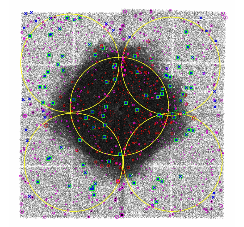
Figure 1: The Chandra image of CDF-S plus ECDF-S. X-ray detected sources are marked with red (CDF-S) and magenta (ECDF-S) circles, while optically selected Ly$\alpha$ emitters (LAEs) are marked with blue “X” s. Those LAEs selected for our stacking analysis are marked by green boxes. The large yellow circles presented the selection area (off-axis angle $\theta<$ 8′) in each ACIS-I image where we considered LAEs for inclusion in our analysis.

In this paper we focus on the X-ray data with an off-axis angle $<8\arcmin$, because the spatial resolution of ACIS-I data degrades rapidly for off-axis angles $>8^{\prime}$. This excludes 22 LAEs from our sample, leaving a total of 91 LAE at $z\sim 4.5$ covered by Chandra images with off-axis angle $\theta$ $<$ 8′. Of these, 22 are covered by the 2 Ms CDF-S exposure, and 86 by the shallower ECDF-S exposures, with 17 sources covered by both (see Figure 1). We choose a radius of 3″ to match X–ray counterparts to our LAE sample, as our narrowband data has a seeing of 0.9″  and the radius of 50% PSF regions of Chandra ACIS-I reaches 2.8″ at the edge of our selection area. Only one LAE (J033127.2-274247) has an individually detected X-ray counterpart (ECDFS-J033127.2-274247), with a spatial offset $\leq$ 0.4″ between the NB673 and X-ray coordinates. This object has previously been spectroscopically identified as an unobscured z $=$ 4.48 quasar (Treister et al. 2009), with full–band luminosity of L_0.5-10keV= 4.2 $\times$ 10⁴⁴ ergs s^-1 (assuming $\Gamma$ = 1.4, Lehmer et al. 2005). We measured the $f_{Ly\alpha}/f_{0.5-10keV}\approx 0.065$, consistent with expectations from a quasar template ($f_{Ly\alpha}/f_{0.5-10keV}$ $\sim$ 0.05, Sazonov et al. 2004).

There are two LAEs (J033204.9-280414 and J033154.1-274159) located in 95% PSF circles of two ECDF-S sources with offsets between X-ray and optical of 4.5″ and 4.1″, respectively. These offsets are too large to reliably associate the Ly$\alpha$ and X-ray sources, thus we do not classify them as X-ray detections, and we exclude these sources from our X-ray stack (Sec. 3.2).

We plot the X-ray signal-to-noise ratio distribution of the remaining X-ray flux measurements in Figure 2. This comprises 106 exposures on 88 distinct LAEs (22 are covered by the 2 Ms CDF-S exposure, and 84 by the shallower ECDF-S exposures, with 17 sources covered by both and one by two ECDF-S pointings, see Figure 1). The S/N ratios were calculated as $S/N=S/(\sqrt{T+0.75}+1)$ (Gehrels 1986), where $S$ and $T$ are the net counts and total counts extracted from their 50% PSF circles at 0.5-2, 2-7 and 0.5-7 keV bands, respectively. When converting from PSF-corrected count-rate to flux, the full and hard bands were extrapolated to the standard upper limit of 10 keV. All X-ray fluxes have been corrected for Galactic absorption (Dickey & Lockman 1990). To convert from X-ray counts to fluxes, we have assumed powerlaw spectra with photon index of $\Gamma$ = 2 (except where explicitly stated otherwise), which generally represents the X-ray spectra of both starburst galaxies and type 1 AGNs. For the LAEs without individual X-ray detections, we derived $3-\sigma$ upper limits to their X-ray fluxes (see Figure 4).

3.2 Stacking analysis

To determine the mean X-ray properties of the high–redshift LAEs that are too weak to be directly detected, we employed a stacking technique similar to that described in Wang et al. (2004) and Laird et al. (2006). The only difference was on the count-extraction, we chose the 50% PSF regions here for the nondetections rather than 80% PSFs (as in Wang et al) or fixed radius of 1.5$\arcsec$ (as in Laird et al). Small apertures give better upper limits on non-detections, and constant size is difficult for flux estimation here. After masking out the detected X-ray sources, the net and background counts were measured in the CDF-S and ECDF-S separately (see Figure 1 and Table 1). We computed two stacks: (a) The CDF-S data alone, and (b) all available data (CDF-S and ECDF-S). For objects in the overlap between the CDF-S and ECDF-S coverage, only their CDF-S data was included in stack (a), while data from both images was included in stack (b).

A marginal signal was found from the stacking of the CDF-S data in the soft band, while no signals were found in the other band of CDF-S or from the ECDF-S stacking. When cumulating the 22 LAEs in the central CDF-S in the soft X-ray band, we measure net and background counts of 26.6 and 74.4, which yields a signal–to–noise (S/N) = 2.4, with an effective exposure time of $\sim$ 36 Ms. The net counts and exposure time can be converted to an average flux of $F_{0.5-2.0keV}$ = 8.8$\pm$3.7 $\times 10^{-18}$ ${\rm\,ergs\,cm^{-2}\,s^{-1}}$. Including the ECDF-S data, the net exposure rises to 52 Msec for 106 exposure of 88 objects, while the net and background counts only increased 0.2 and 26 at soft band, respectively, corresponding to a slightly decreased S/N of 2.2. In principle, the increase in effective exposure of a factor 1.44 (52Ms/36Ms) should imply an expected value of S/N = 2.4$\times\sqrt{1.44}$ = 2.9. However, given the small numbers of X-ray photons involved, the count rates in the CDF-S and ECDF-S are in fact consistent at $<2\sigma$. The effective 52 Msec exposure decreases our soft band signal to $\langle f_{0.5-2}\rangle=6.4\pm 2.9\times 10^{-18}$ ${\rm\,ergs\,cm^{-2}\,s^{-1}}$, corresponding to an average luminosity of $\langle L_{0.5-2keV}\rangle$ = 1.3 $\times 10^{42}$ ergs $s^{-1}$ for LAEs at z $\sim$ 4.5, We also stacked the images of our LAEs together. Since the stacked samples in ECDFS were within their background fluctuations, we only stacked the 22 LAEs located in CDF-S. The resulting stacked image shows a signal consistent with the analysis above, which becomes apparent to visual inspection when smoothed with a Gaussian matched to the ACIS PSF size (see Figure 3).

We performed Monte Carlo simulations to check the significance of the stacked signal. By randomly choosing 22 positions on the source-masked CDF-S image, then cumulating source and background counts, we obtained distributions of both the net counts and the soft band S/N distribution (Figure 2). The net counts in the simulations agreed very well with a Poisson distribution having a mean of 74 (the expected total background counts in 22 apertures). Both the Monte Carlo simulation and the Poisson distribution gave a probability of P(S/N$<$2.4) = 99.83% for obtaining a signal as strong as the observed one by chance. We also use a jackknife test on our stacking result (see insets in fig. 2). This test is to validate the sample by using subsets of the data from which one or two sources have been excluded. The jackknife test shows that there are two sources that contribute about half of the stacked signal. We regard these as suspected X-ray sources.

We have recently obtained optical spectroscopy of $\sim$ 75% of our LAE sample (Zheng et al. 2010, in preparation), using the IMACS spectrograph on the Magellan 6.5m telescope, including the two LAE candidates (NB673-27 and NB673-62) which have S/N${}_{soft}>$ 1 in CDF-S and contributed about half of the X-ray signal. One (NB673-27) is confirmed as a low-redshift emission-line galaxy based on strong continuum flux blueward of the emission line. The other object (NB673-62) was confirmed as a LBG at z = 4.4 with little–to–no Ly$\alpha$ flux present. As our aim is to analyze the X-ray properties of the Ly$\alpha$ emitters at z = 4.5, we excluded these 2 objects in the following stacking analysis.The remaining 20 LAEs in the central CDF-S had net and background counts of 14 and 61, which yields a S/N = 1.4, with an effective exposure time of 32.7 Ms. Our Monte Carlo simulations gives a probability of P(S/N$<$1.4) = 96.03% for obtaining a signal as the observed one by chance. The stacked X-ray image of the 20 LAEs are also plotted in Figure 3, which is less distinguishable as being above the noise. We thus give a 3-$\sigma$ upper limit on the average flux as $\langle f_{0.5-2}\rangle<$ 1.6 $\times 10^{-17}$ ${\rm\,ergs\,cm^{-2}\,s^{-1}}$ for the 20 LAEs in CDF-S. Including the ECDF-S data, the effective exposure increases to 48.9 Ms, implying a decreased 3-$\sigma$ (1-$\sigma$) upper limit of average flux as $\langle f_{0.5-2}\rangle\leq$ 1.2 $\times 10^{-17}$ ${\rm\,ergs\,cm^{-2}\,s^{-1}}$ (6.3 $\times 10^{-18}$ ${\rm\,ergs\,cm^{-2}\,s^{-1}}$), corresponding to a luminosity of $\langle L_{0.5-2keV}\rangle\leq$ 2.4 $\times 10^{42}$ ergs $s^{-1}$ (1.2 $\times 10^{42}$ ergs $s^{-1}$).

4 DISCUSSION

4.1 Quasar contribution to LAEs

One LAE (J033127.2-274247) was detected in X-ray in ECDF-S, which was spectroscopically identified as a z = 4.48 unobscured AGN with Ly$\alpha$ luminosity of $L_{Ly\alpha}=2.4\times 10^{43}{\rm\,erg\,s^{-1}}$. This yields a direct high-z Ly$\alpha$ quasar density of 2.7${}^{+6.2}_{-2.2}\times$10^-6 Mpc^-3 (1 $\sigma$ Poisson error, Gehrels 1986), which is consistent with luminosity function (XLF) of AGNs at high-redshift (the comoving space density for all spectral type AGNs with 43 $<$ log L_x $<$ 45 at redshift 4 $<$ z $<$ 5 is 2.3$\times$10^-6 Mpc^-3, Yencho et al. 2009). Since Chandra ACIS does not have uniform sensitivity across the field of view, it is hard to directly get the fraction of galaxies hosting an quasar with X-ray luminosity above some value of Lx (e.g., see Figure 4, there are 3 LAEs with X-ray upper limit fluxes higher than the detected one in ECDF-S). If we only consider the LAEs in CDF-S, then the type 1 quasar fraction should be $\leq$5% with L_0.5-2keV $>2\times 10^{43}{\rm\,erg\,s^{-1}}$.

Following Wang et al. (2004) and Malhotra et al. (2003), we compare the X-ray to Ly$\alpha$ flux ratios of LAEs with three known high redshift type 2 quasars (see Figure 4), CDF-S 202 ($z$ = 3.7; Norman et al. 2002), CXO 52 ($z$ = 3.288; Stern et al. 2002), and HDFX 28 ($z$=2.011; Dawson et al. 2003), and with a type 1 quasar template derived from Sazonov et al. (2004). The Ly$\alpha$ selected AGNs at z = 4.5 (a type 1 AGN, this work), at z = 3.1 (a type 1 AGN, Gronwall et al. 2007), and at z = 2.25 (nine AGNs, Nilsson et al. 2009) are also plotted in figure 4. Since there are many values from different redshifts, the figure 4 is plotted in luminosity, and the soft X-ray luminosities are converted by assuming a photon index of $\Gamma$ = 2. We only consider the soft band observations because they are more sensitive than the total band 0.5-10 keV. Also, high redshift AGNs have effective power law indexes are often different, as $\Gamma=1.8$ (type 1 AGNs) or $\Gamma<1$ (type 2 AGNs). This introduces at least 50% difference in X-ray photometric flux normalization in the 0.5-10 keV band, but less than 10% in the 0.5-2 keV band (see Figure 2 of Wang et al. 2007). So in Wang et al. 2004, who choose $\Gamma$ = 2 to get the 1-$\sigma$ upper limit of 0.5–10 keV band flux to Ly$\alpha$ ratio of the z = 4.5 LAEs at LALA field, their type 2 AGN fraction of $<$ 4.8% should be 2 times larger, as $<$9.6% compared with type 2 AGN like CXO 52.

After scaling the X-ray luminosities with Ly$\alpha$ line luminosities, most of the Ly$\alpha$ selected AGNs are located within the region where type 1 and type 2 quasars are located. All the 20 LAEs in CDF-S are fainter in X-rays than HDFX 28, our type 1 quasar and Sazonov’s template, greater than 50% and 70% of them are fainter than CDF-S 202 and CXO 52. This indicates that about half of our LAEs at z $\sim$ 4.5 can be type 2 quasars like CDF-S 202. By comparing with LAEs in ECDF-S region, we can find that only CDF-S allow us to resolve almost all of the type 1 AGN, as well as some kind of type 2 AGN in our LAE sample. However, that average X-ray (1-$\sigma$ upper limit ) to Ly$\alpha$ ratio is 16 and 20 times below those of type 2 quasars like CDF-S 202 and CXO 52, and 31, 40 and 78 times below our LAE-QSO, the type 1 quasar template and LAE-QSO at z = 3.1. This implies that $<$ 6.3% of our LAEs can be type 2 AGNs like CXO 52 and CDF-S 202, and $<$ 3.2% of our LAEs can be type 1 quasar like our LAE-QSO.

4.2 SFR from X-ray and Escaping fraction of Lyman-$\alpha$ photon

The average flux (3-$\sigma$ upper limit) of our stacking analysis in the soft band corresponds to an average X-ray luminosity of $\langle L_{0.5-2keV}\rangle$ = 2.4 $\times 10^{42}$ ergs $s^{-1}$. If we assume that this is due to high mass X-ray binaries, using the empirical relation between the 0.5-2 keV luminosity and SFR of the nearby star-forming galaxies (Ranalli et al. 2003), we derive the upper limit of star formation rate as SFR${}_{X}\leq$ 530 M${}_{\sun}yr^{-1}$. This SFR is much higher than previously measured for LAEs. For comparison, Gronwall et al.’s X-ray undetected LAEs at z=3.1 can be translated to a 3-$\sigma$ upper limit of star formation rate of $<$ 70 M${}_{\sun}yr^{-1}$, only $\sim$13% of our upper limit SFR_X at z=4.5. If we adopt the more recent X-ray to star formation rate calibrations from Rosa-Gonzalez et al. (2009) and Mas-Hesse et al. (2008), based on the XMM-Newton observation and synthetic model of starbursts, respectively, the SFR upper limit estimated above will decrease by a factor of 1/3 $\sim$ 2/3. Even then it is more than 30 times larger than the SFR from the Ly$\alpha$ emission for our z $\sim$ 4.5 LAEs,which has a median of SFR_Lyα = 5.2 M_☉ yr^-1, compared to $\leq$ 10 times at z = 3.1 (Gronwall et al. 2007) and z = 2.1 (Guaita et al. 2010). Our larger upper limits stem from a combination of factors— the larger luminosity distance at $z=4.5$; a somewhat smaller sample; and the presence of a nearly-significant signal in our stack, which may indicate the presence of weak AGN among our sample.

Hayes et al. (2010) reported that the average escape fraction of Ly$\alpha$ photons $f_{esc,Ly\alpha}$ from star-forming galaxies at redshift z = 2.2 is $f_{esc,Ly\alpha}$ = (5.3 $\pm$ 3.8)% by performing a blind narrowband survey in Ly$\alpha$ and H$\alpha$. Since the X-ray emission from star-forming activities is essentially unaffected by IGM and intrinsic dust in the galaxy at high redshift, we can choose SFR_X as the upper limit of the unobscured intrinsic SFR. (SFR_X could over-estimate the intrinsic star formation in the case where AGN provide part of the X-ray flux.) Then we have SFR${}_{X}\geq$ SFR_intr , and SFR_Lyα = SFR${}_{intr}\times$ f${}_{IGM}\times$ f_esc,Lyα. Songaila (2004) measured the transmission of the Ly$\alpha$ forest produced by IGM up to redshift 6.3. The transmitted fraction f_IGM is $\sim$0.3 at redshift z = 4.5, and $\sim$0.7 at z=3.1. So we can get the lower limit of escaping fraction of Ly$\alpha$ photons as f${}_{esc,Ly\alpha}\sim$ 3.2% for z = 4.5 LAEs, and $\sim$ 9% for z = 3.1 LAEs with the SFR_X relation from Ranalli et al. (2003). The lower limit of f_esc,Lyα could rise by an additional factor of 2–3 based on the recent SFR_X calibrations from Rosa-Gonzalez et al. (2009) and Mas-Hesse et al. (2008), which show that more X-ray photons are produced through star-forming activities.

4.3 Existence of weak AGN in High-z Star-Forming Galaxies?

Any weak AGNs at high–redshift should be captured in the narrow-band surveys, provided their Ly$\alpha$ emission is strong enough. However, the AGN fractions among LAE samples reported in the literature refer to quasar fractions (L${}_{x}>4\times$ $10^{43}{\rm\,erg\,s^{-1}}$) for all samples at redshifts z $>$ 3. This is mainly due to the inadequate depths of X-ray exposures, apart from the two Chandra deep fields. At z $\sim$ 2.1, Guaita et al. did not report the X-ray luminosities, which can be as low as 10${}^{42}{\rm\,erg\,s^{-1}}$ in CDF-S. In the local universe, a large fraction of weak AGNs were reported based on multiple methods including X-rays (Finkelstein et al. 2009a). Although the LAEs of Gronwall et al. are located in the CDF-S where the X-ray luminosity is complete above 8$\times 10^{42}{\rm\,erg\,s^{-1}}$ at z $\sim$ 3.1, they only found one X-ray detected LAE in ECDF-S, with L_X = 2.8 $\times 10^{44}{\rm\,erg\,s^{-1}}$. They used a stacking analysis to derive a 3 $\sigma$ upper limit of 3.8 $\times 10^{41}{\rm\,erg\,s^{-1}}$ on the mean 0.5 - 2 keV luminosity of their LAEs. Their stacking is based on the old 1-Ms CDF-S, but when we repeated this stack using the 2-Ms CDF-S data, we also found no signal (S/N$<$1). The new data decreased the 3-$\sigma$ upper limit luminosity to 3.1 $\times 10^{41}{\rm\,erg\,s^{-1}}$ at z $\sim$ 3.1. In contrast, our $z\approx 4.5$ stacking analysis gives a 3-$\sigma$ upper limit luminosity to luminosity of $\langle L_{0.5-2keV}\rangle$ = 2.4 $\times 10^{42}$ ergs $s^{-1}$, where weak AGNs with luminosity of $\sim 10^{42}$ ergs $s^{-1}$ might be hidden.

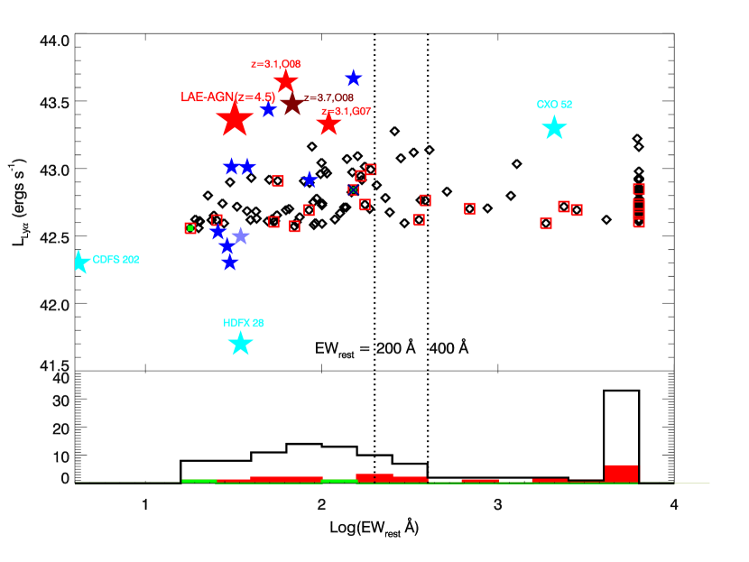
Figure 5: Top: Rest-frame EW vs. luminosity of Ly$\alpha$ line; Bottom: Rest-frame Ly$\alpha$ EW distribution. Black diamonds: all 113 LAEs at z = 4.5; Red squares: 22 LAEs in central CDFS; Green points: 2 LAE candidates in central CDFS which show S/N$>$1 and contribute about half of the stacking signal. The low-redshift interloper is marked with blue “X”; the other is likely a $z\approx 4.4$ Lyman break galaxy without strong Ly$\alpha$ emission. The filled red and blue stars are one Ly$\alpha$ selected AGN at z=4.5 (this work), one Ly$\alpha$ selected AGN at z=3.7 (Ouchi et al. 2008), two Ly$\alpha$ selected AGNs at z=3.1 (Gronwall et al. 2007 and Ouchi et al. 2008), and nine Ly$\alpha$ selected AGNs at z = 2.25 (Nilsson et al. 2009) , and X-ray selected three type 2 quasars are marked as cyan stars.

As mentioned in §1, AGNs could be the cause of high EWs of LAEs. The rest frame EW of two Ly$\alpha$ selected AGNs in CDF-S (see Figure 5) are $\sim$30Å (our work) and $\sim$100Å (Gronwall et al. 2007). In Subaru/XMM Deep field survey, Ouchi et al. (2008) reported two Ly$\alpha$ selected AGNs with rest frame EW of 60-70 Å at z = 3.1 and z =3.7. At z = 2.25, all the nine Ly$\alpha$ selected AGNs show a rest frame EW range of 25Å $<$ EW${}_{rest}<$ 160 Å (Nilsson et al. 2009). Although the intrinsic Ly$\alpha$ EW for AGN is uncertain, the rest-frame Ly$\alpha$ EWs of bright AGNs are typically in the range 50–150 Å (Charlot & Fall 1993, and references therein). Charlot & Fall (1993) show that AGNs which are completely surrounded by neutral hydrogen gas have rest-frame Ly$\alpha$ EWs of 827$\alpha^{-1}(3/4)^{\alpha}$ Å (ignoring absorption by dust), where $\alpha$ is the spectral index blueward of the Ly$\alpha$ line. According to the template of Sazonov et al. (2004), $\alpha$ = 1.7, which yields EW_rest $\sim$ 300 Å. Considering the scattering in the IGM, Dijkstra & Wyithe (2006) show the intrinsic distributuion of EW should be centred on EW_rest = 100 Å with $\sigma_{EW}$ = 30 Å. We also check the three type 2 quasars in Figure 5. Only type 2 quasars like CXO 52 would be selected as a LAE candidate with a large EW; the other two are either too faint or have an insufficient narrowband-to-broadband contrast to be selected as LAEs. Prior to examination of the optical spectra of our LAEs, only from the view of X-ray and optical images, we found that LAEs in CDF-S with EW_rest(Ly$\alpha$) $<$ 400Å dominate the signal as shown in Figure 3— indeed, this subsample has a soft band S/N as high as 2.7 (See Table 1). This is mainly due to the two LAEs which show S/N${}_{soft}>$ 1 (Figure 2) and contribute about half of the net counts. As mentioned in Sec. 3.2, spectroscopic results show that the two LAE candidates are not Ly$\alpha$ galaxies at $z\approx 4.5$. Excluding these two objects from the stack, the subsample with EW_rest(Ly$\alpha$) $<$ 400Å decreased to a S/N of 1.7. This level of signal could be simply a Poisson fluctuation in the photon statistics. Alternatively, it may be due to some low-luminosity AGN in the sample (as seen in the low-redshift Ly$\alpha$ selected AGNs at $z\sim 0.3$), or to star formation in the modest number of foreground and Lyman break galaxies that enter the sample. Low-luminosity AGN entering our sample could be either type 1 or type 2. The type 1 AGN are most likely confined to the EW_rest(Ly$\alpha$) $<$ 400Å  subsample, while the type 2 AGN show a larger dispersion in both EW_rest [Fig. 5] and other properties [Fig. 4]. This can be explained by the distinct mechanisms for the extinction of Ly$\alpha$ photons and the X-ray absorption for type 2 AGN, e.g., extinction of Ly$\alpha$ photons by Narrow Line Region and absorption of X-ray photons by dust torus. Then, most Ly$\alpha$ selected AGNs are likely to be hidden in the low EW_rest region.

5 Conclusion

Our work shows that X-ray observation is an effective method to identify AGN, as well as foreground objects in LAE samples. One X-ray detected LAE is spectroscopically confirmed as a type 1 quasar at z = 4.5. A stack of 22 other LAEs in the CDF-S field yields a marginal detection. However, two of these 22 sources contribute about half of the stacked X-ray signal, and these two were found to be a foreground interloper and a LBG at z=4.4 without strong Ly$\alpha$ emission. The mean flux of the remaining 20 sources, while positive, is not significantly different from zero. Including the ECDFS data, we obtain a $3\sigma$ upper limit on the average X-ray luminosity of 2.4 $\times 10^{42}$ erg s^-1. Compared to their average Ly$\alpha$ luminosity, we estimate that that fewer than 3.2% (6.3%) of our LAEs could be high redshift type 1 (type 2) AGNs, and those hidden AGNs might show low EW_rest. Using the relationship of X-ray emission and star-forming activity from low redshift star-forming galaxies, we obtained an upper limit on the unobscured SFR of SFR$<$ 180-530 M_☉ yr^-1. Compared to the SFR estimated from their average Ly$\alpha$ luminosity, we find a lower limit on the escape fraction of Ly$\alpha$ photons, f${}_{esc,Ly\alpha}>$ 3-10%. Doubling the depth of CDF-S X-ray observations is planned in 2010 and 2011 (see Chandra Electronic Bulletin 89). This will strengthen the power of X-ray diagnostics of LAEs, especially for revealing their unobscured SFR, for the new discovery of Ly$\alpha$ selected quasars and weak AGN, and for excluding the low-redshift contamination.

Table 1: Stacking results of undetected LAEs located in the ECDF-S and CDF-S Field with off-axis-angel $<$ 8′.

X-ray Field	Numbera	X-ray COUNTSb						FX($>3\sigma$)c			Time
		NetS	TotS	NetH	TotH	Net05-7	Tot05-7	Fsoft	Fhard	Ffull	Ms
ECDFS	83	0.2	26	-3.2	64	-3.1	90	1.44	7.49	3.98	16.2
ECDFS+QSO	84	11.9	38	-1.5	66	10.3	104	2.58	7.53	5.51	16.4
CDF-S	22	26.6	101	0.6	157	27.2	258	1.99	5.17	4.29	35.8
CDF-S∗	20	14	75	1.4	127	15.4	202	1.57	5.27	3.67	32.7
CDF-S (EW(Ly$\alpha$)${}_{rest}\geq$400Å)	10	1.8	36	3.0	73	4.8	109	1.6	9.8	5.1	15.8
CDF-S(EW(Ly$\alpha$)${}_{rest}<$400Å)d	12	24.8	65	-2.4	84	22.4	149	3.1	6.9	6.1	20.0
CDF-S(EW(Ly$\alpha$)${}_{rest}<$400Å)∗	10	12.2	39	-1.6	54	10.6	93	2.4	6.3	5.0	16.9
ECDFS+CDF-S∗	86	14.2	101	-1.8	191	12.3	292	1.17	3.92	2.71	48.9

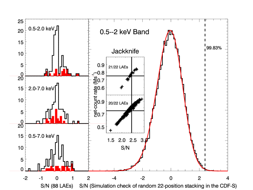
Figure 2: Histograms of the X-ray signal-to-noise ratios (S/N) for our selected 88 Ly$\alpha$ sources in three Chandra energy bands (Left; the 22 LAEs located in the CDF-S are filled with red colors), Jackknife tests on the 22 LAEs in the CDF-S at soft band (insets), and S/N distribution of Monte Carlo simulation by using 22 random locations (fake “sources”) in the CDF-S soft X-ray data(Right). The smooth red curve shows the distribution of S/N derived assuming a Poisson distribution of total counts in the aperture, with mean 74 (as in the real data). Both calculations yeild an $0.17\%$ chance of obtaining the observed signal by chance. See text for details.

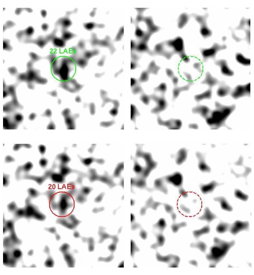
Figure 3: The stacked X-ray image of LAEs in central CDF-S. Top: 22 LAEs with the interloper; Bottom: 20 LAEs excluding the interloper and the LBG at z=4.4. Left: 0.5–2.0 keV band. Right: 2.0–7.0 keV band. The effective exposure time of the stacked images is $\sim$36 Ms for stacking 22 LAEs. The images are $\sim 20"\times 20"$ in size, and the circles are centered on the stacking position and have a radius of 2$"$. The images were smoothed using a Gaussian kernel having $\hbox{FWHM}=1.2^{\prime\prime}$, which approximates a matched filter for point sources detection given the $\sim 1^{\prime\prime}$ ACIS-I spatial resolution in these data. A marginal detection (S/N = 2.4) is seen at the top left panel, while excluding the two candidate LAEs which contribute about half of the marginal signal, the signal is no longer convincingly above the brightest noise peaks in the image (bottom left).

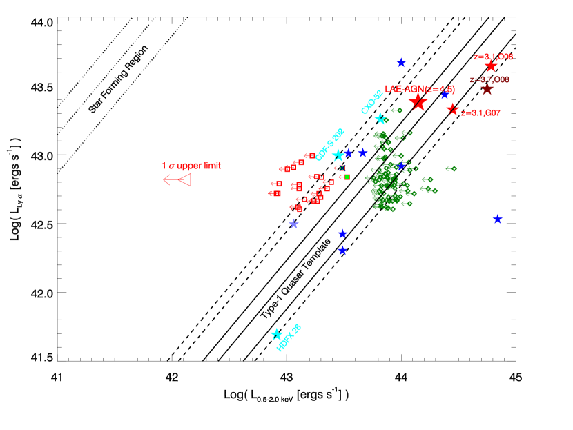
Figure 4: Ly$\alpha$ luminosities vs. 3 $\sigma$ upper limits of the soft X-ray luminosities for our LAEs (red squares: LAEs in CDF-S, dark-green diamonds: LAEs in ECDF-S) at z$\sim$4.5, compared with three known high-redshift type 2 quasars (cyan stars). All the soft X-ray luminosities are converted by assuming photon index $\Gamma$ = 2. Two LAE candidates in the central CDFS which show S/N$>$1 and contribute about half of the stacking signal are filled with green. These two are excluded during our analysis because one (marked with a blue “X”) appears to be a low-redshift interloper, while the other is likely a $z\approx 4.4$ Lyman break galaxy without strong Ly$\alpha$ emission. Diagonal lines indicate constant X-ray to Ly$\alpha$ flux ratios. The average X-ray to Ly$\alpha$ ratio for type 1 quasar template from Sazonov et al. (2004) is plotted as solid line, and the average X-ray to Ly$\alpha$ ratio for star-forming galaxies from Ranalli et al. (2003), Rosa-Gonzalez et al. (2009) and Mas-Hesse et al. (2008) are plotted as dotted lines. The red stars are the Ly$\alpha$ selected AGNs at z = 4.5 (this work), at z = 3.7 (Ouchi et al. 2008) and at z = 3.1(Gronwall et al 2007, Ouchi et al. 2008), and the blue stars are the Ly$\alpha$ selected AGNs at z = 2.25 (Nilsson et al. 2009, the one with light blue star is detected in hard X-ray band only, here the soft X-ray luminosity is the 1-$\sigma$ upper limit.) The empty red triangle is presented as the 1-$\sigma$ upper limit from stacking at the soft band.

References

- (1) Charlot, S. & Fall, M., 1993, ApJ, 415, 580
- (2) Colbert, E. M., et al. 2004, ApJ, 602, 231
- (3) Cowie, L. L., Barger, A.J., & Hu, E. M. 2010, ApJ, 711, 928
- (4) Dawson, S., McCrady, N., et al. 2003, AJ, 125, 1236
- (5) Dawson, S., Rhoads, J. E., Malhotra, S., et al. 2004, ApJ, 617, 707
- (6) Dawson, S., Rhoads, J. E., Malhotra, S., et al. 2007, ApJ, 671, 1227
- (7) Dickey, J. & Lockman, F., 1990, ARA&A, 28, 215
- (8) Dijkstra, M., & Wyithe, J.S.B., 2006, MNRAS, 372, 1575
- (9) Finkelstein, S. L., Cohen, S. H., Malhotra, S., Rhoads, J. E., et al. 2009a, ApJL, 703, 162
- (10) Finkelstein, S. L., Cohen, S. H., Malhotra, S., & Rhoads, J. E. 2009b, ApJ, 700, 276
- (11) Finkelstein, S. L., Rhoads, J. E., Malhotra, S., & Grogin, N. 2009c, ApJ, 691, 465
- (12) Finkelstein, S. L., Rhoads, J. E., Malhotra, S., Grogin, N., & Wang, J. X. 2008, ApJ, 678, 655
- (13) Gawiser, E., Francke, H., Lai, K., et al., 2007, ApJ, 671, 278
- (14) Gehrels, N. 1986, ApJ, 303, 336
- (15) Grimm, H.J., Gilfanov, M., & Sunyaev, R., 2003, MNRAS, 339, 793
- (16) Gronwall, C. et al. 2007, ApJ, 667, 79
- (17) Guaita, L., Gawiser, E., et al. 2010, ApJ, 714, 255
- (18) Hansen, M. & Oh, S. P. 2006, MNRAS, 367, 979
- (19) Hayes, M., Ostlin, G., et al. 2010, Nature, 464, 562
- (20) Hu, E. M., Cowie, L. L., et al. 2004, AJ, 127, 563
- (21) Iye, M., Ota, K, Kashikawa, N., et al. 2006, Nature, 443, 14
- (22) Lai, K., Huang, J. S., et al. 2007, ApJ, 655, 704
- (23) Laird, E.S., Nandra, K., et al. 2005, MNRAS, 359, 47
- (24) Laird, E.S., Nandra, K., Hobbs, A., & Steidel, C.C. 2006, MNRAS, 373, 217
- (25) Lehmer, B.D., Brandt, W. N., et al. 2005, ApJS, 161, 21
- (26) Lehmer, B.D., Alexander, D.M., et al. 2009, ApJ, 691, 687
- (27) Luo, B., Bauer, F. E., Brandt,W. N., et al. 2008, ApJS, 179, 19
- (28) Malhotra, S. & Rhoads, J.E. 2002, ApJL, 565, 71
- (29) Malhotra, S., Wang, J, Rhoads, J. E., et al. 2003, ApJ, 585, L25
- (30) Mas-Hesse, J. M., Oti-Floranes, H., & Cervino, M. 2008, A&A, 483, 71
- (31) Nilsson, K. K., Tapken, C., et al. 2009, A&A, 498, 13
- (32) Neufeld, D. A. 1991, ApJL, 370, 85
- (33) Norman, C. et al. 2002, ApJ, 571, 218
- (34) Ouchi, M., Shimasaku, K., et al. 2008, ApJS, 176, 301
- (35) Persic, M., Rephaeli, Y. et al. 2004, A&A, 419, 849
- (36) Pirzkal, N., Malhotra, S., Rhoads, J. E., Xu, C. 2007, ApJ, 667, 49
- (37) Ranalli, P., Comastri, A., & Setti, G. 2003, A&A, 399, 39
- (38) Rhoads, J. E., Malhotra, S., et al. 2000, ApJL, 545 85
- (39) Rhoads, J. E. et al., 2003, AJ, 25, 1006
- (40) Rosa-Gonzalez, D., et al. 2009, MNRAS, 399, 487
- (41) Sazonov, S.Y., Ostriker, J.P., & Sunyaev, R.A., 2004, MNRAS, 347, 144
- (42) Scarlata, C. et al. 2009, ApJL, 704, 98
- (43) Songaila, A. 2004, AJ, 127, 2598
- (44) Stern, D. et al. 2002, ApJ, 568, 71
- (45) Treister, E., Virani, S., Gawiser, E., et al. 2009, ApJ, 693, 1713
- (46) Venemans, B. P., et al. 2005, A&A, 431, 793
- (47) Wang, J. X., Rhoads, J. E., Malhotra, S., et al. 2004, ApJL, 608, 21
- (48) Wang, J. X., Malhotra, S., & Rhoads, J. E., 2005, ApJL, 622, 77
- (49) Wang, J. X., Zheng, Z. Y., Malhotra, S., et al. 2007, ApJ, 669, 765
- (50) Wang, J. X., Malhotra, S., Rhoads, J. E., et al. 2009, ApJ, 706, 762
- (51) Yencho, B., Barger, A., et al. 2009, ApJ, 698, 380