Statistics of 21-cm Fluctuations in Cosmic Reionization Simulations: PDFs and Difference PDFs

Abstract

In the coming decade, low-frequency radio arrays will begin to probe the epoch of reionization via the redshifted 21-cm hydrogen line. Successful interpretation of these observations will require effective statistical techniques for analyzing the data. Due to the difficulty of these measurements, it is important to develop techniques beyond the standard power spectrum analysis in order to offer independent confirmation of the reionization history, probe different aspects of the topology of reionization, and have different systematic errors. In order to assess the promise of probability distribution functions (PDFs) as statistical analysis tools in 21-cm cosmology, we first measure the 21-cm brightness temperature (one-point) PDFs in six different reionization simulations. We then parametrize their most distinct features by fitting them to a simple model. Using the same simulations, we also present the first measurements of difference PDFs in simulations of reionization. We find that while these statistics probe the properties of the ionizing sources, they are relatively independent of small-scale, sub-grid astrophysics. We discuss the additional information that the difference PDF can provide on top of the power spectrum and the one-point PDF.

1 Introduction: Cosmic Reionization and 21-cm Cosmology

The first stars and quasars reionized the intergalactic medium (IGM) during the epoch of reionization (EOR) (Barkana & Loeb, 2001). From the Ly$\alpha$ absorption in the spectra of distant quasars, we know that the EOR ended at $z\sim 6$ (see, e.g., Djorgovski et al., 2006), and from the cosmic microwave background (CMB) polarization maps we can infer that it started no later than $z\sim 15$ (Dunkley et al., 2009). Understanding how the reionization process developed over time offers a way to answer some of the critical questions of modern cosmology concerning properties of the first sources of light in the universe. Among the most promising observational probes of the EOR is the 21-cm spectral line, from hyperfine splitting in the ground state of hydrogen, with an energy of $5.9\times 10^{-6}$eV that corresponds to the rest-frame frequency of 1420 MHz. The redshifted 21-cm emission from neutral regions of the IGM during reionization is estimated to be a $1\%$ correction to the energy density of the CMB. It is expected to display angular structure and frequency structure, due to the inhomogeneities in the gas density, ionized fraction, $x_{i}$, and spin temperature (Madau et al., 1997) of the emitting gas.

Statistical detection of the large-scale brightness fluctuations is within the scope of a number of experiments that are presently being built, such as the Murchison Widefield Array (MWA) and the Low Frequency Array (LOFAR)(for reviews see, e.g., Furlanetto et al., 2006; Barkana & Loeb, 2007). In this context, it is important to develop appropriate statistical tools to be employed in analyzing the incoming data. Such development is facilitated by the fact that the N-body and radiative-transfer simulations of reionization have begun to reach the large scales of order 100 comoving Mpc (McQuinn et al., 2007; Iliev et al., 2008; Santos et al., 2008) needed to capture the evolution of the IGM during the EOR. These simulated data cubes can be used to test various statistical tools proposed for extracting information about the properties of the IGM during reionization.

So far, studies of the statistics of the 21-cm fluctuations have mainly focused on the power spectrum of the brightness temperature, $T_{b}$ (Bowman, Morales, & Hewitt, 2006; McQuinn et al., 2006). While this statistic is fully representative at the onset of the EOR, where the Gaussian primordial density fluctuations drive the 21-cm fluctuations, it ceases to be so at later times. Namely, as the reionization process advances, the mapping between the hydrogen density and $T_{b}$ becomes highly non-linear (as evidenced for instance by the bounded domain, $x_{i}\in[0,1]$), which results in non-Gaussianity of the probability distribution function (PDF) of $T_{b}$. For this reason, various authors have started exploring alternative and complementary statistics (e.g., Furlanetto et al., 2004; Saiyad-Ali et al., 2006), in particular the PDFs and difference PDFs of the 21-cm brightness temperature (Barkana & Loeb, 2008; Ichikawa et al., 2009). We test these two statistics on six different simulated data cubes from McQuinn et al. (2007). These data cubes are results of different astrophysical inputs that produce various reionization histories, all of which are allowed by the current observational constraints. We measure the one-point PDFs and difference PDFs and analyze their properties.

The plan of the paper is as follows: in Section 2.1 we briefly describe the simulation runs used in this paper. In Section 2.2 we then present the measured one-point PDFs along with the best fits of the model proposed by Ichikawa et al. (2009), and discuss the main parameters driving the PDF shape. We next present in Section 2.3 the first measurements of difference PDFs for the same set of simulations and analyze their properties. We conclude in Section 3.

2 Statistics of 21-cm Fluctuations

2.1 Simulations

In order to interpret future observations of the high-redshift universe, we need to understand the morphology of HII regions during reionization, in particular their size distribution and how it is affected by the properties of the ionizing sources, gas clumping and source suppression from photoheating feedback. For this purpose, McQuinn et al. (2007) ran a $1024^{3}$ N-body simulation in a box of size $65.6h^{-1}\simeq 94$ Mpc to model the density field, post-processing it using a suite of radiative transfer simulations. The authors assumed a standard $\Lambda$CDM cosmology, with $n_{s}=1$, $\sigma_{8}=0.9$, $\Omega_{m}=0.3$, $\Omega_{\Lambda}=0.7$, $\Omega_{b}=0.04$ and $h=0.7$. The outputs are stored at $50$ million year intervals, roughly between redshifts 6 and 16.

The radiative transfer code assumes sharp HII fronts, which are traced at subgrid scales. The properties of the sources are chosen in most cases so that reionization ends near z $\sim$ $7$. A soft ultraviolet spectrum that scales as $\nu^{4}$ is assumed for each source. The typical luminosity of a halo of mass $m$ is taken to be $\dot{N}(m)=3\times{10^{49}}m/({10^{8}}{M_{\odot}})$ ionizing photons per second. This corresponds to a halo star formation rate of $\dot{S}(m)=f_{\rm esc}^{-1}\,m/({10^{10}}{M_{\odot}})$ in units of $M_{\odot}\,{\rm yr}^{-1}$, for an escape fraction of $f_{\rm esc}$ and a Salpeter IMF. The N-body simulation resolves haloes down to ${10^{9}}{M_{\odot}}$, but since the effect of smaller mass haloes cannot be neglected, the effect of haloes down to ${10^{8}}{M_{\odot}}$ is included in some of the runs with a merger tree (see Table 1).

Simulation	Merger tree haloes	${\dot{N}}$ [photons sec-1]	Comments
$S1$	Yes	$2\times 10^{49}M_{8}$	-
$S4$	No	$C_{S4}M_{8}$	Includes only haloes with $m>4\times 10^{10}M_{\odot}$
$C5$	No	$6\times 10^{49}M_{8}$	Structure on small scales; $C_{\text{cell}}=4+3\delta_{\text{C}}$
$F2$	Yes	$2\times 10^{49}M_{8}$	Includes feedback on $m<M_{J}/2$; $\tau_{SF}=20\,\text{Myr}$
$M2$	No	$9\times 10^{49}M_{8}$	Includes minihaloes with $m_{\text{mini}}>10^{5}M_{\odot}$
$Z1$	Yes	$1\times 10^{50}M_{8}$	Higher source efficiency (early reionization)

Table 1: Details on the radiative transfer simulations from McQuinn et al. (2007). Merger tree haloes: ’Yes’ means that the halo resolution is supplemented with a merger tree down to $10^{8}M_{\odot}$. $C_{S4}$ is calibrated such that there is the same output of ionizing photons in each time-step as in S1. $M_{8}$ denotes the halo mass in units of $10^{8}M_{\odot}$. $C_{\text{cell}}$ is the subgrid clumping factor, and $\delta_{\text{C}}$ is the baryonic overdensity smoothed on the cell scale. $\tau_{SF}$ is the time-scale over which the cool gas in the source is converted into stars, and $M_{J}$ is the linear-theory Jeans mass.

For the purpose of measuring PDFs and difference PDFs, we choose six runs, labeled as in McQuinn et al. (2007): S1, S4, C5, F2, M2 and Z1. These runs differ by the efficiency of the sources and by the halo-mass resolution. Some runs include feedback from photo-heating, which suppresses source formation within ionized regions. Others investigate the impact of clumping, i.e., IGM density inhomogeneities, and include a subgrid clumping factor $C_{\text{cell}}$ different from unity. Finally, some runs account for the presence of minihaloes, which are dense absorbers for ionizing photons and thus tend to extend the process of reionization. A summary of the parameters of each of the six runs is presented in Table 1. The list of the redshift slices for each data cube is shown in Table 2. For more details about the simulations, see McQuinn et al. (2007).

Simulation	Redshift slices
$S1$	$6.9,7.3,7.7,8.2,8.7,9.4,10.1,11.1,12.3,13.9,16.2$
$S4$	$7.3,7.7,8.2,8.7,9.4,10.1,11.1,12.3,13.9,16.2$
$C5$	$6.6,6.9,7.3,7.7,8.2,8.7,9.4,10.1,11.1,12.3,13.9,16.2$
$F2$	$6.3,6.6,6.9,7.3,7.7,8.2,8.7,9.4,10.1,11.1,12.3,13.9,16.2$
$M2$	$6.9,7.3,7.7,8.2,8.7,9.4,10.1,11.1,12.3,13.9,16.2$
$Z1$	$10.1,11.1,12.3,13.9,16.2$

Table 2: List of the simulation runs and corresponding redshift slices discussed in this paper. The redshift outputs for each simulation are spaced in 50 Myr intervals.

2.2 One-point PDFs

We measure the one-point PDFs of the observed brightness temperature $T_{b}$ of the redshifted 21-cm emission, in the six simulation runs from McQuinn et al. (2007). We measure $T_{b}$ in a $32^{3}$ grid, i.e., $T_{b}$ is averaged over cells of size of 2.9 comoving Mpc, at each of the redshifts listed in Table 2. Note that this scale is much larger than the simulation’s spatial resolution; it is chosen by balancing the requirement to be large enough to fall close to the general range of the upcoming observations (corresponding to a resolution of arcminutes), with the need to be small enough compared to the simulation box to give a reasonable statistical sample. The PDFs are shown in Figure 1.

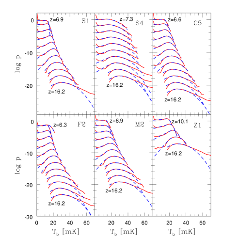
Figure 1: One-point PDFs for six different simulation runs, at the redshifts listed in Table 2. The $y$-axis is the logarithm of $p(T_{b})$, where $p$ represents the number fraction of points (i.e., pixels, or data-cube cells) at a given $T_{b}$, normalized by the temperature-bin size. The units of $p$ are mK^-1. There are $20$ evenly spaced temperature bins in each curve. The size of a bin at each redshift is set by the temperature range of the cells at that redshift. The top PDF in each plot is at the lowest redshift of the data cube, and the redshift increases downward. The $i$-th PDF in each plot is shifted down the vertical axis by $2(i-1)$ in logarithmic space, for clarity. We show the measured PDFs (solid red curves) as well as the best fits of the GED model (dashed blue curves).

As seen in Figure 1, the one-point PDFs are Gaussian-like at the highest redshifts and highly non-Gaussian at lower redshifts. The Gaussian shape of the PDFs at the beginning of reionization, when the universe is almost completely neutral, is driven by the primordial fluctuations in the density field of the emitting IGM gas. At lower redshifts and near the end of reionization, the completely ionized gas does not emit at 21-cm, while the brightness temperatures of the leftover patches of neutral gas are still governed by the density field inhomogeneities. At these redshifts, entirely ionized cells contribute to the increasingly-dominant delta-function at $T_{b}=0$ mK, while the emission from the partially neutral cells maintains a Gaussian around a higher $T_{b}$. The interplay between these two types of cells sets the shape of the PDFs as the reionization proceeds.

In Figure 1, we also plot the best fit of a Gaussian + Exponential + (Dirac) Delta function model (GED model) for the 1-pt PDFs. This is an “empirical” model (i.e., based on simulation data), suggested by Ichikawa et al. (2009):

$${p(T_{b})}=\left\{\begin{array}[]{cl}P_{D}\delta_{D}(T_{b})+a\;{{\text{e}}^{\lambda T_{b}}}\ ;&T_{b}\leqslant{T_{L}}\ ,\hfill\\ {c_{G}}\;{{\text{e}}^{-\frac{{{{(T_{b}-{T_{G}})}^{2}}}}{{2\sigma_{G}^{2}}}}}\ ;&T_{b}>{T_{L}}\ .\hfill\end{array}\right.$$ (1)

To get a smooth curve, the values of the two functions and their first derivatives are matched at the brightness temperature $T_{b}=T_{L}$, leaving (after normalization) four independent parameters for the GED model: the joining point of the exponential and the Gaussian function, $T_{L}$, the mean of the Gaussian, $T_{G}$, its standard deviation, $\sigma_{G}$, and its maximum value $c_{G}$.

From the best fit of the GED model to the PDF in each redshift slice for each of the simulated data cubes, we obtain the value of the probability fraction contained in the delta-function (at $T_{b}$’s around zero), $P_{D}$, in the Gaussian (at high $T_{b}$’s), $P_{G}$, and in the exponential part of the model (which interpolates between the delta function and the Gaussian), $P_{E}$. These parameters can be reconstructed from observations and must sum to unity, to ensure a normalized PDF. The variation of $P_{D}$, $P_{E}$, $P_{G}$, $T_{G}$, $T_{L}$, and $\sigma_{G}$ with the global ionized fraction, $\bar{x}_{i}$, is shown in Figure 2. The evolution of $\bar{x}_{i}$ with redshift for each of the simulation runs is also shown.

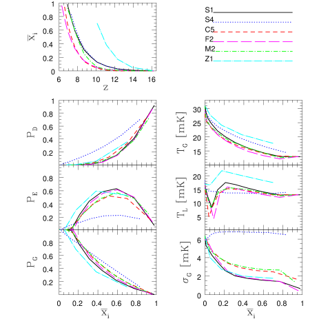
Figure 2: Top panel: evolution of the global ionized fraction $\bar{x}_{i}$ with redshift $z$, for each of the six simulation runs. Other panels show how various parameters derived from the best-fit GED model to the 21-cm PDF evolve as the reionization proceeds. $P_{D}$, $P_{E}$, and $P_{G}$ are, respectively, the fractional probability in the delta-function, the exponential, and the Gaussian part of the PDF; $T_{L}$ is the joining point of the exponential and the Gaussian, $T_{G}$ is the mean of the Gaussian, and $\sigma_{G}$ is its variance. There are four free parameters in the fit to each PDF.

When we fit the GED model, while its $\delta_{D}$ function portion is meant to capture the PDF spike near $T_{b}=0$ mK (at low redshifts), we do not attempt to model (or resolve in the data) the shape of this spike. Thus, we exclude the lowest temperature bin before fitting the GED model, and derive $P_{D}$ in three different ways: from the required overall normalization of the PDF to unity; then also directly, i.e., without the model fitting, from the total number count in the first bin of the $T_{b}$ PDF; finally, we measure the one-point PDFs of $x_{i}$, and estimate $P_{D}$ from the number count in the highest bin of this PDF (the cells in this bin have $x_{i}\geq 0.95$). These three different estimates of $P_{D}$ are compared for all six simulation runs in Figure 3. In this Figure, we show that the difference in $P_{D}$ calculated from the cell counts and from the GED model is negligible, which indicates that this model represents the data faithfully. The values of $P_{D}$ as measured indirectly (from fitting the GED model) yield an accurate estimate of the fraction of fully ionized cells. In the limit of infinite resolution, $P_{D}$ would equal $\bar{x}_{i}$ and so directly measure the reionization history, while in reality $P_{D}$ measures a low-resolution, smoothed-out version of the reionization history.

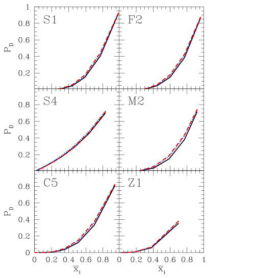
Figure 3: Three different measurements of $P_{D}$ are shown versus $\bar{x}_{i}$. These include $P_{D}$ as calculated from the best fit of the GED model (solid black curve), directly from the measured PDF of $T_{b}$, i.e., the fraction of pixels that fall within the lowest-temperature bin (dotted blue curve), and directly from the measured PDF of $x_{i}$, i.e., the fraction of pixels that fall within the highest-$x_{i}$ bin (dashed red curve). Results for the six different simulation runs are shown.

Comparing the various simulation runs, we find that small-scale structure has a relatively minor effect on the 21-cm PDF during reionization, at least for the present implementation of sub-grid astrophysics, and when the final reionization redshift is held (relatively) fixed. Compared to our fiducial case (S1), we have three simulations where mainly the small-scale structure has been adjusted: a scenario with photoheating feedback (F2), one with evaporating minihaloes (M2), and one with increased sub-grid clumping (C5). The latter two also do not have merger-tree source haloes. Figures 1 and 2 show that these scenarios have the effect of stretching out cosmic reionization, especially by delaying its progress early on, when the rarity of high-mass haloes makes feedback effective (F2), or the still-high density makes recombinations important (C5), or the minihaloes have not yet photo-evaporated (M2). However, in all these scenarios, the 21-cm PDF at a given stage (as measured by $\bar{x}_{i}$) is fairly unchanged. In particular, the evolution of the probabilities $P_{D}$, $P_{E}$, $P_{G}$, and the parameters $T_{G}$ and $T_{L}$ is rather similar for these three scenarios and S1.

Strong changes in the properties of the ionizing sources do have more of an effect on the evolution of the PDF. For example, a higher source luminosity (Z1) leads to earlier reionization by somewhat more massive haloes. Even early in reionization, the ionized bubbles are already rather large (compared to the fixed pixel scale at which the PDF is measured), which changes the PDF shape and the reconstructed GED-model parameters. Also, since reionization in this case occurs at higher redshifts, when the universe is denser, the mean 21-cm brightness is higher, leading to higher values of $T_{G}$ and $T_{L}$ compared to the lower-redshift cases. Furthermore, even without changing the redshift range, if the ionized sources lie in much more massive haloes (S4) than in the S1 case, the impact on the PDFs is noticeable. In this case, the ionized bubbles (produced by larger and more strongly-clustered sources) grow larger than the effective PDF resolution quite early in reionization, so that $P_{D}$ is larger than in the other cases (mostly at the expense of $P_{E}$), and is generally closer to the value of $\bar{x}_{i}$.

In summary, we find that $\bar{x}_{i}$ is the main parameter determining the one-point 21-cm PDFs. In particular, various modifications in the small-scale structure have only a minor effect on the PDF evolution versus $\bar{x}_{i}$ (as quantified by the parameters of the GED model fits). This suggests that analysis of features of the observed one-point PDFs can be used to reconstruct the global reionization history relatively independently of any assumptions about the astrophysics on unresolved sub-grid scales. On the other hand, the typical mass of source haloes, and the typical reionization redshift, have more of an effect. It is important to note, though, that observations will provide independent constraints on these major parameters. The redshift will obviously be measured, and, for example, the span of the reionization epoch will constrain the typical halo mass driving this process. Note also from Figure 2 that in all the simulation runs, the Gaussian probability $P_{G}$ can be taken as a rough estimate of the cosmic neutral fraction, $1-\bar{x}_{i}$.

While the one-point PDF is interesting, it will be rather difficult to measure with the upcoming generation of instruments, mainly due to comparatively bright foregrounds and the associated thermal noise. In particular, Ichikawa et al. (2009) found that the one-point PDF can only be reconstructed from upcoming observations if the analysis is made on the basis of quite strict (and not easily tested) assumptions that the real PDF is very similar in shape to that measured in numerical simulations. This difficulty motivates the use of an alternative statistical tool that should have a much higher signal-to-noise ratio for a given observation, namely the difference PDF proposed by Barkana & Loeb (2008). In the next Section we present the first numerical measurements of difference PDFs, specifically using the same six simulated data cubes, and we discuss their properties.

2.3 Difference PDFs

The PDF of the difference in the 21-cm brightness temperatures, $\Delta T_{b}\equiv|T_{b1}-T_{b2}|$, at two separate points in the sky (or, analogously, at two cells in the simulated data cube) was suggested by Barkana & Loeb (2008) as a useful statistic for describing the tomography of the IGM during the EOR. More precisely, if we consider two points separated by a distance $r$, then the distribution of $\Delta T_{b}$ is given by the difference PDF $p_{\Delta}(\Delta T_{b})$, normalized as $\int p_{\Delta}\Delta T_{b}=1$. The motivation for introducing this statistic is at least threefold. Firstly, the effective number of data points available for reconstructing the difference PDF is much larger than for the one-point PDF (by roughly a factor of the number of pixels over two, though the pixel pairs must be divided up into bins of distance $r$). Secondly, the difference PDF (which is a major piece of the two-point PDF) is a generalization which not only includes the information in the commonly considered power spectrum or two-point correlation function (which can be derived from the variance of the difference PDF), but also yields additional information. And thirdly, being a PDF of a difference in $T_{b}$, it avoids the mean sky background and fits naturally with the temperature differences measured via interferometry.

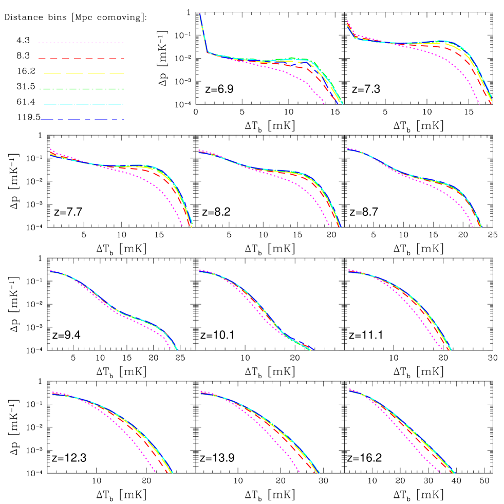
Figure 4: Difference PDFs are shown for all the output redshifts of the $S1$ simulation. The $x$-axis is the brightness temperature difference $\Delta T_{b}$ for pairs of cells, and the $y$-axis, $p_{\Delta}$, is the number fraction of pairs of cells at a given separation, $r$, with a given $\Delta T_{b}$ (normalized by the size of the $\Delta T_{b}$ bin). Different curves indicate different $r$ bins (the legend indicates the central values of the logarithmic bins).

We present the first measurements of difference PDFs, for the same set of McQuinn et al. (2007) simulation runs that we used to discuss the properties of the one-point PDF in the previous Section. The difference PDFs for all the redshifts of $S1$ are shown in Figure 4. For each of the other five simulation runs, we show difference PDFs at three representative redshifts in Figure 5. In Figures 4 and 5, every redshift has $6$ distance bins, logarithmically spaced, and each distance bin has $20$ temperature bins, linearly spaced. The range in distance is chosen so that it covers basically the full range from the resolution (pixel) scale to the largest separations found within the 94 comoving Mpc data cube.

Even for the one-point PDF, there is no good analytical model that matches simulations, probably because the PDF is sensitive to the reionization topology, specifically to the way in which the complex-shaped ionized bubbles partially overlap the box-shaped pixels. This led Ichikawa et al. (2009) to base their analysis on the PDF as measured in a simulation, and to consider an empirical model for fitting the PDF shape. Similarly, in the case of the difference PDF, the analytical model of Barkana & Loeb (2008) does not quantitatively match the result that we find in the simulations, but we can nonetheless use the model and the discussion in Barkana & Loeb (2008) to develop a qualitative understanding of the difference PDF and how best to analyze it.

At high redshifts, when the PDF is nearly Gaussian, the difference PDF (which is defined using the absolute value of $\Delta T_{b}$) should approximately be a half-Gaussian. Non-linear density fluctuations, though, give a slower decaying tail at high $\Delta T_{b}$ than would be expected for a pure Gaussian. As reionization develops with time, the difference PDF becomes a superposition of three contributing terms: The pixel pairs in which both pixels are fully ionized, those in which one pixel is (partly) neutral and the other ionized, and those where both are neutral. We explicitly show these three contributions in Figure 6 for one redshift near the midpoint of reionization in the $S1$ simulation. The both-ionized pixel pairs basically give the $\delta_{D}$ function at zero $\Delta T_{b}$; the amount of probability in this $\delta_{D}$ function is physically meaningful, as discussed below. The pairs in which one pixel is neutral and the other ionized tend to be well separated in $T_{b}$, and so this contribution is responsible for the high $\Delta T_{b}$ peak, at $\Delta T_{b}\sim 13$ mK in the case plotted here. As we consider smaller $r$, the $T_{b}$ values of the two points that are separated by $r$ become more strongly correlated, making it difficult for one to be ionized and the other neutral, and so this contribution declines at smaller $r$. At the same time, as we reduce $r$, this contribution becomes more highly concentrated at small values of $\Delta T_{b}$, since at small separations, if one pixel is fully ionized, then the second one tends to be at least highly ionized, making their $T_{b}$ difference small. Note also that the ionized+neutral contribution drops suddenly at $\Delta T_{b}\sim 1.5$ mK, but this is due to the fact that some of the probability in this region that should be included under ionized+neutral is incorrectly swept up under the both-ionized $\delta_{D}$ function, which is dominant at $\Delta T_{b}$ near zero. This is an unavoidable effect of the finite (2.9 Mpc) resolution of our gridded field. Since in practice we define a “fully ionized” pixel as having an ionization fraction of $95\%$ or higher, some highly ionized pixels are classified as fully ionized; a higher resolution map, with a definition closer to $100\%$ ionization, would move this artificial drop-off closer to $\Delta T_{b}=0$. Those pairs in which both pixels are neutral peak at $\Delta T_{b}=0$, and give a contribution with a roughly half-Gaussian shape, at all separations $r$.

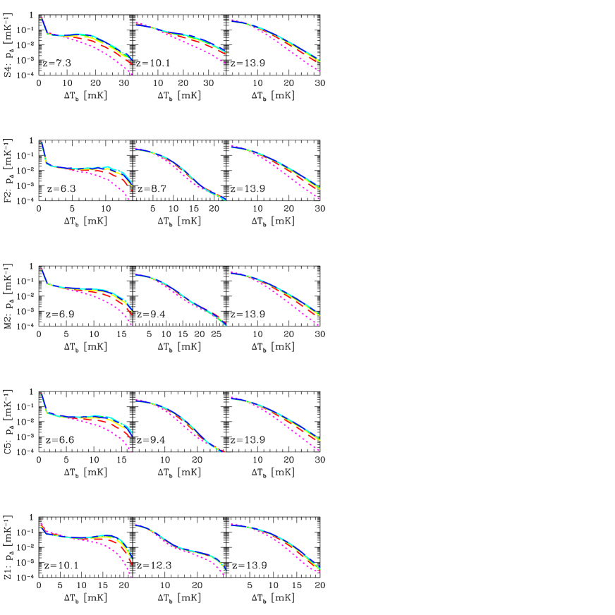
Figure 5: This Figure is a smaller version of Figure 4: difference PDFs for the rest of the simulation runs are shown for three representative redshifts (i.e., early, mid, and late reionization). The legend is the same as in Figure 4.

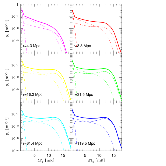
Figure 6: Separate contributions to the difference PDF, for the S1 simulation at $z=7.3$. We show the contribution of pixel pairs in which both cells are fully ionized (dashed curves, capturing the $\delta_{D}$ functions at zero $\Delta T_{b}$), pairs in which one cell is fully ionized (dot-dashed curves), and pairs in which neither of the cells is fully ionized (dotted curves). The total $p_{\Delta}$ (solid curves) is the sum of these three contributions.

The difference PDF as a function of separation transitions between two limits. The $r\to\infty$ limit corresponds to two uncorrelated points, for which $p_{\Delta}$ is essentially a convolution of the one-point PDF $p$ with itself. As long as $r$ is large enough to maintain a weak correlation, $p_{\Delta}$ keeps its large-$r$ limit and only varies slowly as $r$ is decreased. Once $r$ becomes small enough for a significant correlation (which is positive in the physical regimes considered here), it becomes harder to produce a large difference $\Delta T_{b}$ between the two correlated points (as noted above, even when one is fully ionized and the other is not); $p_{\Delta}$ thus becomes more strongly concentrated near $\Delta T_{b}=0$, approaching a $\delta_{D}$ function at $\Delta T_{b}=0$ as $r\to 0$.

The correlation between cells, referred to above, probes different physical effects at different redshifts. Before reionization, this is the density correlation, which arises from large-scale modes in the initial fluctuations. During reionization, the correlation of $T_{b}$ is dominated by ionization, so that points close enough together to be in the same ionized bubble (or in strongly correlated nearby bubbles) will have strongly correlated 21-cm brightness temperatures. Thus, by inspecting the plots, one can make a rough estimate of the average size of an ionized bubble at low redshifts, or the typical density fluctuation correlation length at high redshifts. This effective correlation length is the first separation bin at which the difference PDF at high $\Delta T_{b}$ drops significantly below its value at larger separations. For example, in Figure 4, the average bubble size can be seen to increase beyond 10 comoving Mpc during the late stages of reionization.

As in the case of the one-point PDF, the difference PDF is relatively insensitive to variations in the small-scale sub-grid physics, as tested by the various simulation runs. Figure 7 displays a comparison of the difference PDFs for the six different reionization runs, for various comoving distance bins, at the redshift where $\bar{x}_{i}$ is closest to the value of $0.4$ (i.e., in the midst of the reionization process). We also show the corresponding one-point PDFs, for easy comparison. Similarly to $p$ (as discussed in the previous section), the large ionized bubbles and correlation length in the case of reionization by massive, rare sources stretch $p_{\Delta}$ out to higher values of $\Delta T_{b}$ (as seen in the Z1 run and, especially, S4). Our findings are consistent with those of McQuinn et al. (2007) and with the general theoretical expectation that clustered groups of galaxies determine the spatial distribution of ionized bubbles (Barkana & Loeb, 2004) which is then driven by large-scale modes and is mainly sensitive to the overall bias of the ionizing sources.

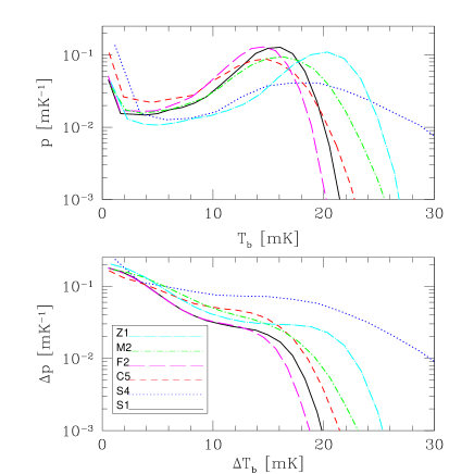
Figure 7: Comparison of the one-point PDFs (upper panel) and difference PDFs (lower panel), for all six simulation runs, at $r=16.2$ comoving Mpc. Each simulation run is shown at the redshift for which the value of the global ionized fraction $\bar{x}_{i}$ is closest to $0.4$, i.e. in the midst of the reionization process.

We next proceed to measure the parameter analogous to $P_{D}$, but this time for the case of difference PDFs. This parameter, which we denote $\Delta P_{D}$, represents the (number) fraction of pairs for which $\Delta T_{b}\approx 0$. In the reality of having limited resolution, it is the fraction of pairs for which $\Delta T_{b}$ falls within the lowest temperature bin. Ideally, this value would directly measure the fraction of pairs in which both cells are fully ionized, but the finite resolution adds a contribution from pairs that do not satisfy this condition, but nonetheless have matching brightness temperatures to within the bin size.

Just as $P_{D}$ in the one-point PDF measures a low-resolution version of the reionization history, so can $\Delta P_{D}$ be considered as measuring a low-resolution version of the ionization correlation function(Barkana & Loeb, 2008). In particular, in the limit of infinitely high resolution, $\Delta P_{D}$ would precisely measure the joint ionization probability of two points as a function of their separation. In this case, we would expect $\Delta P_{D}$ to vary from the corresponding value of $P_{D}$, at $r\to 0$, down to $P_{D}^{2}$, at $r\to\infty$ (where each pixel in the pair is independently ionized with probability $P_{D}$). While these relations are not exact with finite resolution, they do provide a rough guide for what to expect. We show the value of $\Delta P_{D}$ in Figure 8, for the redshifts of each simulation at which the $\delta_{D}$ function at $\Delta T_{b}\approx 0$ is visible. A comparison with the corresponding values of $P_{D}$ (shown in Figure 3) shows that the above theoretical behavior is satisfied only approximately, since the fully ionized pairs make up only a fraction of $\Delta P_{D}$. Still, the Figure shows the flat asymptote of $\Delta P_{D}$ at large $r$, and its rise as $r$ drops below the correlation length (although $r$ does not quite reach small enough values to see the flat $r\to 0$ asymptote).

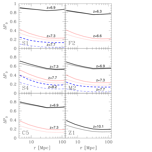
Figure 8: $\Delta P_{D}$ parameter, measured from difference PDFs as the value of the zero-temperature-difference bin, for the S1 simulation, is shown for the redshifts where it is non-vanishing. It represents the fractional probability in the delta function around $\Delta T_{b}\approx 0$, i.e. the number fraction of pairs of cells which are either both fully ionized, or both at the same brightness temperature. We see that this value tends to asymptote to the corresponding $P_{D}$, at $r\sim 0$, as expected for fully correlated cells. The thin lines of the same type and color represent the part of the corresponding $\Delta P_{D}$ that originates from pairs where both cells are fully ionized.

We have illustrated how the difference PDF encodes information about the EOR, in particular by separating out information on the ionization correlations (unlike the power spectrum analysis, in which the ionization and density correlations are mixed together). We leave for future work a more quantitative analysis of the features of the difference PDF and their relation to the properties of the ionizing sources and the reionization history.

3 Summary and Conclusions

Upcoming low-frequency radio observations will use the MWA, LOFAR, and similar instruments to survey the sky for redshifted 21-cm emission. It is therefore important to develop statistical tools that can be used to extract information about the history of reionization from these observations. In this paper, we examine PDFs and difference PDFs, using six different simulations from McQuinn et al. (2007). We show that the PDFs are highly non-Gaussian in the midst of the reionization process, and are thus a complementary statistic to the commonly discussed power spectrum. As a way to analyze the PDFs, we examine the evolution of the parameters of the best-fit GED model with the global ionized fraction $\bar{x}_{i}$. In particular, the $\delta_{D}$ function portion of the probability ($P_{D}$) measures a low-resolution, smoothed-out version of the reionization history (i.e., $\bar{x}_{i}$ as a function of redshift).

We also present the first numerical measurements of difference PDFs; specifically, we measure difference PDFs for the same set of simulation runs from McQuinn et al. (2007). We argue that the larger data set and the nature of this statistic can be significant advantages in the presence of bright foregrounds. The difference PDF can be physically understood as arising from three contributions: pixel pairs in which both, one, or neither of the pixels is ionized. As an illustration of the information that can be deduced from the difference PDFs, we consider the typical correlation length, which corresponds to the average size of an ionized bubble during reionization, or the typical density fluctuation correlation length, at the onset of the EOR. The difference PDF also has a delta-function portion ($\Delta P_{D}$), which measures a low-resolution, smoothed-out version of the ionization correlation function at each redshift.

We find that increasing small-scale clumping, and including photoheating feedback or minihaloes has only a small effect on the one-point and difference PDFs (considered at a given $\bar{x}_{i}$), at least within the range of assumptions covered by the simulations that we considered. On the other hand, the PDFs are highly sensitive to the properties of the ionizing sources, so that measuring them can help distinguish between reionization driven by large versus small haloes and help us unveil information about the first sources of light in the universe. These conclusions parallel those of McQuinn et al. (2007), highlighting the fundamental fact that the spatial structure of reionization is driven by large-scale modes and depends mainly on the overall bias of the ionizing sources (Barkana & Loeb, 2004; Furlanetto et al., 2004).

We plan to more precisely quantify the properties of difference PDF and establish the relation between their features and the properties of the IGM during the EOR. It would also be interesting to explore the PDFs and difference PDFs in alternative reionization scenarios, such as those dominated by X-ray sources or a decaying dark matter particle. Contrasting different scenarios may lead to a fuller understanding of the information content of the specific PDF shapes that we measured.

References

- Barkana & Loeb (2001) Barkana, R., & Loeb, A. 2001, Phys. Rep., 349, 125
- Barkana & Loeb (2004) Barkana R., Loeb A., 2004, ApJ, 609, 474
- Barkana & Loeb (2007) Barkana R., Loeb A., 2007, Rep. Prog. Phys., 70, 627
- Barkana & Loeb (2008) Barkana R., Loeb A., 2008, MNRAS, 384, 1069
- Bowman, Morales, & Hewitt (2006) Bowman J. D., Morales M. F., Hewitt J. N., 2006, ApJ, 638, 20
- Djorgovski et al. (2006) Djorgovski S. G., Bogosavljevic M., Mahabal A., 2006, New Astron. Rev., 50, 140
- Dunkley et al. (2009) Dunkley, J., et al. 2009, ApJ, 701, 1804
- Furlanetto et al. (2006) Furlanetto S. R., Oh S. P., Briggs, F., 2006, Phys. Rep., 433, 181
- Furlanetto et al. (2004) Furlanetto S. R., Zaldarriaga M., Hernquist L., 2004, ApJ, 613, 1
- Ichikawa et al. (2009) Ichikawa K., Barkana R., Iliev I., Mellema G., Shapiro P., 2009, arXiv:0907.2932
- Iliev et al. (2008) Iliev I. T., Mellema G., Pen U.-L., Bond J. R., Shapiro P. R. 2008, MNRAS, 384, 863
- Madau et al. (1997) Madau P., Meiksin A., Rees M. J., 1997, Astrophys. J., 475, 429
- McQuinn et al. (2006) McQuinn M., Zahn O., Zaldarriaga M., Hernquist L., Furlanetto S. R., 2006, ApJ, 653, 815
- McQuinn et al. (2007) McQuinn M., Lidz A., Zahn O., Dutta S., Hernquist L., Zaldarriaga M., 2007, Mon. Not. Roy. Astron. Soc., 377, 1043
- Saiyad-Ali et al. (2006) Saiyad-Ali, S., Bharadwaj, S., & Pandey, S. K., 2006, MNRAS, 366, 213
- Santos et al. (2008) Santos M. G., Amblard A., Pritchard J., Trac H., Cen R., Cooray A. 2008, ApJ, 689, 1