Mechanism for Spontaneous Growth of Nanopillar Arrays
in Ultrathin Films Subject to a Thermal Gradient

Abstract

Several groups have reported spontaneous formation of periodic pillar-like arrays in molten polymer nanofilms confined within closely spaced substrates maintained at different temperatures. These formations have been attributed to a radiation pressure instability caused by acoustic phonons. In this work, we demonstrate how variations in the thermocapillary stress along the nanofilm interface can produce significant periodic protrusions in any viscous film no matter how small the initial transverse thermal gradient. The linear stability analysis of the interface evolution equation explores an extreme limit of Bénard-Marangoni flow peculiar to films of nanoscale dimensions in which hydrostatic forces are altogether absent and deformation amplitudes are small in comparison to the pillar spacing. Finite element simulations of the full nonlinear equation are also used to examine the array pitch and growth rates beyond the linear regime. Inspection of the Lyapunov free energy as a function of time confirms that in contrast to typical cellular instabilities in macroscopically thick films, pillar-like elongations are energetically preferred in nanofilms. Provided there occurs no dewetting during film deformation, it is shown that fluid elongations continue to grow until contact with the cooler substrate is achieved. Identification of the mechanism responsible for this phenomenon may facilitate fabrication of extended arrays for nanoscale optical, photonic and biological applications.

I Introduction

The manufacture of ultra small optical and electronic components is nowadays based on optical lithography techniques whereby a geometric pattern defined by a photomask is transferred onto a photosensitive resist layer by exposure to UV light. Various chemical treatments are then used to embed the positive or negative image of this pattern onto a material film beneath the photoresist. While this commercial technique can generate feature sizes below 100 nm, there are certain disadvantages inherent in the patterning process Wallraff and Hinsberg (1999). For example, multiple step-and-repeat processes are required for deposition, exposure and removal of the photoresist layers for constructing three dimensional components. Inhomogeneities in the photoresist layer thickness, composition, exposure dose or developer concentration can cause significant surface roughness and scattering losses which diminish performance of optical or electronic components. Optical lithography is also inherently a two-dimensional technique whereby three dimensional components are fabricated layer upon layer. The process requires that the supporting substrates be rigid and flat, posing challenges for the fabrication of curved or complex shaped components. In an effort to eliminate such constraints while reducing fabrication time and cost, researchers have been exploring alternative, lower resolution patterning techniques such as ink-jetting Fuller et al. (2002), gravure printing Miller et al. (2003), direct-write Gratson et al. (2004), micro-moulding Heckele and Schomburg (2004) and nanoimprinting Chou et al. (1995); Guo (2007); Menard et al. (2007). These methods are more adaptable to new materials and pattern layouts; however, multiple etching steps are still required and device performance is still not comparable to those fabricated by conventional means. The materials of choice tend to be inks, colloidal suspensions and polymer melts del Campo and Arzt (2008), which are not only less costly but whose composition can be tuned to optimize functionality.

Some groups have been investigating less conventional means of film patterning by exploiting the self-assembling character of structures formed by hydrodynamic instabilities in thin films. Examples include dewetting induced by chemically templated substrates Zhang et al. (2003), capillary breakup on rippled substrates Petersen and Mayr (2008), island formation in ferroelectric oxide films Szafraniak et al. (2003), elastic contact instabilities in hydrogels Gonuguntla et al. (2006) and evaporative instabilities in metal precursor suspensions Cuk et al. (2000). The use of fluid instabilities for controlled formation of large area, periodic arrays provides an interesting approach for future development of non-contact, resistless lithography.

It is well known that liquid films with dimensions in the micron to nanometer range manifest exceedingly large surface to volume ratios. As such, small liquid structures can respond instantaneously to external modulation of surface forces. This sensitivity to surface manipulation has been successfully used to control the motion of small liquid volumes for micro-, bio- and optofluidic applications Darhuber and Troian (2005). For example, tangential stresses based on thermocapillary forces have been used to steer Darhuber et al. (2003a, b, c), mix Darhuber et al. (2004) and shape Dietzel and Poulikakos (2005) thin films and droplets on demand. Since the surface tension of liquids varies with temperature, thermal distributions can be applied directly to a supporting substrate to generate lateral gradients which drive the flow of liquid toward selected regions of a substrate. In this work, we examine systems comprising of liquid nanofilms subject to a transverse temperature gradient which have been observed to produce nanopillar arrays which grow and elongate in the direction of a cooler target substrate. The spontaneous formation of 3D large area arrays offers exciting possibilities for non-contact, resistless, one step fabrication of optical and photonic structures. Since solidification of the emergent molten structures occurs in-situ upon removal of the thermal gradient, it is anticipated that the resulting nanostructures will manifest specularly smooth interfaces, a distinct advantage for optical applications.

I.1 Formation of nanopillar arrays in molten polymer nanofilms

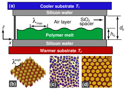
The typical experimental setup leading to spontaneous formation of nanopillar arrays is shown in Fig. 1(a). Polymers such as polystyrene (PS) or poly(metylmetacrylate) (PMMA) are first spun cast onto a clean, flat silicon wafer to an initial thickness $h_{o}$ of the order of a few hundred nanometers. The coated wafer is then overlay with a second silicon wafer containing vertical spacers along the periphery to ensure an air gap above the polymer film. The wafer separation distance, $d_{o}$, is normally several hundred nanometers. The bottom and top wafers are maintained at different temperatures above the polymer glass transition temperature to ensure a flowing liquid film. In all the experiments reported in the literature, $\Delta T=T_{2}-T_{1}\approx 10-50^{\textrm{o}}\textrm{C}$. Next, we review the experimental results of three independent groups reporting observations and measurements of nanopillars arrays.

Figure 1: (a) Sketch of experimental setup for formation of nanopillar arrays. Initial thickness of flat nanofilm is denoted by $h_{o}$; gap spacing in between silicon substrates is denoted by $d_{o}$. Length scale $\lambda_{\textrm{max}}$ represents theoretical prediction for pillar spacing; $\lambda^{\textrm{expt}}$ represents experimentally measured values. (b) AFM image of PMMA pillars Chou and Zhuang (1999): $h_{o}=95\>\textrm{nm}$, $d_{o}=260\>\textrm{nm}$, $\Delta T$ unknown, $\lambda^{\textrm{expt}}=3.4\>\mu\textrm{m}$. (c) Optical micrograph of PS pillars Schäffer et al. (2002): $h_{o}=100\>\textrm{nm}$, $d_{o}=285\>\textrm{nm}$, $\Delta T=46\>^{\textrm{o}}\textrm{C}$, $\lambda^{\textrm{expt}}=2.9\pm 0.6\>\mu$m. (d) AFM image of PMMA pillars Peng et al. (2004): $h_{o}=100\>\textrm{nm}$, $d_{o}=163\>\textrm{nm}$, $\Delta T=10\>^{\textrm{o}}\textrm{C}$, $\lambda^{\textrm{expt}}=6.5\>\mu\textrm{m}$.

I.1.1 Experiments by Chou et al. 

Chou et al. Chou and Zhuang (1999); Chou et al. (1999) appear to have been the first group to report nanopillar formation in ultrathin polymer films. In their experiments, they studied low molecular weight PMMA (approx 2K), which was first spun cast to a film thickness of 100 nm onto a cleaned silicon wafer and then annealed at $80\>^{\textrm{o}}\textrm{C}$ to drive off residual solvent. The annealed film was then placed within the assembly shown in Fig. 1(a), where the top wafer had been treated with a nonstick coating to prevent polymer attachment after solidification. The underside of the top wafer was either flat or patterned with a rectangular relief structure a few tens of microns in width and about $0.3\mu$m tall. In all experiments reported, there was no imposed temperature difference between the top and bottom wafers ($T_{2}-T_{1}=0$). Instead, the entire assembly was cyclically heated from room temperature to either $130\>^{\textrm{o}}\textrm{C}$ or $170\>^{\textrm{o}}\textrm{C}$, well above the polymer glass transition temperature $T_{\textrm{g}}=103\>^{\textrm{o}}\textrm{C}$ Mark (1996) to ensure a softened film. The heating cycle persisted for 5-80 minutes with no noticeable difference in pattern formation if the air gap was replaced by a vacuum at 0.3 Torr. In cases where the PMMA coated wafer was not overlay by a top wafer and simply exposed to open air, no protrusions were observed to form. When the top wafer was placed in close proximity to the melt surface i.e. $(d_{o}-h_{o})\approx 165\>\textrm{nm}$ , nanopillar arrays with in-plane hexagonal symmetry were obtained, as in the image shown in Fig. 1(b). These elongations were measured to have a diameter and pitch (i.e. pillary spacing) of a few microns; their overall height closely matched the gap distance $d_{o}$ separating the two wafers. AFM images of the resulting structures after solification revealed pillars with a flat top and fairly straight sidewalls. Chou et al. attributed the formation of these elongations to an image-charge induced electrohydrodynamic instability caused by non-uniform distribution of charges on the relief surface. Chou et al. also noted that thermal gradients might be playing a role but that Rayleigh-Bénard or Bénard-Marangoni cellular convection was unlikely since the initial film thicknesses were far too small to overcome the relevant critical numbers required for instability Chou et al. (1999).

I.1.2 Experiments and modeling efforts by Schäffer et al. 

Soon thereafter, Schäffer and co-workers Schäffer et al. (2002, 2003a); Schäffer (2001) used a similar setup as in Fig. 1(a) where the two confining wafers were purposely set to different temperatures such that $T_{2}>T_{1}$. They first spun cast high molecular weight films of PS ($T_{\textrm{g}}=95\>^{\textrm{o}}\textrm{C}$ Mark (1996), mol. wt. 108 kg/mol) dissolved in toluene onto a silicon wafer down to an initial thickness $80\>\textrm{nm}\lesssim h_{o}\lesssim 130\>\textrm{nm}$. It appears that these films were not annealed to drive out residual solvent after spin casting, which may have led to overestimates in the reported values of $h_{o}$ (discussed further in Section III). The wafer separation distance ranged from $100\>\textrm{nm}\lesssim d_{o}\lesssim 600\>\textrm{nm}$. The bottom wafer was then heated to $T_{2}=170\>^{\textrm{o}}\textrm{C}$; the top wafer was cooled to a temperature above $T_{\textrm{g}}$ such that $\Delta T=T_{2}-T_{1}$ ranged from $10\leq\Delta T\leq 55\>^{\textrm{o}}\textrm{C}$. The small wafer separation distances give rise to very large transverse thermal gradients of the order of $\Delta T/d_{o}\sim 10^{6}-10^{8}\>{}^{\textrm{o}}\textrm{C/cm}$. After subjecting the PS film to the thermal gradient overnight, the sample was quenched to room temperature and the top wafer removed. As in Chou et al. , the top wafer had been treated with a silanized monolayer in order to prevent adhesion of the PS. After solidification and removal of the top wafer, the films were observed to contain periodic nanopillar arrays, as shown in Fig. 1(c). To study the influence of the wafer separation distance $d_{o}$ on the pillar formation process, Schäffer et al. used a tilted plate geometry in all their experiments where the top wafer was inclined with respect to the bottom one by about $1\mu$m over a distance of 1 cm, corresponding to an inclination angle of about $0.0057^{\textrm{o}}$. This modification allowed simultaneous measurement of the array pitch as a function of $d_{o}$ within a single run. Schäffer et al. conducted a comprehensive set of experiments and determined the influence of the initial film thickness $h_{o}$, the wafer separation distance $d_{o}$, and temperature drop $\Delta T$ on the pillar separation distance $\lambda$. They ruled out any electrostatic effects by purposely grounding the confining wafers.

As noted both by Chou et al. Chou and Zhuang (1999) and Schäffer et al. Schäffer et al. (2003a), films ranging in thickness from millimeters to centimeters subject to a transverse thermal gradient are known to develop cellular instabilities which lead to periodic surface deflections at the air/liquid interface due either to Rayleigh-Bénard (RB) or Bénard-Marangoni (BM) convection Probstein (1994). These instabilities, however, generate very shallow corrugations and not pillar-like protrusions as observed in nanofilms. Onset of instability requires that the critical Rayleigh number $Ra_{\textrm{onset}}$ for buoyancy driven flow (which scales as $h^{4}_{o}$) or the critical Marangoni number $Ma_{\textrm{onset}}$ for thermocapillary flow (which scales as $h^{2}_{o}$) exceed 660 - 1700 or 50-80, respectively, depending on the boundary conditions. In the nanofilm experiments, the corresponding values are estimated to be $Ra\approx 10^{-16}$ and $Ma\approx 10^{-8}$, orders of magnitude less than required for onset of instability.

Schäffer et al. therefore proposed a different mechanism for instability and interfacial deformation based on a novel radiation pressure model. They hypothesized that low frequency acoustic phonons (AP) can reflect coherently from the interfaces of the molten film over distances of the order of the film thickness despite that the melt is in an amorphous state. These low frequency modes are postulated to generate a significant destabilizing radiation pressure while conducting little heat. By contrast, the high frequency modes are expected to propagate diffusively with little interfacial resistance and therefore little interfacial pressure. These modes, however, are essential for establishing the steady-state heat flux across the air and melt layers. The mechanism described represents a kind of acoustic analogue of the radiation pressure caused by optical phonon reflections in closely spaced metal plates placed in vacuum, known to generate the Casimir interaction force Morariu et al. (2004). Since the air/melt interface is liquid-like and therefore deformable, the acoustic phonons in the polymer melt are believed to generate an outwardly oriented radiation pressure, which counteracts the stabilizing force of surface tension; infinitesimal surface deflections can therefore grow into sizeable protrusions. Schäffer et al. developed a detailed hydrodynamic model based on the slender gap approximation for describing the evolution equation for the film thickness, $h(x,y,t)$. A linear stability analysis of this evolution equation leads to an analytic expression for the wavelength corresponding to the fastest growing unstable mode, namely

$$\lambda^{\textrm{AP}}_{\textrm{max}}=2\pi h_{o}\sqrt{\frac{\gamma\>u_{p}}{Q(1-\kappa)k_{\textrm{air}}\Delta T}}\left[\frac{d_{o}}{h_{o}}+\kappa-1\right]~{},$$ (1)

where $\gamma$ denotes the surface tension of the polymer melt, $u_{p}$ is the speed of sound in the polymer melt and $\kappa=k_{\textrm{air}}/k_{\textrm{melt}}$ denotes the ratio of thermal conductivity of air to that of the polymer melt. The superscript AP differentiates this expression from the one to be derived for a thermocapillary model (TC). The material constants in Eq. (1) are evaluated at the substrate temperature $T_{2}$. The parameter $Q$ represents the acoustic quality factor determined from the phonon reflection and transmission coefficients corresponding to the four media constituting the system, namely the bottom silicon wafer, the polymer melt, the overlying air layer and the top silicon wafer. Positive values of $Q$ lead to film destabilization and the formation of nanopillar arrays. Schäffer et al. compared the prediction for $\lambda^{\textrm{AP}}_{\textrm{max}}$ directly with the pillar spacings obtained in experiment, $\lambda^{\textrm{expt}}$. A least squared fit of the experimental data to the model with $Q$ and $u_{p}$ as fitting parameters produced good agreement (see dashed curves in Fig.3(b) ). In particular, it was shown that the value of $Q$ did not vary with $h_{o}$, $d_{o}$ or $\Delta T$. The acoustic quality factor $Q$ seemed to depend on the choice of substrate; $Q=6.2$ was obtained for the silicon/air/PS/silicon system, while $Q=83$ for films supported by a silicon wafer coated with a 100 nm layer of gold. Unfortunately, it was reported Schäffer (2001) that the measurements of $\lambda^{\textrm{expt}}$ included not only pillar formations but lamellar structures, spirals and other periodic formations caused either by defects in the initial film or by prolonged contact with the cooler substrate. In many cases, protrusions had undergone reorganization while in contact with the cooler wafer. In addition, measurements of pattern periodicity were obtained long after contact with the upper substrate and subsequent solidification. Comparison of these measurements to a model based on linear instability is therefore problematic.

Schäffer et al. concluded that they had uncovered a novel instability in nanofilms induced by a radiation pressure from interfacial reflections of low frequency acoustic phonons. They noted that the frequency dependence for propagation of acoustic phonons with large mean free path is highly unlikely in low molecular weight polymers and that the instability would not be observed in such systems since they lack the necessary glassy rheological response Schäffer et al. (2003a). In a separate study, Schäffer et al. Schäffer et al. (2003b) also conducted experiments with relief structures patterned with complex patterns held in close proximity to the polymer melt interface. The smallest values of $d_{o}/h_{o}$ lead to well defined replicas in the polymer film.

I.1.3 Experiments by Peng et al. 

Shortly following the work of Schäffer et al. , Peng and co-workers Peng et al. (2004) used a similar assembly as in Fig. 1(a) to study PMMA films with $h_{o}\approx 100$ nm, $T_{2}=160\>^{\textrm{o}}\textrm{C}$, $130\>^{\textrm{o}}\textrm{C}\leq T_{1}\leq 150\>^{\textrm{o}}\textrm{C}$ and $110\leq d_{o}\leq 210\>\textrm{nm}$. They were able to obtain nanopillar arrays after about $0.5-2.5\>\textrm{hrs}$; however, they did not conduct a parametric study nor compare their measurements of the pillar spacing with the prediction of Schäffer et al. . Fourier transforms of the nanopillar arrays showed well defined hexagonal symmetry in some cases, as shown in Fig. 1(d). In other experiments, the pillar formations adopted either stripe or spiral symmetry. Peng et al. used a simple energy minimization argument first introduced by Schäffer et al. to show that pattern selection between stripe and hexagonal arrangements is merely controlled by the thickness of the overlying air film, while spiral formations are likely caused by point defects in the film. In a final experiment, Peng and co-workers successfully transferred nanopillar patterns first formed in PMMA onto an elastomeric film of poly(dimethylsiloxane) (PDMS) i.e. negative replication of the original pattern. This demonstration outlined the ease with which potential patterns can be transferred into subsequent films for applications involving large area patterning.

I.2 Motivation for this study

In recent work Dietzel and Troian (2009), we re-examined the prevailing hypothesis for pillar formation in nanofilms based on coherent reflections of acoustic phonons in molten polymer nanofilms Schäffer et al. (2003a, b). Such a mechanism requires coherent phonon propagation of the order of the film thickness in an amorphous fluid layer. A review of the literature has shown that acoustic phonon mean free paths of the order of 10-100 nm have only been measured in solid polymer nanofilms at frequencies of order 100 GHz and at temperatures $-193^{\textrm{o}}\textrm{C}\leq T\leq 27^{\textrm{o}}\textrm{C}$ Morath and Maris (1996), far below the temperatures used in the experiments described above. Such long attenuation lengths, however, are highly unlikely in molten amorphous films far above $T_{\textrm{g}}$ because of the degree of disorder present and the enhanced mobility of polymer chains at temperatures above $T_{g}$.

Given that the free surface of thin liquid films is easily deformed by surface stresses Darhuber and Troian (2005), we instead demonstrate in this work that nanopillar formations are caused by the nanoscale analogue of the long-wavelength Bénard-Marangoni instability Scriven and Sternling (1964); Smith (1966); Oron et al. (1997); Vanhook et al. (1995), previously investigated for film thicknesses ranging from several hundred microns ($70\lesssim h_{o}\lesssim 270\>\mu\textrm{m}$ Vanhook et al. (1997, 1995)) to millimeters. In macroscopically thicker films, film protrusions caused by thermocapillary flow are stabilized by capillary and gravitational forces, such that only gentle surface deflections are possible Vanhook et al. (1997). Onset of instability in such films requires that the inverse dynamic Bond number $D^{\textrm{dyn}}_{\textrm{onset}}=\gamma_{T}\Delta T_{\textrm{film}}/\rho g{h_{o}}^{2}\geq 2/3(1+F)^{-1}$, where $\rho$ is the liquid density, $\gamma_{T}\equiv|d\gamma/dT|$, $\gamma$ is the liquid surface tension, $\Delta T_{\textrm{film}}$ is the temperature drop across the liquid layer, $F=(1-\kappa)/(D+\kappa-1)$ is an order one constant, $D=d_{o}/h_{o}$, and $\kappa=k_{\textrm{air}}/k_{\textrm{melt}}$. Estimates corresponding to the experiments of Schäffer et al. and Peng et al. indicate that $D^{\textrm{dyn}}\gtrsim\textsf{O}(10^{7})$ and $G\sim\textsf{O}(10^{-14})$. These critical values lie far beyond the regime previously investigated by Vanhook and co-workers Vanhook et al. (1997, 1995) in which $D^{\textrm{dyn}}_{\textrm{onset}}\sim\textsf{O}(10^{-1}-1)$ and $G\sim\textsf{O}(10^{-1}-10^{2})$. These estimates indicate that nanofilms dominated by thermocapillary flow should always undergo instability. In what follows, we therefore propose an alternative mechanism to the acoustic phonon model to help explain the formation of elongated structures in liquid nanofilms subject to a transverse thermal gradient. The analysis presented here indicates that the experiments conducted by Schäffer et al. and Peng et al. provide a rare window into the dynamics of the less common long-wavelength Bénard-Marangoni (BM) instability without interference from the better known short-wavelength (BM) instability, which gives rise to the beautiful cellular convection patterns often photographed.

There is an additional feature worth emphasizing in Fig. 1(a). In the absence of a top wafer, a transverse thermal gradient can still be established in a film heated from below by natural or forced convection within the gas layer above the polymer melt. Since the Biot number $\beta h_{o}/k_{\textrm{melt}}$ is linearly proportional to the polymer film thickness $h_{o}$ (where $\beta$ is the heat transfer coefficient for natural convection), however, this number will be small. As a result, the thermal gradient within the viscous film will also be small and thermocapillary stresses at the interface may be easily stabilized by capillary forces. This is probably the reason why no fluid elongations were observed in the experiments of Chou et al. in which the polymer melt was heated in open air. Use of a top substrate maintained at a cooler temperature held in close proximity to the melt surface enforces a sizeable transverse thermal gradient which can be used to maximize and control thermocapillary flow.

In this work we demonstrate that the predominance of thermocapillary forces along the free surface of molten nanofilms leads to a linearly unstable system which forms periodic protrusions no matter how small the applied thermal gradient in any liquid nanofilm, not just molten polymeric films. The analysis corresponds to a limiting case of Bénard-Marangoni flow peculiar to viscous films of nanoscale dimensions such that hydrostatic forces are completely negligible and deformation amplitudes are small in comparison to the array pitch. Predictions of the pillar spacing from the linear analysis as a function of the substrate separation distance reveals good agreement with experiment. Deviations are likely due to overestimates in the reported values of $h_{o}$ for unannealed films, uncertainties in the measured values of $d_{o}$ caused by the use of a tilted upper plate, and possible changes in wavelength caused by prolonged contact with the cooler substrate and film solidification prior to measurements of the array pitch. Finite element simulations of the full nonlinear equation are also used to examine the array pitch and growth rates beyond the linear regime. Inspection of the Lyapunov free energy as a function of time confirms that in contrast to typical cellular instabilities in macroscopically thick films, pillar-like elongations are energetically preferred in nanofilms. Provided there occurs no dewetting during film deformation, it is shown that fluid elongations continue to grow until contact with the cooler substrate is achieved. Identification of the mechanism responsible for this phenomenon may facilitate fabrication of extended arrays for nanoscale optical, photonic and biological applications.

II Evolution of molten nanofilms subject to the slender gap approximation

II.1 Films confined by parallel substrates

The molten layer is modeled as an incompressible Newtonian fluid since the flow speeds and shear rates inherent in the experiments described are very small. Consistent with the slender gap approximation, all lateral dimensions are scaled by the pillar spacing distance $L$, while all vertical scales are normalized by the initial film thickness $h_{o}$ such that $(X,Y)=(x/L,y/L)$, $Z=z/h_{o}$, $H(X,Y,\tau)=h(x,y,t)/h_{o}$ and $D_{o}=d_{o}/h_{o}$. The pillar spacing $L$ will later be identified with the wavelength of the maximally unstable mode, $\lambda_{\textrm{max}}$, obtained from linear stability analysis. The conservation equations for mass and momentum within the thin liquid film are given by

$$\partial U/\partial X+\partial V/\partial Y+\partial W/\partial Z=0$$ (2)

$$\epsilon Re\frac{DU}{D\tau}-\epsilon^{2}\left(\frac{\partial^{2}U}{{\partial X}^{2}}+\frac{\partial^{2}U}{{\partial Y}^{2}}\right)=-\frac{\partial P}{\partial X}+\frac{\partial^{2}U}{{\partial Z}^{2}}$$ (3)

$$\epsilon Re\frac{DV}{D\tau}-\epsilon^{2}\left(\frac{\partial^{2}V}{{\partial X}^{2}}+\frac{\partial^{2}V}{{\partial Y}^{2}}\right)=-\frac{\partial P}{\partial Y}+\frac{\partial^{2}V}{{\partial Z}^{2}}$$ (4)

$$\epsilon^{3}Re\frac{DW}{D\tau}-\epsilon^{2}\left(\epsilon^{2}\frac{\partial^{2}W}{{\partial X}^{2}}+\epsilon^{2}\frac{\partial^{2}W}{{\partial Y}^{2}}+\frac{\partial^{2}W}{{\partial Z}^{2}}\right)=-\frac{\partial P}{\partial Z}.$$ (5)

Equation (2) yields the scaling for the velocity components, namely $\overrightarrow{U}=(U,V,W)=(u/u_{\textrm{c}},v/u_{\textrm{c}},w/\epsilon u_{\textrm{c}})$, where $u_{\textrm{c}}$ represents the characteristic lateral speed set by thermocapillary flow. The corresponding Reynolds number based on the initial film thickness is $Re=\rho u_{\textrm{c}}h_{o}/\eta$, where $\rho$ and $\eta$ denote the polymer melt density and viscosity. In what follows, the polymer viscosity is assumed constant (i.e. a Newtonian fluid) and equal to $\eta=\eta(T_{2})$ foo . The non-dimensional Lagrangian or substantial derivative is denoted by $D/D\tau=\partial/\partial\tau+\overrightarrow{U}\cdot\nabla$ where $\tau=u_{\textrm{c}}t/L$. The overall (dimensionless) pressure in the fluid is given by

$$P=\epsilon h_{o}(p+\phi)/(\eta u_{\textrm{c}})$$ (6)

where $p$ is the (dimensional) capillary pressure and $\phi$ represents contributions from hydrostatic pressure (i.e. $\phi=g\>z$ where $g$ is the gravitational constant) and disjoining pressure (e.g. van der Waals forces).

Within the slender gap approximation, $\epsilon^{2}=(h_{o}/L)^{2}\ll 1$ and $\epsilon Re\rightarrow 0$; all terms on the left hand side of Eqs. (3) - (5) therefore vanish. In this limit, the pressure $P$ within the thin film is independent of the vertical coordinate $Z$. Equations  (3) and (4) can therefore be integrated with respect to $Z$, subject to the boundary conditions (BCs) at the liquid/solid and gas/liquid interface. Along the bottom substrate, it is assumed that the melt obeys the no-slip condition i.e. $\overrightarrow{U_{\parallel}}=(U,V)=0$. The dimensional stress jump across the air/melt interface Leal (2007), which accounts for both normal and tangential stresses, is given by

$$(\textbf{T}_{\textrm{air}}-\textbf{T}_{\textrm{melt}})\cdot\hat{n}+\nabla_{s}\gamma-\gamma\hat{n}(\nabla_{s}\cdot\hat{n})=0.$$ (7)

Here, $\textbf{T}=-(p+\phi)\textbf{I}+2\eta\textbf{E}$ denotes the total bulk stress tensor, where I is the unit tensor and E the rate of strain tensor, $\hat{n}$ denotes the unit vector outwardly pointing from the melt interface, $\nabla_{s}$ represents the surface gradient operator Deen (1998) and $\gamma$ is the surface tension of the polymer melt in air. Since the viscosity and density of air are negligible in comparison to those of the melt, $\textbf{T}_{\textrm{air}}=0$.

Thermocapillary flow within the melt leads to a non-vanishing shear stress $\nabla_{s}\gamma$ along the gas/liquid interface Leal (2007). After a straightforward derivation, it can be shown within the slender gap approximation Oron et al. (1997) that the tangential components of Eq. (7) reduce to

$${\partial U/\partial Z}|_{Z=H(X,Y,\tau)}=\partial\Gamma/\partial X$$ (8)

$${\partial V/\partial Z}|_{Z=H(X,Y,\tau)}=\partial\Gamma/\partial Y$$ (9)

where the surface gradient simplifies to $\nabla_{s}=\nabla_{\parallel}=(\partial/\partial X,\partial/\partial Y)$. The variable $\Gamma=\epsilon\gamma/(\eta u_{\textrm{c}})$ represents the dimensionless surface tension. The gradients in surface tension arise directly from thermal gradients along the melt interface i.e. $\nabla_{\parallel}\gamma=(d\gamma/dT)\nabla_{\parallel}T$. In dimensionless form, this relation is given by

$$\nabla_{\parallel}\Gamma=-\frac{\epsilon\gamma_{T}}{\eta u_{\textrm{c}}}\nabla_{\parallel}T|_{Z=H}=-\overline{Ma}\nabla_{\parallel}\Theta|_{Z=H}\,$$ (10)

where $\Theta=(T-T_{1})/(T_{2}-T_{1})$, $\gamma_{T}=|d\gamma/dT|$, $\Delta T=T_{2}-T_{1}>0$, and the Marangoni number $\overline{Ma}=\epsilon\gamma_{T}\Delta T/(\eta u_{\textrm{c}})$. In what follows, it is assumed that $T_{2}-T_{1}>0$; furthermore, for the liquid films of interest, the surface tension decreases linearly with increasing temperature $T$, which is reflected in the choice of the negative sign above.

The in-plane velocity components are therefore given by:

$$\overrightarrow{U}_{\parallel}=\left(\begin{array}[]{c}U\\ V\end{array}\right)=\left(\frac{Z^{2}}{2}-H\>Z\right)\nabla_{\parallel}P+Z~{}\nabla_{\parallel}\Gamma.$$ (11)

Equation (11) represents a linear superposition of pressure driven flow caused by variations in interfacial curvature and hydrostatic forces, as described by Eq. (15), and shear driven flow induced by thermocapillary stresses. Substitution of Eq. (11) into Eq. (2) followed by integration subject to the condition $W(X,Y,Z=0)=0$ gives the vertical component of the velocity field,

$$W=\left(\frac{HZ^{2}}{2}-\frac{Z^{3}}{6}\right){\nabla_{\parallel}}^{2}P+\frac{Z}{2}\left(\nabla_{\parallel}P\cdot\nabla_{\parallel}H-{\nabla_{\parallel}}^{2}\Gamma\right).$$ (12)

The evolution equation for the moving interface can then be determined by integration of Eq. (2) from $0\leq Z\leq H(X,Y,\tau)$ subject to $W(X,Y,Z=0)=0$ and the kinematic boundary condition, $W|_{Z=H}=DH/D\tau=\partial H/\partial\tau+\overrightarrow{U}|_{Z=H}\cdot\nabla_{s}H$. The Leibnitz rule for differentiation gives

$$\frac{\partial H}{\partial\tau}+\nabla_{\parallel}\cdot\left(\int^{H(X,Y,\tau)}_{0}\overrightarrow{U}_{\parallel}dZ\right)=0.$$ (13)

Substitution of Eq.(11) leads to the evolution equation for the melt interface $H(X,Y,\tau)$, namely

$$\frac{\partial H}{\partial\tau}+\nabla_{\parallel}\cdot\left(\frac{H^{2}}{2}\nabla_{\parallel}\Gamma-\frac{H^{3}}{3}\nabla_{\parallel}P\right)=0.$$ (14)

It is expected that the slender gap approximation remains valid throughout the growth process so long as $(d_{o}/L)^{2}\ll 1$, which holds for all the experiments described.

Since the pressure in the film is independent of $Z$ to order $\epsilon^{3}Re$, one can determine its value by considering the normal stress balance at $Z=H$. The normal component of Eq. (7) within the slender gap approximation yields the total pressure in the film to order $\epsilon^{2}$:

$$P=-\overline{Ca}\>^{-1}\nabla^{2}_{\parallel}H+\overline{Ca}\>^{-1}\>\overline{Bo}\>H,$$ (15)

where $\overline{Ca}=\eta u_{\textrm{c}}/(\gamma\epsilon^{3})$ and $\overline{Bo}=\rho gL^{2}/\gamma$. Parameter estimates from the experiments of Schäffer et al. indicate that $\overline{Ca}$ is of the order of $10^{1}-10^{2}$ [using Eq. (21)] while $\overline{Bo}$ is of the order of $10^{-5}-10^{-6}$. The hydrostatic contribution to the fluid pressure in Eq. (15) can therefore be neglected altogether. The influence of disjoining pressure arising from van der Waals interactions in films ranging from 10 - 100 nm in thickness Oron et al. (1997) is also ignored in this work. The flow induced by these molecular forces is weak in comparison to flow induced by thermocapillary stresses, which are of considerable magnitude in the experimental systems of interest. While disjoining pressure effects can be included in straightforward fashion within $P$, they are not the primary mechanism for instability. Furthermore, there is yet no consensus in the literature on the appropriate analytic form of the disjoining pressure in cases where films are subject to large thermal gradients; most of the simplified forms available in the literature are only appropriate for isothermal systems. It is also assumed that any thermocapillary effects caused by solvent evaporation and subsequent cooling of the interface Bestehorn et al. (2003) can be neglected. This assumption requires that solvent evaporation be completed (either naturally or by film annealing) before the film is inserted into the experimental assembly.

With these assumptions, the gradient of the Laplace pressure is given by

$$\nabla_{\parallel}P=-\overline{Ca}\>^{-1}\nabla^{3}_{\parallel}H-\epsilon^{2}\nabla^{2}_{\parallel}H\nabla_{\parallel}\Gamma.$$ (16)

The last term, which represents a correction to the Laplace pressure due to local variation in surface tension, scales as $\epsilon^{2}$ and can be safely ignored. The surface tension coefficient in the Laplace pressure only is therefore set to the value $\gamma=\gamma(T_{2})$.

Determination of the interfacial stress conditions in Eqs. (8) and (9) requires knowledge of the thermal distribution along $Z=H$, which can be obtained from the energy equations Oron et al. (1997) pertaining to the confined air/liquid bilayer shown in Fig. 1:

$$\epsilon RePr\frac{D\Theta}{D\tau}-\epsilon^{2}\left(\frac{\partial^{2}\Theta}{{\partial X}^{2}}+\frac{\partial^{2}\Theta}{{\partial Y}^{2}}\right)=\frac{\partial^{2}\Theta}{{\partial Z}^{2}}.$$ (17)

Here, the Prandtl number $Pr=\nu/\alpha$ refers to the kinematic viscosity $\nu$ and thermal diffusivity $\alpha$ of the corresponding air or liquid melt layer. The Reynolds number $Re$, defined previously, is based on the corresponding layer thicknesses. Despite that $Pr$ is of the order of $10^{8}-10^{9}$ for the polymer melts of interest, the small gap approximation coupled with the vanishingly small value of $Re$ (see Tables 1 and 2) ensures that the left hand side of Eq. (17) is completely negligible. In fact, the slender gap approximation is well satisfied in all the experiments described earlier since $\epsilon^{2}\ll 1$, $\epsilon\,Re\ll 1$ and $\epsilon RePr\ll 1$. The thermal analysis conveniently reduces to a one dimensional thermal conduction problem for heat flow across an air/liquid bilayer subject to isothermal boundary conditions at $Z=0$ and $Z=D_{o}$. The temperature distribution along the melt interface is therefore given by, $\Theta|_{Z=H}=(D_{o}-H)/[D_{o}+(\kappa-1)H]$. Substitution of this solution into Eq. (10) yields

$$\nabla_{\parallel}\Gamma=\frac{\kappa~{}\overline{Ma}~{}D_{o}\nabla_{\parallel}H}{[D_{o}+(\kappa-1)H]^{2}}.$$ (18)

Substitution of Eqn. (16) and (18) into Eq. (14) then yields the expression governing the motion of the air/liquid interface, namely

$$\frac{\partial H}{\partial\tau}\!+\!\nabla_{\parallel}\cdot\!\left[\frac{\kappa\,D_{o}\,\overline{Ma}\,H^{2}}{2\,[D_{o}+(\kappa-1)H]^{2}}\nabla_{\parallel}H+\frac{H^{3}}{3\,\overline{Ca}}\nabla^{3}_{\parallel}H\right]=0.$$ (19)

The characteristic scale for the lateral velocity, $u_{\textrm{c}}$, is set to the value established by thermocapillary flow, which can be obtained from Eq. (18) by letting the film thickness, slope and and interfacial stress be order one and equal to unity - i.e. $H=1$, $\nabla_{\parallel}H=1$, and $(\partial U/\partial Z)_{Z=H}=\partial\Gamma/\partial X=1$, such that

$$\overline{Ma}=\frac{(D_{o}+\kappa-1)^{2}}{\kappa D_{o}}.$$ (20)

Since $\overline{Ma}=\epsilon\gamma_{T}\Delta T/(\eta u_{\textrm{c}})$, the scale for $u_{\textrm{c}}$ becomes

$$u_{\textrm{c}}=\frac{\epsilon\,\kappa\,D_{o}\,\gamma_{T}\,\Delta T}{\eta\,(D_{o}+\kappa-1)^{2}}.$$ (21)

Table 1: Order of magnitude estimates for characteristic numbers used in the thermocapillary model extracted from the experiments of Schäffer et al. [22, 26]. Values of Pr for PS and PMMA at 170^oC were obtained from Refs. [25] and [42]. The constant value of capillary number, $\overline{Ca}$, results from the choice of thermocapillary velocity used to scale the flow speed, as discussed in the section following Eq. (30)

$\epsilon$		$10^{-3}\!-\!10^{-2}$
$Re$		$10^{-18}\!-\!10^{-17}$
$Pr$		$10^{8}\!-\!10^{9}$
$\overline{Ma}$		$10^{0}\!-\!10^{1}$
$\overline{Ca}$		$52.6$
$\overline{Bo}$		$10^{-5}\!-\!10^{-6}$

Table 2: Literature values for air and polystyrene melt [$M_{n}\approx 107\>\textrm{kg/mol}$ and $M_{w}/M_{n}=1.07$ where $n$ and $w$ denotes number avg and weight avg] used in the analysis and numerical simulations. All parameter values quoted are for $T=170\>^{\textrm{o}}\textrm{C}$, except for $\gamma$ and $\gamma_{T}$, which were only available for $T=180\>^{\textrm{o}}\textrm{C}$. For comparison, Schäffer et al. Schäffer et al. (2002, 2003a) used polystyrene melts for which $M_{n}\approx 108\>\textrm{kg/mol}$ and $M_{w}/M_{n}=1.03$.

				Air		PS
$\rho$		(kg/m3)		$0.829\>$[43]		$987\>$[25]
$\eta$		(Pa$\cdot$ s)		$2.48\cdot 10^{-5}\>$[43]		$2.5\cdot 10^{4}\>$[42]
$k$		[W/(m$\>{}^{\textrm{o}}\textrm{C}$)]		$0.036\>$[43]		$0.130\>$[25]
$\alpha$		(m2/s)		$4.25\cdot 10^{-5}\>$[43]		$6.45\cdot 10^{-8}\>$[25]
$\gamma$		($10^{-3}\>$N/m)				$31.53\>$[44]
$\gamma_{T}$		[$10^{-3}\>$N/(m$\>{}^{\textrm{o}}\textrm{C}$)]				$0.0885$ [44]

The evolution of film disturbances governed by thermocapillary effects, as given by Eq. (19), is compared to evolution by acoustic phonon radiation pressure, as proposed by Schäffer et al. . While their derivation is also based on the slender gap approximation, the acoustic phonon model neglects altogether any flow induced by tangential stresses due to interfacial thermal gradients. Instead, the Laplace pressure, is counteracted by a radiation pressure due to phonon reflections which causes protrusions to grow. The overall fluid pressure in the AP model is therefore given by

$$P=-\>\overline{Ca}\>^{-1}\nabla^{2}_{\parallel}H-\overline{Ca}\>^{-1}\overline{Q}/[D_{o}+(\kappa-1)H],$$ (22)

where $\overline{Q}=2Qk_{\textrm{air}}\Delta T/(u_{p}\gamma\epsilon^{2})$ and $Q$ is the acoustic quality factor described in the Introduction. Substitution of Eq. (22) into Eq. (14) (with $\nabla_{\parallel}\Gamma=0$ since thermocapillary effects play no role in the acoustic phonon model) yields the evolution equation proposed by Schäffer et al. :.

$$\frac{\partial H}{\partial\tau}+\nabla_{\parallel}\cdot\left[\frac{\overline{Q}~{}(1-\kappa)H^{3}}{3~{}\overline{Ca}~{}[D_{o}+(\kappa-1)H]^{2}}\nabla_{\parallel}H+\frac{H^{3}}{3~{}\overline{Ca}}\nabla^{3}_{\parallel}H\right]=0.$$ (23)

Values for the thermophysical properties of air and PS are listed in Table 2. Corresponding numbers for experiments with PMMA Peng et al. (2004) are of similar magnitudes.

II.1.1 Linear stability analysis of evolution equation

Equations (19) and (23) can be further analyzed by linear stability theory to provide an estimate of the fastest growing mode, the one most likely to be observed in experiment. Predictions of the corresponding wavelength are therefore expected to compare favorably with the pillar spacing measured in experiment if the proposed mechanism is correct.

The behavior of Eq. (19) is examined in the limit where an initially flat and uniform film of thickness $H=1$ (i.e. base state) is subject to an infinitesimal periodic perturbation of amplitude $\widetilde{\delta H_{o}}\ll 1$ and wave number $\overrightarrow{K}_{\parallel}$ where $|\overrightarrow{K}_{\parallel}|=K=2\pi L/\lambda$. Solutions of the form $H(X,Y,\tau)=1+\widetilde{\delta H_{o}}\>\exp[\beta(K)\tau]\exp[i\overrightarrow{K}_{\parallel}\cdot\overrightarrow{X}_{\parallel}]$ are substituted into Eq. (19), where $\overrightarrow{X}_{\parallel}=(X,Y)$, and all quadratic or higher order terms are neglected. The resulting expression for the growth rate is

$$\beta(K)=\left(\frac{\kappa D_{o}\overline{Ma}}{2(D_{o}+\kappa-1)^{2}}-\frac{K^{2}}{3\overline{Ca}}\right)K^{2}.$$ (24)

Disturbances for which $\beta(K)=0$ neither grow nor decay. This condition establishes the criterion for marginal (M) stability where the corresponding wave number, $K_{\textrm{M}}$, for the thermocapillary model, is given by

$$K^{\textrm{TC}}_{\textrm{M}}=\sqrt{\frac{3}{2}\frac{\kappa D_{o}\overline{Ma}\>\overline{Ca}}{(D_{o}+\kappa-1)^{2}}}.$$ (25)

Note that in the absence of any stabilizing hydrostatic terms as is the case with nanofilms, there always exists a band of wavenumbers $0<K<K^{\textrm{TC}}_{\textrm{M}}$ for which the film is linearly unstable, no matter how small the value of the imposed temperature gradient. This stands in sharp contrast to the thermocapillary instability in much thicker films Vanhook et al. (1995, 1997) for which $K_{\textrm{M}}=(3\>\kappa\>D_{o}\>\overline{Ma}\>\overline{Ca}/[2(D_{o}+\kappa-1)^{2}]-\overline{Bo})^{1/2}$. For thicker films, there exists a critical Marangoni number for onset of instability:

$$\overline{Ma}_{\textrm{onset}}=\frac{2}{3}\frac{\overline{Bo}}{\overline{Ca}}\frac{(D_{o}+\kappa-1)^{2}}{\kappa\>D_{o}}~{}.$$ (26)

This criterion is commonly expressed in terms of the inverse dynamic Bond number $D^{\textrm{dyn}}_{\textrm{onset}}=\gamma_{T}\Delta T_{\textrm{film}}/(\rho gh^{2}_{o})\geq 2/3(1+F)^{-1}$, where $\Delta T_{\textrm{film}}$ represents the temperature drop across the liquid layer [and not the temperature drop across the bilayer as defined in Eq. (26)] and $F=(1-\kappa)/(D_{o}+\kappa-1)$ is a constant of order one Vanhook et al. (1997). The regime investigated by vanHook et al. for films of the order of several hundred microns corresponds to values of $D^{\textrm{dyn}}_{\textrm{onset}}$ in the range $10^{-1}-1$. By contrast, representative values for $D^{\textrm{dyn}}$ in the experiments of Schäffer et al. and Peng et al. are of the order of $10^{7}$. Nanofilms subject to a transverse thermal gradient are therefore always linear unstable irrespective of the magnitude of $\Delta T$.

The fastest growing wave number is determined from the extremum of $\beta(K)$ in Eq. (24), with the result that $K^{\textrm{TC}}_{\textrm{max}}=K^{\textrm{TC}}_{\textrm{M}}/\sqrt{2}=2\pi L/\lambda_{\textrm{max}}$. In dimensional units, the wavelength of the most unstable mode is given by

$$\lambda^{\textrm{TC}}_{\textrm{max}}=2\pi h_{o}\sqrt{\frac{4\gamma h_{o}}{3\>\kappa\>d_{o}\>\gamma_{T}\>\Delta T}}\left[\frac{d_{o}}{h_{o}}+\kappa-1\right].$$ (27)

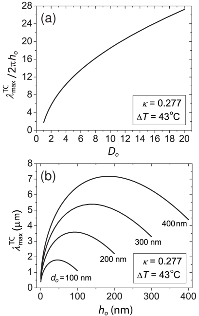
This expression provides an estimate of the average spacing between protrusions undergoing growth by thermocapillary flow. For the nanofilm experiments described earlier, $h_{o}\approx\textrm{O}~{}(100~{}\textrm{nm})$, $h_{o}<d_{o}\lesssim 8\>h_{o}$ and $\Delta T\approx 10-50\>^{\textrm{o}}\textrm{C}$. This leads to predictions of the pillar spacings ranging from about 2-20 $\mu$m. (More detailed comparison to experiments will be discussed in Section III.) According to Eq.  (27), the characteristic lateral spacing between nanopillars is determined by the initial film thickness, $h_{o}$, as well as the gap ratio $D_{o}=d_{o}/h_{o}$, the ratio of the surface tension to the maximum change in surface tension, $\gamma/(\gamma_{T}\Delta T)$, and the ratio of thermal conductivities $\kappa=k_{\textrm{air}}/k_{\textrm{melt}}$. For cases in which the geometry and material properties are held fixed, a larger thermal gradient produces more closely spaced pillars. Reversal of the thermal gradient such that $T_{2}<T_{1}$ should lead to linearly stable films.

Figure 2(a) represents solutions to Eq. (27) for a polystyrene film at $T_{2}=170^{\textrm{o}}$C with $\Delta T=43~{}^{\textrm{o}}$C. Smaller gap ratios $D_{o}$ lead to smaller values of pillar spacing since the film is subject to a larger effective thermal gradient. Figure 2(b) highlights the dependence of $\lambda^{\textrm{TC}}_{\textrm{max}}$ on the initial film thickness $h_{o}$ for various gap widths $d_{o}$ and $\Delta T=43^{\textrm{o}}$C. As evident, the prediction for $\lambda^{\textrm{TC}}_{\textrm{max}}$ depends sensitively on $h_{o}$, especially for the smallest values of $h_{o}$.

Figure 2: Solutions of Eq. (27) for $\kappa=0.277$ and $\Delta T=43^{\textrm{o}}\textrm{C}$. Curves show a sharp decrease in $\lambda^{\textrm{TC}}_{\textrm{max}}$ for the smaller values of $h_{o}$.

The linear stability analysis of Eq. (23) yields a prediction for the fastest growing wavelength for the acoustic phonon model, namely Eq. (1). The ratio of dominant wavelengths corresponding to the two proposed mechanisms is given by

$$\frac{\lambda^{\textrm{TC}}_{\textrm{max}}}{\lambda^{\textrm{AP}}_{\textrm{max}}}=\sqrt{\frac{4\,Q\,k_{\textrm{melt}}\,(1-\kappa)}{3\,u_{p}\,\gamma_{T}\,D_{o}}}.$$ (28)

Future experiments conducted with parallel substrates for a wider range of $D_{o}$ should help identify the operating mechanism leading to pillar formation.

The characteristic velocity defined earlier in Eq. (21), which sets the scale for the lateral flow speed based on thermocapillary stress, can be re-expressed in terms of the length scale $\lambda^{\textrm{TC}}_{\textrm{max}}$ obtained from linear stability analysis:

$$u_{\textrm{c}}=\epsilon\frac{(4\pi)^{2}}{3}\left(\frac{h_{o}}{\lambda^{\textrm{TC}}_{\textrm{max}}}\right)^{2}\frac{\gamma}{\eta}=\frac{(4\pi)^{2}}{3}~{}\epsilon^{3}\left(\frac{\gamma}{\eta}\right).$$ (29)

Here, the lateral scale $L$ used to define the slender gap parameter, $\epsilon=h_{o}/L$, is identified with $\lambda^{\textrm{TC}}_{\textrm{max}}$. Similarly, the characteristic timescale based on thermocapillary flow is given by

$$t_{\textrm{c}}=\frac{\lambda^{\textrm{TC}}_{\textrm{max}}}{u_{\textrm{c}}}=\frac{3h_{o}}{(4\pi)^{2}\epsilon^{4}}\left(\frac{\eta}{\gamma}\right).$$ (30)

Estimates from the experiments of Schäffer et al. indicate that $u_{\textrm{c}}$ is of the order of $10^{-1}-10^{1}$ nm/s and $t_{\textrm{c}}\approx\textrm{O}(10^{-1}-10^{2}\>\textrm{hrs})$. If the thermocapillary flow speed $u_{\textrm{c}}$ given by Eq. (29) is used to define the capillary number, then $\overline{Ca}=(4\pi)^{2}/3$, a fixed constant. Replacing the capillary number by this numerical value and substituting the expression for the Marangoni number given by Eq. (20) into the interface equation Eq. (19) yields the following form of the evolution equation:

$$\frac{\partial H}{\partial\tau}+\nabla_{\parallel}\cdot\left\{\left[\frac{D_{o}\!+\kappa\!-\!1}{D_{o}\!+\!(\kappa\!-\!1)H}\right]^{2}\!\frac{H^{2}}{2}\nabla_{\parallel}H+\frac{H^{3}}{(4\pi)^{2}}\nabla^{3}_{\parallel}H\right\}=0.$$ (31)

For thicker films, hydrostatic forces can be re-incorporated into this expression by including the term $-\overline{Bo}\>H^{3}\nabla_{\parallel}H/(4\pi)^{2}$ in the curly brackets. During the early stages of film deformation when $H$ and $\nabla_{\parallel}H$ are order one, the relative magnitude of terms in Eq. (31) reveals the basis for pillar formation. The ratio of thermocapillary to capillary flux scales as $8\pi^{2}$, while the ratio of thermocapillary to gravitational flux scales as $8\pi^{2}/\overline{Bo}\approx 10^{7}-10^{8}$. These estimates reveal that thermocapillary forces overcome the stabilizing effect of capillary and gravitational forces even at early times. In section IV.B, it is shown that thermocapillary forces prevail even more strongly at late times for parameter values pertinent to the nanofilm experiments. A similar comparison can be made using the parameter values in the experiments of VanHook et al. VanHook (1996) with thicker films ($70\lesssim h_{o}\lesssim 270\>\mu\textrm{m}$) and much smaller transverse thermal gradients ($180\lesssim T_{2}-T_{1}/d_{o}\lesssim 500$ ${}^{\textrm{o}}$C/cm). While the thermocapillary to capillary flux ratio remains at $8\pi^{2}$, the thermocapillary to gravitational flux ratio decreases to $10^{-1}$, eight to nine orders of magnitude smaller than the ratio in the nanofilm experiments of Sch$\ddot{a}$ffer et al. and Peng et al. . While gravitational forces effectively repress the growth of pillars in macroscopically thick films, this order of magnitude analysis confirms that hydrostatic forces are ineffective in repressing the growth of elongations in nanoscale films.

Integration of the full nonlinear Eq. (19) can be used to compute a lower bound on the time interval, $t_{\textrm{top}}$, required for nanopillars to contact the cooler substrate within the approximation of a constant film viscosity foo . It will be shown in Section IV.A that estimates obtained from the growth rate of the most unstable mode, $\beta(K_{\textrm{max}})$, are in fairly good agreement with the estimates obtained from numerical solutions of Eq. (19) for the parameter range of interest. Substitution of Eq. (20) and $\overline{Ca}=(4\pi)^{2}/3$ into Eq. (24) and Eq. (25) yields the simplified expression for the growth rate:

$$\beta^{\textrm{TC}}(K)=[1/2-(K/(4\pi))^{2}]K^{2}.$$ (32)

The wave number corresponding to marginal stability is therefore $K^{\textrm{TC}}_{\textrm{M}}=4\pi/\sqrt{2}$. Since $K^{\textrm{TC}}_{\textrm{max}}=K^{\textrm{TC}}_{\textrm{M}}/\sqrt{2}=2\pi$, the growth rate for the fastest growing mode simply reduces to $\beta^{\textrm{TC}}_{\textrm{max}}=\pi^{2}$. Setting $\widetilde{\delta H_{o}}\exp[\beta(K_{\textrm{max}})\tau]=D_{o}-1$ leads to the expression $\tau_{\textrm{top}}=\ln[(D_{o}-1)/\widetilde{\delta H_{o}}/\pi^{2}$, which in dimensional units corresponds to $t_{\textrm{top}}=(3\>\eta\>h_{o}/\gamma)[\lambda^{\textrm{TC}}_{\textrm{max}}/(2\pi h_{o})]^{4}\ln[(D_{o}-1)/\widetilde{\delta H_{o}}]$. Substitution of Eq. (27) into this expression then gives

$$t_{\textrm{top}}=\frac{16\>\eta\>\gamma\>h_{o}(D_{o}+\kappa-1)^{4}}{3\>(\kappa\>D_{o}\>\gamma_{T}\>\Delta T)^{2}}\ln\left(\frac{D_{o}-1}{\widetilde{\delta H_{o}}}\right).$$ (33)

Estimates of $t_{\textrm{top}}$ for the nanopillar experiments range from about tens of minutes to tens of hours for the largest gap spacings used and $\widetilde{\delta H_{o}}=10^{-5}$. Low molecular weight polymers with much smaller viscosities require proportionally less time to contact the cooler top substrate. Studies of this sort are useful in determining when to remove the thermal gradient in order to form nanopillars of specified height.

II.1.2 Lyapunov free energy for evolving interface

Hydrodynamic systems subject to interfacial instability sometimes exhibit steady states as observed in Rayleigh-Bénard or Bénard-Marangoni cellular convection. Within the context of the experiments described, this would require pillar formations which once formed, neither grow nor decay, representing a fixed spatial configuration while the melt continues to undergo surface and interior flow. To examine this possibility, one can investigate the temporal behavior of the Lyapunov free energy associated with the evolving interface, as previously implemented in Refs. [46, 47]. This approach is based on the analysis of interface problems using the well known form of the Cahn-Hilliard free energy for systems with spatial variation in an intensive scalar variable like composition or density Cahn and Hilliard (1958). The Cahn-Hilliard equation has been successfully used to explore the evolution of moving interfaces in binary systems undergoing phase separation. This approach, which involves monitoring the free energy associated with the entire film undergoing deformation, provides a more accurate assessment of possible steady state configurations than simple considerations based on Eq.(31) in the limit $\partial H/\partial\tau\rightarrow 0$.

In the Appendix, it is shown that the free energy corresponding to the nanofilms of interest is given by $\mathfrak{F}=\int\mathfrak{L}~{}dXdY$, where

$$\mathfrak{L}\!=\!(\nabla_{\parallel}H)^{2}\!-\!\frac{3\kappa\overline{Ma}\>\overline{Ca}}{D_{o}}\left[H\textrm{ln}\left(\frac{H}{1+\chi H}\right)\!+\!\textrm{ln}(1+\chi)\right]$$ (34)

and $\chi=(\kappa-1)/D_{o}$. Numerical solutions of Eq. (A-13) for large and small values of the gap ratio, $D_{o}$, are discussed in Section IV.B.

II.2 Films confined by non-parallel substrates

The analysis presented in Section II.A describes the evolution of a fluid bilayer interface confined by two flat and parallel substrates separated by a distance $D_{o}=d_{o}/h_{o}$. As described in Section I.A.2, however, Schäffer and co-workers purposely used in all their experiments a tilted plate geometry in which the top wafer was inclined with respect to the bottom one by about $1\mu\textrm{m}/1\textrm{cm}$, corresponding to an inclination angle $\varphi$ of about $0.0057^{\textrm{o}}$. The evolution equation can be modified to account for two flat substrates with relative tilt. When the cooler substrate is tilted away from the horizontal by a constant angle $\varphi$, the local value of the plate separation will depend on $(X,Y)$ such that $D(X,Y)=d(x,y)/h_{o}$. This modification alters the film surface temperature, $\Theta|_{Z=H}$, as well as the surface thermal gradient, $\nabla\Theta|_{Z=H}$, which in turn alters the interfacial thermocapillary stress, $\nabla_{\parallel}\Gamma$. Accordingly,

$$\Theta|_{Z=H}=(D-H)/[D+(\kappa-1)H]~{},$$ (35)

$$\nabla_{\parallel}\Theta|_{Z=H}=\frac{\kappa}{[D+(\kappa-1)H]^{2}}\left(H\nabla_{\parallel}D-D\nabla_{\parallel}H\right),$$ (36)

and

$$\nabla_{\parallel}\Gamma|_{Z=H} = -\overline{Ma}\nabla_{\parallel}\Theta|_{Z=H}$$ (37)

$$= \kappa\overline{Ma}~{}\frac{\left(D\nabla_{\parallel}H-H\tan(\overline{\varphi})\overrightarrow{T}_{\parallel}\right)}{[D+(\kappa-1)H]^{2}}.$$

Here, $D(\overrightarrow{X}_{\parallel})=D_{o}+\tan(\overline{\varphi})\overrightarrow{T}_{\parallel}\cdot\overrightarrow{X}_{\parallel}$, where $D_{o}$ represents the gap ratio at $\overrightarrow{X}_{\parallel}=0$ (later identified with the midpoint of the computational domain). The quantities $\overline{\varphi}$ and $\tan\overline{\varphi}=\tan\varphi/\epsilon$ represent variables rescaled according to the slender gap approximation. In the numerical solutions discussed in Section IV.C.2, the tilt of the upper substrate is defined by the unit vector $\overrightarrow{T}_{\parallel}=(1,1)/\sqrt{2}$. Substitution of Eq. (37) into Eq. (16) and Eq. (14) leads to the modified evolution equation

$$\frac{\partial H}{\partial\tau}+\nabla_{\parallel}\cdot\vec{Q}_{\textrm{tilt}}=0~{},$$ (38)

where

$$\vec{Q}_{\textrm{tilt}}=\frac{\kappa\overline{Ma}H^{2}(D\nabla_{\parallel}H-H\tan(\overline{\varphi})\overrightarrow{T}_{\parallel})}{2[D+(\kappa-1)H]^{2}}+\frac{H^{3}}{3\overline{Ca}}\nabla^{3}_{\parallel}H.$$ (39)

A linear stability analysis of Eq. (38) (not shown here) confirms that the pattern wavelength in Eq. (27) remains unaffected by the small tilt angle used in the experiments of Schäffer et al. . More generally, Eq. (27) remains valid so long as $|\tan(\overline{\varphi})|\leq\textrm{O}(\widetilde{\delta H_{o}})$.

III Nanopillar Spacings: Comparison Between Experiment and Theory

Shown in Fig. 3(a) is a direct comparison of Eq. (27) with the experimental data of Schäffer et al. Schäffer et al. (2002, 2003a) The solid lines denote the predictions of the thermocapillary model with no adjustable parameter values using the material properties listed in Table 2; the symbols denote the experimental data.

Figure 3: Direct comparison of theoretical estimates for dominant instability wavelength, $\lambda_{\textrm{max}}$ for both thermocapillary (TC) and acoustic phonon (AP) models with experimental measurements from Schäffer et al. Schäffer et al. (2002, 2003a, 2003b); Schäffer (2001) as function of increasing wafer separation distance $d_{o}$. (a) Plots of Eq. (27) for thermocapillary model with no adjustable parameters for different experiments labeled A-D using material constants listed in Table 2. (b) Plots showing least squares fits to the TC and AP models. The TC model was fitted to the form given by Eq. (27), namely $\lambda^{\textrm{TC}}_{\textrm{max}}=C_{1}\sqrt{d_{o}}+C_{2}/\sqrt{d_{o}}$. AP model was fitted to the function given by Eq. (1) with $u_{p}=1850\>\textrm{m/s}$ and $Q=6.2$ as fitting parameters. Table 3 lists the fitting coefficients, $C_{1}$ and $C_{2}$, obtained for the TC model.

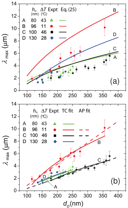
While the overall functional behavior of $\lambda^{\textrm{TC}}_{\textrm{max}}$ with $d_{o}$ is in good agreement with experiment, the model systematically overestimates the pillar spacings, in some cases by as much as $40\%$. This is especially evident in experimental run B for which $h_{o}=96$ nm and $\Delta T=11\>^{\textrm{o}}\textrm{C}$. Before discussing these discrepancies in detail, it is useful to examine a least-squares fit of the data to the function $\lambda^{\textrm{TC}}_{\textrm{max}}=C_{1}\>{d_{o}}^{1/2}+C_{2}\>{d_{o}}^{-1/2}$ given by Eq. (27), as shown in Fig. 3(b). Listed in Table 3 is a comparison of the analytic expressions for the two constants, namely $C^{\textrm{TC}}_{1}=2\pi[{4\>h_{o}\>\gamma/(3\>\kappa\>\gamma_{T}\>\Delta T]^{1/2}}$ and $C^{\textrm{TC}}_{2}=C_{1}\>(\kappa-1)\>h_{o}$, along with the results for the fitting constants denoted by $C^{\textrm{Fit}}$.

Table 3: Coefficients obtained from a least squares fit to the data of Schäffer et al. [22, 26]. Experimental data were fit to the function $\lambda^{\textrm{TC}}_{\textrm{max}}=C_{1}\>{d_{o}}^{1/2}+C_{2}\>{d_{o}}^{-1/2}$ given by Eq. (27), where $\lambda^{\textrm{TC}}_{\textrm{max}}$ is reported in microns and $h_{o}$ and $d_{o}$ in nm. The constants $C^{\textrm{Fit}}$ denote the values obtained for the least squares fits shown in Fig. 3. The constants $C^{\textrm{TC}}$ represent the predictions of the TC model given by Eq. (27) with no adjustable parameters using the material properties listed in Table 2. The percentage errors are defined by $(C^{\textrm{Fit}}-~{}C^{\textrm{TC}})/C^{\textrm{TC}}$.

		A	B	C	D
	$h_{o}~{}~{}~{}(\textrm{nm})$	80	96	100	130
	$\Delta T~{}~{}~{}(^{\textrm{o}}\textrm{C})$	43	11	46	28
$C^{\textrm{TC}}_{1}$	[$(10^{3}\>\mu\textrm{m})^{0.5}$]	0.36	0.77	0.38	0.56
$C^{\textrm{TC}}_{2}$	[$(10^{-1}\>\mu\textrm{m})^{1.5}$]	-21	-53	-28	-53
$C^{\textrm{Fit}}_{1}$	[$(10^{3}\>\mu\textrm{m})^{0.5}$]	0.35	0.65	0.38	0.34
		$\pm$	$\pm$	$\pm$	$\pm$
		0.036	0.058	0.031	0.071
$C^{\textrm{Fit}}_{2}$	[$(10^{-1}\>\mu\textrm{m})^{1.5}$]	-35	-65	-46	-31
		$\pm$	$\pm$	$\pm$	$\pm$
		7.5	12	8.7	13
$\%$ Error $C_{1}$		-0.53	16	1.2	39
$\%$ Error $C_{2}$		-69	-21	-66	42

In general, the agreement between the TC model and experiment improves for larger values of $\Delta T$. However, given that the least squares fit captures the experimental trend with increasing values of $h_{o}$ and $d_{o}$ so well, it is worth considering what experimental challenges might affect the reported measurements. For completeness, we include in Fig. 3(b) two additional dashed lines for runs B and C, which represent a least squares fit of the data to Eq. (1) with $Q=6.2$ and $u_{p}$ = 1850 m/s, the same fitting constants reported by Schäffer et al. Schäffer et al. (2002, 2003a)

III.1 Possible causes of discrepancy between theory and experiment

There are several experimental challenges in performing the experiments on nanopillar formation. Perhaps the most important is that all experiments to date have used silicon wafers to confine the polymer films. These opaque substrates prevent observation of the instability in-situ. In fact, measurements of the pillar spacings were normally obtained long after the pillars had contacted the cooler wafer. The pillar amplitudes were by then sizeable, possibly violating the assumptions of linear stability analysis. Furthermore, the warmer nanopillars had sustained prolonged contact with a cooler substrate leading to possible reorganization of fluid due to thermocapillary or other packing effects along the underside of the top wafer. Measurements taken once the pillars had solidified and the top wafer was removed may therefore differ from the predictions of linear stability theory. In many of the experiments described earlier, measurements of the spacing between fluid elongations included not only pillar arrays, but lamellar, spiral and other periodic structures since these were more commonly obtained. An additional complication is that a typical molten nanofilm is not completely smooth and flat due to the presence of contaminant particles and pinholes caused by dewetting. Any small fluid elevations caused by these nucleation points are prone to rapid growth when subject to a thermal gradient. Structures arising from such initial conditions, however, correspond more to disturbances of finite amplitude and not infinitesimal amplitudes as assumed by the linear analysis.

As evident from the curves in Fig.  2, the parameters $h_{o}$ and $d_{o}$ strongly affect the predicted values of $\lambda^{\textrm{TC}}_{\textrm{max}}$. The sharp drop in $\lambda^{\textrm{TC}}_{\textrm{max}}$ becomes even more pronounced for smaller values of $\Delta T$ Dietzel and Troian (2009). Validation of either mechanism proposed therefore requires accurate measurements of the film thickness. It appears that the films used by Schäffer et al. Schäffer (2001); Schäffer et al. (2002, 2003a, 2003b) and Peng et al. Peng et al. (2004) were not annealed prior to insertion in the experimental setup. Spun cast polymer films tend to retain a significant amount of solvent García-Turiel and Jérôme (2007); Perlich et al. (2009), which is normally expelled by film annealing in vacuum at elevated temperatures for several hours. (Annealing has the additional advantage of healing pin holes that sometimes form during spin coating.) Significant film shrinkage typically accompanies this process due to solvent evaporation. The degree of film shrinkage depends on the ambient vapor pressure as well as the time and temperature of the bake. It is therefore likely that the values of $h_{o}$ reported in the literature represent overestimates of the initial film thickness $h_{o}$. Smaller values of $h_{o}$ lead to smaller predictions for the pillar spacing, in closer agreement with experiment.

The distance between pillars in experiment was typically obtained by direct measurement from optical micrographs. In future experiments, it would be preferable to Fourier analyze the patterns obtained by an FFT (Fast Fourier Transform) analysis. This analysis may reveal not only the dominant wave number but harmonics that develop due to the growth of smaller pillars in between two larger neighboring ones. Such an analysis, however, requires a fair number of protrusions for statistically meaningful results. It may have been the case with the tilted plate geometry, that the smaller domains corresponding to each distinct value of $D_{o}$ forbade use of this technique.

We conducted FFT analyses of nanopillar arrays published in the literature Schäffer (2001); Schäffer et al. (2002, 2003a) and were surprised to find a very wide distribution in pillar spacings within even a single experiment. Often there appeared not a single dominant wavelength but several competing wavelengths. This finding prompted a sensitivity analysis of Eq. (27) to better understand which variables most strongly affect the uncertainty in measurements of $\lambda^{\textrm{TC}}_{\textrm{max}}=\lambda^{\textrm{TC}}_{\textrm{max}}(\xi_{i})$, as defined by $U_{\lambda^{\textrm{TC}}_{\textsf{max}}}=\sqrt{\sum_{i}(S_{\xi_{i}}\>\Delta\xi_{i}/\xi_{i})^{2}}$. Here, the relative sensitivity coefficients are given by $S_{\xi_{i}}\!=\!\xi_{i}\>\partial\lambda^{\textrm{TC}}_{\max}/\partial\xi_{i}$ where $\xi_{i}=(\gamma,\>\gamma_{T},\>\Delta T,\>\kappa,\>D_{o},\>h_{o})$. This analysis demonstrates that $S_{\gamma}=-S_{\gamma_{T}}=-S_{\Delta T}=1/2\>\lambda^{\textrm{TC}}_{\textrm{max}}$, $S_{\kappa}=[\kappa/(D_{o}+\kappa-1)-1/2]\lambda^{\textrm{TC}}_{\textrm{max}}$, $S_{D_{o}}=[D_{o}/(D_{o}+\kappa-1)-1/2]\lambda^{\textrm{TC}}_{\textrm{max}}$ and $S_{h_{o}}=[1/2+(\kappa-1)/(D_{o}+\kappa-1)]\lambda^{\textrm{TC}}_{\textrm{max}}$. Typical values for these sensitivity coefficients for the parameter values corresponding to the experiments of Schäffer et al. are summarized in Table 4. These values indicate that the gap ratio, $D_{o}=d_{o}/h_{o}$, the initial film thickness, $h_{o}$, and the polymer surface tension, $\gamma$, most significantly influence the degree of uncertainty in measurements of $\lambda^{\textrm{TC}}_{\textrm{max}}$.

Table 4: Typical values of sensitivity coefficients $S_{\xi_{i}}/\lambda^{\textrm{TC}}_{\textrm{max}}$ resulting from Eq. (27)
where $\xi_{i}=\gamma,\>\gamma_{T},\>\Delta T,\>\kappa,\>D_{o}~{}\textrm{or}~{}h_{o}$.

$S_{\gamma}/\lambda^{\textrm{TC}}_{\textrm{max}}$	0.5
$S_{\gamma_{T}}/\lambda^{\textrm{TC}}_{\textrm{max}},\>S_{\Delta T}/\lambda^{\textrm{TC}}_{\textrm{max}}$	-0.5
$S_{\kappa}/\lambda^{\textrm{TC}}_{\textrm{max}}$	-0.5 to -0.25
$S_{D_{o}}/\lambda^{\textrm{TC}}_{\textrm{max}}$	0.6 to 1.1
$S_{h_{o}}/\lambda^{\textrm{TC}}_{\textrm{max}}$	0 to 0.4

IV Numerical simulation of thin film equation: linear and non-linear regimes

To investigate the extent of non-linear effects on the growth of nanopillars, we also conducted 3D finite element simulations of Eq. (19) using a commercial software package COM . Material properties corresponding to molten polystyrene (PS) were used in these numerical studies (see Table 2). The computational domain corresponded to a square of size $\Delta X\times\Delta Y=6\lambda^{\textrm{TC}}_{\textrm{max}}\times 6\lambda^{\textrm{TC}}_{\textrm{max}}$ (according to Eq. (27)) where spatial discretization was obtained via second order Lagrangian shape functions. This choice in domain size and discretization order reflects a compromise between available computational resources and generation of a sufficient number of peaks for FFT analysis. Periodic boundary conditions were enforced along the domain edges (except for the simulations using tilted substrates). A quadrilateral mesh consisting of $200\times 200$ elements was applied for the coarse (non-extended) discretization, leading to an extended system of equations with about $5\cdot 10^{5}$ degrees of freedom. An implicit Newton iteration scheme was used to advance the position of the film interface in time; the linear system of equations for each iteration was solved using the iterative solver GMRES (Generalized Minimal Residual Method). All simulations were conducted on HP ProLiant DL360 G4p workstations equipped with dual Intel Xeon 3.0 GHz processors running CentOS 4.6. The typical growth of a nanopillar spanning two substrates (i.e. $\tau=\tau_{\textrm{top}}$) required approximately $5-6\>\textrm{hrs}$ of CPU time, corresponding to about 900-1000 integration steps. Numerical convergence tests were conducted by evaluating the local dimensionless film height at $N=400$ interpolation points within the square domain. These tests confirmed that both the average difference, $\Delta H_{\textrm{avg}}=\sum^{N}_{i=1}|H_{2}(X,Y,\tau_{\textrm{top})}-H_{1}(X,Y,\tau_{\textrm{top})}|/N$, as well as the maximum difference, $\Delta H_{\textrm{max}}=\max|H_{2}(X,Y,\tau_{\textrm{top}})-H_{1}(X,Y,\tau_{\textrm{top}})|/N$, in film height at the end of a run (i.e. $\tau=\tau_{\textrm{top}}$) were less than $10^{-4}$ when decreasing the grid size or integration time step. Here, $H_{1}$ denotes the coarser measurement and $H_{2}$ the refined one. Further tests revealed that the film volume was conserved during each run to a value $\Delta V/V=|\int[H(X,Y,\tau_{\textrm{top}})-H(X,Y,\tau=0)]~{}dXdY|/(\Delta X\Delta Y)\leq 10^{-10}$.

In all simulations conducted, the thickness of the initial flat film was modulated by a very small amount of white noise such that $H(X,Y,\tau=0)=1+\xi\>\mathfrak{R}$, where $\mathfrak{R}$ denotes a random number between $-1$ and $+1$. The amplitude of the white noise was set to $\xi=\textrm{O}(10^{-5})$. According to Eq. (33), larger values of $\xi$ will lead to shorter contact times in proportion to $-\ln({\widetilde{\delta H_{o}}})$. In order to facilitate detailed comparison between runs for different choices of experimental parameters, the random number algorithm was reset before each run so as to generate an identical white noise distribution. Initialization with white noise was preferable to initialization by a sinusoidal function, as is common, in order not to bias the system toward a preferred wavelength too early in the pillar formation process.

IV.1 Films confined by parallel wafers

FFTs of the in-plane images obtained from the numerical solution of Eq. (19) were used to extract values of the dominant wavelength, $\lambda^{\textrm{simul}}_{\textrm{max}}(\tau)$, at each instant in time. This numerical value was compared to the theoretical prediction $\lambda^{\textrm{TC}}_{\textrm{max}}$ given by Eq. (27). Shown in Fig. 4 are results of these simulations.

Figure 4: Direct comparison of $\lambda^{\textrm{TC}}_{\textrm{max}}$ from Eq. (27) with the instantaneous wavelength, $\lambda^{\textrm{simul}}_{\textrm{max}}$, extracted from FFT analysis of numerical solutions of the evolving film thickness from Eq. (19) with increasing dimensionless time $\tau$. Symbol $\tau_{\textrm{top}}$ represents time of contact of the fastest growing pillar with cooler substrate. Times $\tau_{o}=0$, $\tau_{1}=0.06$ and $\tau_{\textrm{top}}=1.23$ shown in the top panel refer to time stamps of the snapshot images shown next in Fig. 5. (a) Variation of the wavelength ratio with increasing temperature difference $\Delta T$. (b) Variation of the wavelength ratio with increasing gap separation distance $d_{o}$. (c) Variation of the wavelength ratio with increasing values of initial film thickness $h_{o}$.

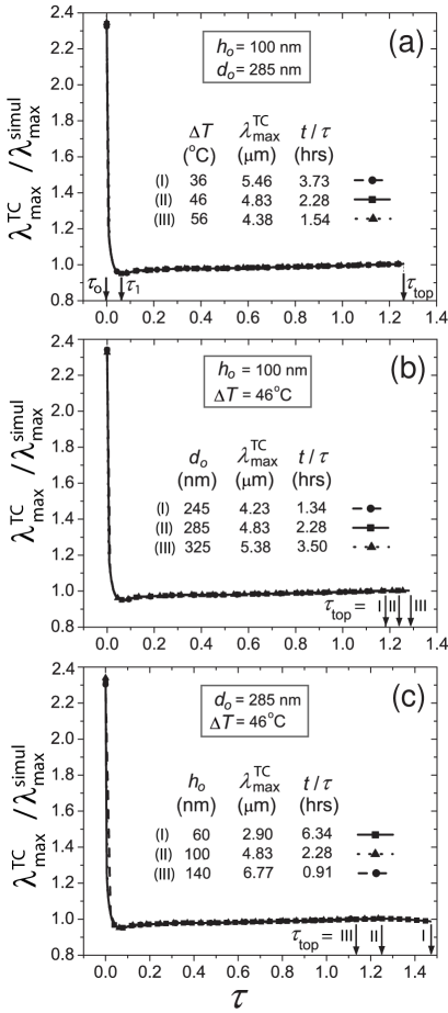
The FFTs were computed by sampling $200\times 200$ points within the computational domain for each value of $\tau$; approximately 140 instances in time were so evaluated. The legend in each plot represents the variables held fixed during the simulation; the table entries specify the theoretical values of $\lambda^{\textrm{TC}}_{\textrm{max}}$ corresponding to the chosen parameter set. For convenience, the factor used in converting $\tau$ to real time $t$ is also listed. The times $\tau_{o}=0$, $\tau_{1}=0.06$ and $\tau_{\textrm{top}}=1.23$ shown in Fig. 4(a) denote the three instances in time for for which the FFTs shown in Fig.  5 were computed. The variable $\tau_{\textrm{top}}$ denotes the time at which the fastest growing nanopillar in a particular run made contact with the cooler substrate, at which point the simulation is terminated. The times $\tau_{\textrm{top}}=\textsf{I, II or III}$ indicate this contact time for the parameters values designated by (I), (II) or (III).

As evident, the overall deviation of $\lambda^{\textrm{simul}}_{\textrm{max}}(\tau)$ from $\lambda^{\textrm{TC}}_{\textrm{max}}$ is rather small regardless of the parameter range used. In all cases, this ratio rapidly approaches unity as $\tau\rightarrow 1$. The only discernible difference is that the fastest growing peaks require a longer time to contact the cooler substrate for larger values of the relative gap spacing $D_{o}=d_{o}/h_{o}$, as expected. The very short lived but large initial transients are caused by initialization with white noise; shortly following $\tau=0$, there exist disturbances of all wavelengths. Those contributions with wave number larger than the cut-off wave number $K_{\textrm{c}}$ become rapidly damped. The ratio $\lambda^{\textrm{simul}}_{\textrm{max}}(\tau)/\lambda^{\textrm{TC}}_{\textrm{max}}$ then drops sharply to a value close to one as the maximally unstable disturbance is established. The approach to unity from below rather than above is due to the asymmetry in the dispersion curve $\beta(K)$ for which there exists a broader band of unstable wave numbers below $K_{\textrm{max}}$ than above.

Additional simulations (not shown for brevity) reveal that $\lambda^{\textrm{simul}}_{\textrm{max}}/\lambda^{\textrm{TC}}_{\textrm{max}}\rightarrow 1$ by $\tau=1$ irrespective of the specific initialization function used i.e. white noise or a simple sinusoidal function. Initialization by a double cosine wave in $(X,Y)$ with wavelength $\lambda_{\textrm{c}}=\lambda^{\textrm{TC}}_{\textrm{max}}/\sqrt{2}$, for example, produced the same long time behavior shown so long as the amplitude of the disturbance function satisfied $\widehat{\delta H_{o}}\ll 1$.

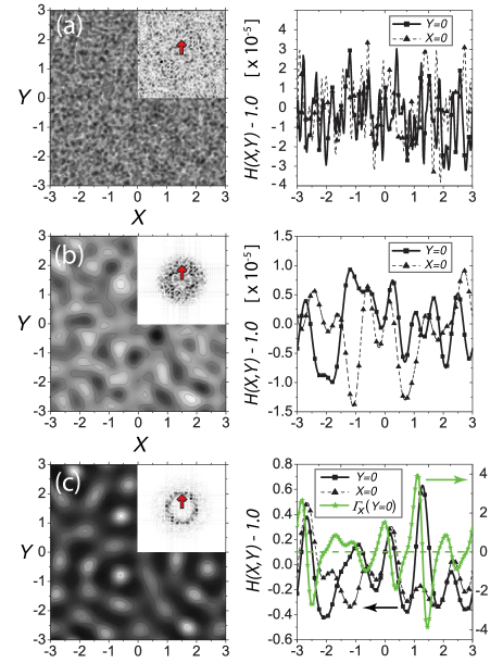
Images of the evolving film thickness, $H(X,Y,\tau)-1$, as seen from above, the corresponding Fourier transform (insets), and cross-sectional views along the mirror planes $X=0$ and $Y=0$ are shown in Fig. 5 at times $\tau=0,\>0.06~{}\textrm{and}\>1.23$. The relevant parameters values are $h_{o}=100\>\textrm{nm}$, $d_{o}=285\>\textrm{nm}$ and $\Delta T=46\>^{\textrm{o}}\!\textrm{C}$, which represent case II) in Fig. 4]. The arrow shown in the FFT with unit length denotes the magnitude $K^{\textrm{TC}}_{\textrm{max}}$. As evident from the images in Figs. 5(a) and (b), although the disturbance heights of order $10^{-5}$ do not increase substantially from $\tau=0$ to 0.06, an increasingly regular hexagonal pattern is already visible, both in the Fourier transform as well the cross sectional views. Figure 5(c) depicts the in-plane symmetry in a fully evolved film, just as the fastest growing peak contacts the cooler substrate. Here, the pillar amplitudes have increased substantially in comparison to their initial values. By this time, the Fourier transform of the emerging pattern has evolved from a wide band into a narrow ring with distinct six-fold symmetry and mean radius $K^{\textrm{TC}}_{\textrm{max}}$. Values of the (dimensionless) interfacial shear stress, $\Gamma_{X}=\partial\Gamma/\partial X$, along the axis $Y=0$ for $\tau=1.23$ are shown in the bottom right image. As expected from symmetry, the local extrema in film thickness along $Y=0$ (solid black curve) occur at the locations of vanishing shear stress i.e. $\Gamma_{X}=0$. The largest values of $|\Gamma_{X}|$ tend to occur near the maxima and minima in film thickness.

Figure 5: View from above of numerical solutions of the film thickness, $H(X,Y,\tau)-1.0$ from Eq. (19) at three instants in time: (a) $\tau_{0}=0$ (origin of time), (b) $\tau_{1}=0.06$ and $\tau_{\textrm{top}}=1.23$. Simulation parameters values are $h_{o}$= 100 nm, $d_{o}$=285 nm and $\Delta T=46^{\textrm{o}}\textrm{C}$. Evolution of the corresponding dominant wavelength is depicted by case (II) in Fig. 4(a). Left panel depicts amplitude $H(X,Y,\tau)-1.0$ (white = elevations, black = depressions); right panel depicts cross sectional views along axes $X=0$ and $Y=0$. Inset images show the instantaneous 2D Fourier transform of the corresponding film thickness. Unit arrows denote magnitude of most unstable wave number, $K^{\textrm{TC}}_{\textrm{max}}/\sqrt{2}=2\pi$, derived from linear stability theory [see discussion following Eq. (32)]. Values of the dimensionless interfacial shear stress, $\Gamma_{X}=\partial\Gamma/\partial X$, along the axis $Y=0$ are shown in the bottom right image.

Shown in Fig. 6 is the growth rate ratio, $\beta^{\textrm{simul}}_{\textrm{max}}/\beta^{\textrm{TC}}_{\textrm{max}}$, for the parameter values labeled (b) in Fig. 4 and Fig. 5. This ratio was computed for each of the six most rapidly growing peaks according to

$$\frac{\beta^{\textrm{simul}}_{\textrm{max}}}{\beta^{\textrm{TC}}_{\textrm{max}}}=\frac{3\>\eta\>h_{o}}{\gamma}\left(\frac{\lambda^{\textrm{TC}}_{\textrm{max}}}{2\pi_{o}}\right)^{4}\frac{1}{\delta h_{o}}\frac{\partial(\delta h_{o})}{\partial t}.$$ (40)

Here, $\beta^{\textrm{TC}}_{\textrm{max}}=\pi^{2}$, as shown in Section II.A.1.

Figure 6: Direct comparison of instability growth rate, $\beta^{\textrm{TC}}_{\textrm{max}}=\pi^{2}$ (as discussed in Section II.A.1), with instantaneous growth rate, $\beta^{\textrm{simul}}_{\textrm{max}}$, from Eq. (40), with increasing time $\tau$. Different curves shown correspond to growth rates of six fastest peaks for parameter values $h_{o}\!=\!100$ nm, $d_{o}\!=\!285$ nm and $\Delta T\!=\!46\>^{\textrm{o}}\textrm{C}$. Inset image depicts film shape for $H(X,Y,\tau_{\textrm{top}}=1.23)$.

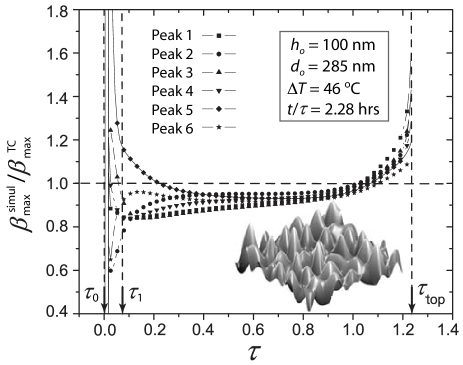
As in the solutions shown in Fig. 4, here too the numerical results are initially influenced by the white noise disturbance spectrum. Each of the six fastest growing peaks behaves somewhat differently at the earliest times depending on what is the local value of the disturbance height. However, the growth rates collapse rapidly by about $\tau=0.4$, after which the average growth rate slowly increases toward the prediction of linear stability theory, which is established by about $\tau=1.0$. Beyond this time, the solutions reveal rapid growth and an increasing departure from the predictions of linear stability theory as nonlinear effects contribute to the evolving pattern. Beyond $\tau\approx 1.0$, the growing nanopillars are within reach of the cooler substrate. The instances marked $\tau_{0}$, $\tau_{1}$ and $\tau_{\textrm{top}}$ represent exactly those times indicated in Fig. 4(a) and Fig. 5.

IV.2 Numerical simulations of Lyapunov free energy

Numerical solutions of Eq. (19) confirm that nonlinear effects for the parameter sets examined become signficant only when fluid elongations come into close proximity with the cooler substrate. As evident in Fig. 6, the elongation rate then exceeds exponential growth. In this regime, the nanopillars have grown a distance large in comparison to the initial film disturbance heights and the nonlinear terms in Eq. (19) strongly influence the flow. To explore the energetics of formation beyond the linear regime, we investigated the temporal behavior of the Lyapunov free energy given by Eq. (34). Shown in Fig. 7 are solutions of the free energy $\mathfrak{F}=\int\mathfrak{L}~{}dXdY$ for a polystyrene nanofilm with $h_{o}=100\>\textrm{nm}$ and $\Delta T=46^{\textrm{o}}\!\textrm{C}$ for two different wafer separation distances, $d_{o}=285$ nm and 800 nm. The termination points represent $\tau_{\textrm{top}}$. The individual contributions to the total free energy (denoted by “Sum”) from capillary and thermocapillary terms feature several important points.

Figure 7: Numerical solutions of Lyapunov free energy, $\mathfrak{F}(\tau)$, for an initial flat film of thickness $h_{o}=100$ nm and temperature difference $\Delta T=46^{\textrm{o}}\textrm{C}$ subject to two wafer separation distances: (a) $d_{o}$ = 285 nm and (b) 800 nm.

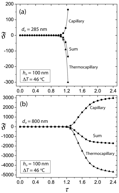
For $\tau\lesssim 1$, the film experiences small deformations such that the opposing capillary and thermocapillary contributions are also small, neither significantly enhancing nor depleting energy from the evolving film. Magnified views of the curves (not shown) confirm a small but monotically decreasing value of the free energy due to the still dominant influence of thermocapillary stresses. This period of growth corresponds to the linear regime described by linear stability analysis. Strong departure from this behavior occurs for $\tau\gtrsim 1$ when nonlinear effects begin to dominate. In this regime, the time (or distance) remaining for fluid contact with the top wafer is small and the energetics of pillar formation strongly affected by the presence of the cooler target. For the smaller gap separation distance ($d_{o}$ = 285 nm) shown Fig.7 (a), thermocapillary effects dominate capillary effects as the nanopillars grow ever more rapidly toward the cooler target. There remains sufficient fluid in the residual film to continue feeding the growth of nanopillars such that the system continuously lowers its overall free energy by transporting fluid toward the cooler substrate. Unlike the equilibrium cellular convective patterns observed with Rayleigh-Bénard or Bénard-Marangoni instabilities, this nanofilm instability is non-saturating and the free energy continues to decrease until the fluid makes contact with the cooler target.

The results shown in Fig. 7(b) for the larger gap separation distance $d_{o}=800$ nm reveal different behavior. Since the top substrate is positioned further away, the initial thermal gradient is smaller and the films require correspondingly longer times to develop substantial fluid elongations. The linear to nonlinear transition is observed to occur at slightly later times, $\tau\approx 1.2$. The individual contributions to the free energy are still clearly distinguishable but eventually asymptote. The larger wafer separation distance allows for longer growth periods, which causes significant film depletion near the base of nanopillars. Fluid transfer needed to grow the elongations is impeded, eventually halting their growth. Fluid already contained within the nanopillars continues to undergo a circulatory flow pattern, rising upwards near the surface due to thermocapillary stresses and falling downwards near the interior due to capillary stresses. However, fluid transfer from the initial deposited film slows considerably and can be halted completely if the depletion effect causes dryout.

In summary, the Lyapunov analysis demonstrates why there is no steady state configuration in nanofilms except in cases where film depletion leads to pillar isolation. This limit can be achieved by placing the secondary plate sufficiently far from the initial deposited film. In this case, nanopillars that form will continue to undergo surface and interior flow but they cannot grow substantially in height due to a limitation in the available fluid mass needed to feed continued growth and elongation.

IV.3 Influence of relative gap spacing and substrate tilt on symmetry of evolving films

IV.3.1 Effect of larger gap spacing

It is interesting to explore further the nonlinear behavior shown in Fig. 6 for times $\tau\gtrsim 1$ by examining images of the evolved films. The nonlinear regime is characterized by film deformations that are no longer merely a linear superposition of contributions with independent wave number. Instead, the growth of individual peaks influences the growth of neighboring peaks as determined from Eq. (19). The evolving pillars can, for example, reposition themselves along directions that are energetically favorable in order to maximize the heat flux through the air/liquid bilayer and in so doing, can influence the in-plane symmetry. This regime can be investigated by holding all remaining parameters fixed while increasing $D_{o}$ so as to allow the fluid elongations more time to grow before contacting the cooler substrate. This is easily achieved in the simulations by either increasing the actual plate separation distance, $d_{o}$, or reducing the initial film thickness, $h_{o}$.

Shown in Fig. 8(a) and (b) are two representations of the film height $H(X,Y,\tau=\tau_{\textrm{top}})$ for $\Delta T=46\>^{\textrm{o}}\textrm{C}$ and $D_{o}=\textrm{(a)}\>3.45\>\textrm{and}\>\textrm{(b)}\>7.125$. The inset figures depict the corresponding FFTs, where the Fourier coefficients have been normalized to their peak value and squared for filtering purposes. The arrow shown has unit length and represents the value $K^{\textrm{TC}}_{\textrm{max}}$. Contact with the cooler plate is achieved at $\tau_{\textrm{top}}\approx 1.30\>\textrm{and}\>1.84$, respectively. The Fourier transform of the pattern (inset) for the smaller value of $D_{o}$ suggests quasi-hexagonal symmetry, with some pronounced harmonics in the vicinity of the dominant peaks.

Figure 8: Numerical solutions (top view) of the film thickness, $H(X,Y,\tau_{\textrm{top}})$, from Eq. (19) for different gap ratios, $D_{o}=d_{o}/h_{o}$ for $\Delta T\!=\!46\>^{\textrm{o}}\textrm{C}$: (a) $h_{o}$ = 100 nm, $D_{o}$ = 3.45, $\tau_{\textrm{top}}$ = 1.30 and (b) $h_{o}$ = 40 nm, $D_{o}$ = 7.125, $\tau_{\textrm{top}}$ = 1.84. Inset images represent 2D Fourier transforms of corresponding film heights viewed from above. Fourier coefficients were normalized to the maximum value for each image and squared for improved filtering. Unit arrows represent magnitude of most unstable wave number, $K^{\textrm{TC}}_{\textrm{max}}/\sqrt{2}=2\pi$, derived from linear stability theory [see discussion following Eq. (32)].

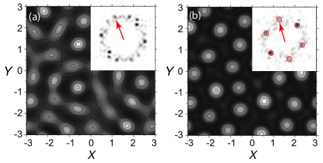
By contrast, the pattern for the larger value of $D_{o}$ clearly shows well developed hexagonal symmetry. These patterns indicate that the formation of hexagonal symmetry is correlated with film depletion near the base of nanopillars. For some parameter sets investigated, there is also evidence of a bifurcation cascade, in which the region halfway in between two adjacent nanopillars generates a parasitic protrusion smaller in amplitude but similar in shape to the primary nanopillars. This cascade behavior resembles the dynamics reported in other thin film instabilities Joo et al. (1991); Krishnamoorthy et al. (1995); Boos and Thess (1999). For this cascade to occur, the value of $D_{o}$ must be sufficiently large such that the growth of the dominant nanopillars consumes a substantial portion of the interstitial fluid mass.

In reviewing images of nanopillar formation in the literature, it is evident that hexagonal symmetry can occur with even small values of $D_{o}$, as shown in Fig. 1(d) for which $D_{o}=1.63$. If the pillars are allowed to grow well beyond the time required for initial contact with the cooler substrate, then the dynamics of growth by thermocapillary stresses will likely continue to draw liquid upwards, thereby thickening the diameter of nanopillars which bridge the gap in between the two substrates. This process will continue to remove film material from the interstitial regions thereby generating conditions favorable to the formation of hexagonal symmetry. In such cases, the hexagonal symmetry is likely established well after the fastest growing peaks make contact with the cooler plate. The mechanism leading to this scenario, however, is not included in the model leading to Eq. (14).

IV.3.2 Effect of substrate tilt

As discussed in Section II.B, the evolution equation for the film height is modified according to Eq. (38) when the confining substrates are subject to a relative tilt. Shown in Fig. (9) are the corresponding results for solutions of $H(X,Y,\tau_{\textrm{top}})$ for the case $h_{o}=100$ nm , $d_{o}=285$ nm and $\Delta T=46\>^{\textrm{o}}\textrm{C}$ subject to increasing inclination angle. The image shown in Fig. (9)(c) corresponds to the inclination angle used in the experiments of Schäffer et al.

Figure 9: Numerical solutions (top view) of the film thickness, $H(X,Y,\tau_{\textrm{top}})$, from Eq. (38) for different inclination angles $\tan(\overline{\varphi})$ of the cooler substrate: (a) $\tan(\overline{\varphi})\!=\!4.8\cdot 10^{-5}$ and $\tau_{\textrm{top}}=1.23$, (b) $\tan(\overline{\varphi})\!=\!4.8\cdot 10^{-4}$ and $\tau_{\textrm{top}}=1.12$, (c) $\tan(\overline{\varphi})\!=\!4.8\cdot 10^{-3}$ and $\tau_{\textrm{top}}=0.86$, (d) $\tan(\overline{\varphi})\!=\!4.8\cdot 10^{-2}$ and $\tau_{\textrm{top}}=0.47$. In all cases, $h_{o}\!=\!100\>$nm, $d_{o}\!=\!285\>$nm and $\Delta T\!=\!46\>^{\textrm{o}}\textrm{C}$. Inclination angle was imposed along the diagonal of the computational domain such that $\tan(\overline{\varphi})/\sqrt{2}=\mid\!\partial D/\partial X\!\mid=\mid\!\partial D/\partial Y\!\mid$. Schematic diagram indicates that upper right corner (lower left corner) is subject to the smallest (largest) wafer separation distance.

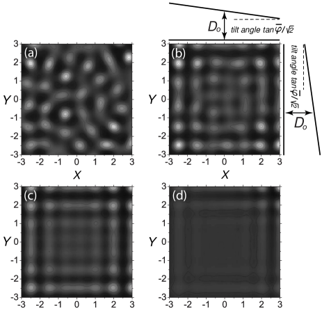
As described in Section II.B, the tilt of the upper substrate was defined by the unit vector $\overrightarrow{T}_{\parallel}=(1,1)/\sqrt{2}$. The top right corner in the images shown corresponds to the region of the film with the smallest gap separation distance; likewise, the bottom left corner represents the region with the largest gap distance. As such, a lateral thermal gradient is established which draws fluid from the bottom left corner into the upper right corner. To conserve mass in the simulations, fluid exiting the top (bottom) boundary was simultaneously replaced by fluid entering the right (left) boundary.

In all the experiments of Schäffer et al. , the confining substrates were subject to a relative tilt $\tan(\varphi)\approx 1\>\mu\textrm{m}/\textrm{cm}$. In rescaled units, $\tan(\overline{\varphi})=\tan(\varphi)/\epsilon$ where $\epsilon=h_{o}/\lambda^{\textrm{TC}}_{\textrm{max}}$. For the experiments in which $h_{o}=100$ nm, $d_{o}=285$ nm and $\Delta T=46\>^{\textrm{o}}\textrm{C}$, $\lambda^{\textrm{TC}}_{\textrm{max}}=4.8~{}\mu\textrm{m}$ [Eq. (27)], such that $\tan(\overline{\varphi})=4.8\cdot 10^{-3}$. The corresponding tilt angle along the $X$ and $Y$ axes for such experiments corresponds to a value of $4.8\cdot 10^{-3}/\sqrt{2}\approx 3.3\cdot 10^{-3}$, which should lead to the formations observed in Fig. (9)(c) if there were no other considerations or artifacts.

As evident from the images (b) - (d), the symmetry of the evolving instability transitions from hexagonal-like to square-like symmetry due to the lateral bias in thermal gradient established by the tilt of the cooler substrate. Even for very small tilt angles, fluid is preferentially transported toward the upper right corner where it accumulates in the form of ridges along the top and right boundaries. This accumulation process establishes secondary and tertiary parallel ridges spaced apart roughly by a distance $\lambda^{\textrm{TC}}_{\textrm{max}}$. At longer times, these ridges are observed to undergo breakup with a similar lateral spacing. A relative tilt of the substrates therefore introduces a strong lateral bias in thermal gradient which triggers pattern formation along the domain boundaries instead of within the interior, where the instability is generally more homogeneously distributed. This specific square symmetry observed is therefore a direct consequence of using inclined substrates within a square computational domain. Modification of the computational domain shape may alter the symmetry observed; however, the nanopillars will still nucleate along cooler regions of the film. Additional studies of the Fourier transforms of the images shown in Fig. (9)(a) - (d) (not shown) confirm that the fastest growing wavelength, $\lambda^{\textrm{TC}}_{\textrm{max}}$, remains unaffected by very small tilt angles. In this respect, the measurements of $\lambda_{\textrm{max}}$ made by Schäffer et al. with a tilted wafer geometry should not have affected comparison to analytic predictions from linear stability theory for films confined by parallel wafers. Given the strong influence of edge behavior on the formation of emerging patterns, however, care should be taken in experiment to ensure that no artifacts, anomalies or asymmetries exist along the edges of a film undergoing nanopillar formation if a particular array symmetry is desirable.

V Conclusion

In this work, we provide evidence that the spontaneous formation of periodic pillar arrays in molten polymer nanofilms confined within closely spaced substrates maintained at different temperatures is due to a thermocapillary instability. If not mass limited, these pillars continue to grow until contact with the cooler substrate is achieved. So long as the initial film thickness and substrate separation distance are sufficiently small that gravitational forces are negligible, there is no critical number for onset of instability. In contrast with the conventional B$\acute{e}$nard-Marangoni instability, nanofilms are prone to formation of elongations no matter how small the transverse thermal gradient. Ultra small gradients, however, lead to large values of the most unstable wavelength. In practice, very large pillar spacings can be difficult to observe or difficult to distinguish from defect mediated bumps which also undergo growth from thermocapillary flow. The linear stability analysis shows that pillar formations are expected in any viscous Newtonian-like nanofilm. Since the shear rates are characteristically small, it is expected that molten materials of many kinds can be modeled as a Newtonian fluid. Pillar arrays formed from polymers like PS or PMMA are of commercial interest, however, since they solidify rapidly in place once the thermal gradient is removed due to their lower glass transition temperatures.

The analytic results obtained, including the energetics of nanopillar formation as described by the Lyapunov functional, confirm that elongations are caused by the predominance of thermocapillary stresses, which far outweigh stabilization by capillary stresses during the later stages of development. The increase in thermocapillary stresses leads to a rapid decrease in the overall free energy of the evolving film. Fourier analysis of the emerging structures also indicates a preference for hexagonal packing although true hexagonal order cannot be achieved if the separation distance is too small since the pillars have insufficient time to grow and self-organize before making contact with the cooler target. Simulations for larger values of $D_{o}=d_{o}/h_{o}$ show well developed and long range hexagonal order. The only limitation of the current analysis is the restriction to films of constant viscosity. While this approximation holds well for simple fluids, it is known that the viscosity of polymer melts like PS and PMMA exhibit a strong dependence on temperature. It is therefore expected that fluid elongations undergo an increase in viscosity as the cooler substrate is approached. We have examined this effect in detail in a separate study Die and concluded that while this cooling effect slows the growth of pillars, it does not affect the pillar spacing in any appreciable way. This is expected since the expression for the most unstable wavelength given by Eq. (27) is independent of the melt viscosity.

The linear stability analysis of an initially flat viscous film of thickness $h_{o}$ subject only to capillary and thermocapillary forces reveals that the normalized gap spacing $d_{o}/h_{o}$ and temperature drop $\Delta T$ strongly affect the value of the most unstable wavelength, $\lambda^{\textrm{TC}}_{\textrm{max}}$, for given material parameters. The analysis indicates that the pillar spacing or array pitch scales as $(\Delta T)^{-1/2}$, which can therefore be tuned in experiment. Direct comparison of $\lambda^{\textrm{TC}}_{\textrm{max}}$ to experimental measurements of Schäffer et al. reveals excellent agreement with the functional dependence on $d_{o}$, namely $\lambda^{\textrm{TC}}_{\textrm{max}}=C_{1}\>{d_{o}}^{1/2}+C_{2}\>{d_{o}}^{-1/2}$. The discrepancies observed are attributed to a number of factors including solvent retention effects in unannealed films and measurements of the array pitch in vitrified films examined after the fluid had experience prolonged contact with the cooler substrate. A number of factors not included in the model can influence the array pitch since the melt is no longer growing in air but migrating and reorganizing along the underside of the cooled wafer.

A linear stability analysis and numerical solutions of the nonlinear evolution equation were also conducted for a tilted cooler substrate. Such a tilt initially establishes both a lateral and vertical thermal gradient. In the experiments of Schäffer et al. , the tilt angle was less than $0.006^{o}$. Numerical simulations of the film height for even very small tilt angles confirm that while the dominant wavelength is unaffected, the in-plane symmetry of evolving elongations can transition from hexagonal to square-like symmetry. This change is caused by thermocapillary influx of fluid into the region subject to a smaller gap width where the effective surface film temperature is cooler due to closer proximity with the cooler tilted substrate. The elongations in this region also grow more rapidly since the effective thermal gradient is larger. These results highlight the importance of boundary conditions in establishing the in-plane symmetry of arrays formed as a result of thermocapillary instability in a tilted geometry. This observation can also be used to advantage to generate large area arrays of different symmetry.

In conclusion, the results presented here strongly suggest that thermocapillary stresses play a crucial if not dominant role in the formation of pillar arrays in molten nanofilms subject to a transverse thermal gradient. According to the linear stability analysis, nanoscale films for which the hydrostatic pressure is completely negligible in comparison to capillary and thermocapillary forces will promote fluid elongations no matter how small the temperature difference between the top (cooler) and bottom (warmer) substrates. Experiments using lower viscosity melts, larger thermal graidents, smaller wafer separation distances, and smaller initial film thicknesses should produce nanostructures with submicron lateral feature sizes. We hope that future studies such as these can assist with the design and fabrication of functional devices by taking advantage of the inherent regularity, smoothness and robustness of self-organized patterns arising from a controllable hydrodynamic instability.

VI Acknowledgement

The authors gratefully acknowledge financial support for this project from the CBET Division of the Engineering Directorate of the National Science Foundation. They also wish to thank the referee for a close reading of this lengthy manuscript.

VII Appendix

To begin, Eq. (19) is re-expressed in terms of the parameter $\chi$ such that

$$\frac{\partial H}{\partial\tau}=-\nabla_{\parallel}\cdot H^{3}\left(\frac{\kappa\overline{Ma}}{2D_{o}\>H(1+\chi H)^{2}}\nabla_{\parallel}H+\frac{1}{3\overline{Ca}}\nabla^{3}_{\parallel}H\right),$$ (A-1)

which is rearranged according to

$$\begin{split}\frac{\partial H}{\partial\tau}=-\!\nabla_{\parallel}\!\cdot\!H^{3}\left[\frac{\kappa\overline{Ma}}{2D_{o}}\left(\frac{1}{H}\!-\!\frac{\chi}{1+\chi H}\!-\!\frac{\chi}{(1+\chi H)^{2}}\right)\nabla_{\parallel}H\right.\\ \left.+\frac{1}{3\overline{Ca}}\nabla^{3}_{\parallel}H\right].\end{split}$$ (A-2)

The term proportional to $\nabla_{\parallel}H$ is further simplified, where

$$\left(\frac{1}{H}\!-\!\frac{\chi}{1+\chi H}\!-\!\frac{\chi}{(1+\chi H)^{2}}\right)\nabla_{\parallel}H=$$

$$\nabla_{\parallel}\left[\ln\left(\frac{H}{1+\chi H}\right)\!+\!\frac{1}{1+\chi H}\right].$$ (A-3)

By introducing the function $\Psi=(\kappa\overline{Ma})/(2D_{o})\{\ln[H/(1+\chi H)]+1/(1+\chi H)\}\!+\!C_{o}$, the evolution equation can be recast as

$$\frac{\partial H}{\partial\tau}=-\nabla_{\parallel}\cdot H^{3}\left[\nabla_{\parallel}\left(\Psi+\frac{1}{3\overline{Ca}}\nabla^{2}_{\parallel}H\right)\right],$$ (A-4)

where $C_{o}$ is a constant of integration. Eq. (A-4) is then multiplied by the quantity $\tilde{\Psi}=\Psi+\nabla^{2}_{\parallel}H/(3\overline{Ca})$ to give

$$\tilde{\Psi}\frac{\partial H}{\partial\tau}=-\tilde{\Psi}\nabla_{\parallel}\cdot H^{3}\nabla_{\parallel}\tilde{\Psi}.$$ (A-5)

Since $\Psi=\Psi(H)$, one can apply Leibnitz’s rule for differentiation to find

$$\frac{\partial I}{\partial\tau}\equiv\frac{\partial}{\partial\tau}\int^{H(\tau)}_{H(\tau=0)}\Psi(S)dS=\Psi\frac{\partial H}{\partial\tau}$$ (A-6)

where $H(\tau=0)=1$ i.e. the initial film is flat and uniform. Evaluation of the function $I$ then gives

$$I\!=\!\frac{\kappa\overline{Ma}}{2D_{o}}\left[H\ln\!\left(\frac{H}{1+\chi H}\!\right)\!+\!\ln(1\!+\!\chi)\right]\!\!+\!C_{1}(H\!-\!1)$$ (A-7)

where $C_{1}$ denotes a second constant of integration.

Equation (A-5) is then integrated over the square domain $A_{\parallel}=\Delta X\Delta Y$:

$$\int_{A_{\parallel}}\left(\frac{\partial I}{\partial\tau}+\frac{1}{3\overline{Ca}}\nabla^{2}_{\parallel}H\frac{\partial H}{\partial\tau}\right)dXdY=$$

$$-\int_{A_{\parallel}}\tilde{\Psi}\nabla_{\parallel}\cdot H^{3}\nabla_{\parallel}\tilde{\Psi}dXdY,$$ (A-8)

where $\tilde{\Psi}\nabla_{\parallel}\cdot(H^{3}\nabla_{\parallel}\tilde{\Psi})$ can be re-expressed as $\nabla_{\parallel}\cdot(\tilde{\Psi}H^{3}\nabla_{\parallel}\tilde{\Psi})-H^{3}(\nabla_{\parallel}\tilde{\Psi})^{2}$. The first term on the right hand side vanishes for a fixed domain subject to periodic boundary conditions; the integral $\int_{A_{\parallel}}(\partial I/\partial\tau)dXdY$ can be rewritten as $d/d\tau\int_{A_{\parallel}}IdXdY$. These simplifications can be used to recast Eq. (VII) into

$$\frac{d}{d\tau}\int_{A_{\parallel}}I(H)dXdY+\frac{1}{3\overline{Ca}}\int_{A_{\parallel}}\nabla^{2}_{\parallel}H\frac{\partial H}{\partial\tau}dXdY=$$

$$\int_{A_{\parallel}}H^{3}\left(\nabla_{\parallel}\tilde{\Psi}\right)^{2}dXdY.$$ (A-9)

A final integration by parts subject to periodic boundary conditions simplifies the second integral on the left hand side such that

$$\int_{A_{\parallel}}\!\nabla^{2}_{\parallel}H\frac{\partial H}{\partial\tau}dXdY\!\! = \!\!\!-\frac{1}{2}\int_{A_{\parallel}}\,\!\!\frac{\partial}{\partial\tau}\left(\nabla_{\parallel}H\right)^{2}dX\!dY$$ (A-10)

$$= \!\!\!-\frac{1}{2}\frac{d}{d\tau}\int_{A_{\parallel}}\!\!\!\left(\nabla_{\parallel}H\right)^{2}dX\!dY$$

Equation (VII) then simplifies to the form

$$\frac{d}{d\tau}\int_{A_{\parallel}}\left[I-\frac{1}{6\overline{Ca}}\left(\nabla_{\parallel}H\right)^{2}\right]dXdY=$$

$$\int_{A_{\parallel}}H^{3}\left(\nabla_{\parallel}\tilde{\Psi}\right)^{2}dXdY.$$ (A-11)

Inserting Eq. (A-7) into Eq. (VII) and noting that volume conservation within the domain $A_{\parallel}$ requires that $\int_{A_{\parallel}}(H-1)dXdY=0$ leads to

$$\begin{split}\frac{d}{d\tau}\int_{A_{\parallel}}\left\{\frac{\kappa\overline{Ma}}{2D_{o}}\left[H\ln\left(\frac{H}{1+\chi H}\right)+\ln(1+\chi)\right]\right.\\ \left.-\frac{1}{6\overline{Ca}}\left(\nabla_{\parallel}H\right)^{2}\right\}dXdY=\\ \int_{A_{\parallel}}H^{3}\left(\nabla_{\parallel}\tilde{\Psi}\right)^{2}dXdY.\end{split}$$ (A-12)

Multiplying Eq. (A-12) by the quantity $-6~{}\overline{Ca}$ produces the final expression for the rate of change of $\mathfrak{F}$, namely

$$\frac{d}{d\tau}\int_{A_{\parallel}}\mathfrak{L}dXdY=-6\overline{Ca}\int_{A_{\parallel}}H^{3}\left(\nabla_{\parallel}\tilde{\Psi}\right)^{2}dXdY\leq 0,$$ (A-13)

where $\mathfrak{L}$ is given by Eq. (34). Since Eq. (A-13) is a non-negative quantity, the thin film seeks configurations of the interface $H$ in time which minimize $\mathfrak{F}$.

References

- Wallraff and Hinsberg (1999) G. M. Wallraff and W. D. Hinsberg, Chem. Rev. 99, 1801 (1999).
- Fuller et al. (2002) S. B. Fuller, E. J. Wilhelm, and J. A. Jacobson, J. Microelectromech. S. 11, 54 (2002).
- Miller et al. (2003) S. M. Miller, S. M. Troian, and S. Wagner, Appl. Phys. Lett. 83, 3207 (2003).
- Gratson et al. (2004) G. M. Gratson, M. J. Xu, and J. A. Lewis, Nature 428, 386 (2004).
- Heckele and Schomburg (2004) M. Heckele and W. K. Schomburg, J. Micromech. Microeng. 14, R1 (2004).
- Chou et al. (1995) S. Y. Chou, P. R. Krauss, and P. J. Renstrom, Appl. Phys. Lett. 67, 3114 (1995).
- Guo (2007) L. J. Guo, Adv. Mat. 19, 495 (2007).
- Menard et al. (2007) E. Menard, M. A. Meitl, Y. Sun, J. Park, D. J. Shir, Y. S. Nam, S. Jeon, and J. A. Rogers, Chem. Rev. 107, 1117 (2007).
- del Campo and Arzt (2008) A. del Campo and E. Arzt, Chem. Rev. 108, 911 (2008).
- Zhang et al. (2003) Z. Zhang, Z. Wang, R. Xing, and Y. Han, Polymer 44, 3737 (2003).
- Petersen and Mayr (2008) J. Petersen and S. G. Mayr, J. Appl. Phys. 103, 023520 (2008).
- Szafraniak et al. (2003) I. Szafraniak, C. Harnagea, R. Scholz, S. Bhattacharyya, D. Hesse, and M. Alexe, Appl. Phys. Lett. 83, 2211 (2003).
- Gonuguntla et al. (2006) M. Gonuguntla, A. Sharma, and S. A. Subramanian, Macromol. 39, 3365 (2006).
- Cuk et al. (2000) T. Cuk, S. M. Troian, C. Hong, and S. Wagner, Appl. Phys. Lett. 77, 2063 (2000).
- Darhuber and Troian (2005) A. A. Darhuber and S. M. Troian, Annu. Rev. Fluid Mech. 37, 425 (2005).
- Darhuber et al. (2003a) A. A. Darhuber, J. P. Valentino, J. M. Davis, S. M. Troian, and S. Wagner, Appl. Phys. Lett. 82, 657 (2003a).
- Darhuber et al. (2003b) A. A. Darhuber, J. M. Davis, S. M. Troian, and W. Reisner, Phys. Fluids 15, 1295 (2003b).
- Darhuber et al. (2003c) A. A. Darhuber, J. P. Valentino, S. M. Troian, and S. Wagner, J. MEMS 12, 873 (2003c).
- Darhuber et al. (2004) A. A. Darhuber, J. Z. Chen, J. M. Davis, and S. M. Troian, Phil. Trans. Royal Soc. London A 17, 1037 (2004).
- Dietzel and Poulikakos (2005) M. Dietzel and D. Poulikakos, Phys. Fluids 17, 102106 (2005).
- Chou and Zhuang (1999) S. Y. Chou and L. Zhuang, J. Vac. Sci. Tech. B 17, 3197 (1999).
- Schäffer et al. (2002) E. Schäffer, S. Harkema, R. Blossey, and U. Steiner, Europhys. Lett. 60, 255 (2002).
- Peng et al. (2004) J. Peng, H. F. Wang, B. Y. Li, and Y. C. Han, Polymer 45, 8013 (2004).
- Chou et al. (1999) S. Y. Chou, L. Zhuang, and L. J. Guo, Appl. Phys. Lett. 75, 1004 (1999).
- Mark (1996) J. Mark, Physical Properties of Polymers Handbook (AIP Press, Woodbury, New York, 1996).
- Schäffer et al. (2003a) E. Schäffer, S. Harkema, M. Roerdink, R. Blossey, and U. Steiner, Macromolecules 36, 1645 (2003a).
- Schäffer (2001) E. Schäffer, Ph.D. thesis, Universitt Konstanz, Konstanz (2001).
- Probstein (1994) R. F. Probstein, Physicochemical Hydrodynamics: An Introduction (2nd Ed.) (J. Wiley & Sons, Inc., New York, 1994).
- Morariu et al. (2004) M. D. Morariu, E. Schäffer, and U. Steiner, Phys. Rev. Lett. 92 (2004).
- Schäffer et al. (2003b) E. Schäffer, S. Harkema, M. Roerdink, R. Blossey, and U. Steiner, Adv. Mater. 15, 514 (2003b).
- Dietzel and Troian (2009) M. Dietzel and S. M. Troian, Phys. Rev. Lett. 104 (2009).
- Morath and Maris (1996) C. J. Morath and H. J. Maris, Phys. Rev. B 54 (1996), 1.
- Scriven and Sternling (1964) L. E. Scriven and C. V. Sternling, J. Fluid Mech. 19, 321 (1964).
- Smith (1966) K. A. Smith, J. Fluid Mech. 24, 401 (1966), part 2.
- Oron et al. (1997) A. Oron, S. H. Davis, and S. G. Bankoff, Rev. Mod. Phys. 69, 931 (1997).
- Vanhook et al. (1995) S. J. Vanhook, M. F. Schatz, W. D. McCormick, J. B. Swift, and H. L. Swinney, Phys. Rev. Lett. 75, 4397 (1995).
- Vanhook et al. (1997) S. J. Vanhook, M. F. Schatz, J. B. Swift, W. D. McCormick, and H. L. Swinney, J. Fluid Mech. 345, 45 (1997).
- (38) The viscosity of polymer melts above the glass transition temperature tends to vary strongly with temperature. As the molten film approaches the cooler substrate, it is expected that its viscosity will exceed the value used in the current analysis. This effect has been investigated in detail Die for the parameter range pertinent to nanofilm experiments. There we find that while this effect slows the growth of pillars somewhat, it barely alters the dominant wavelength . This finding is not surprising - Eq. (27) is independent of the melt viscosity since the fluid flux due to thermocapillary and capillary stresses both scale inversely with the viscosity.
- Leal (2007) L. G. Leal, Fluid Mechanics and Convective Transport Processes (Cambridge University Press, New York, 2007).
- Deen (1998) W. M. Deen, Analysis of Transport Phenomena (Oxford University Press, New York, 1998).
- Bestehorn et al. (2003) M. Bestehorn, A. Pototsky, and U. Thiele, Eur. Phys. J. B 33, 457 (2003).
- Masson and Green (2002) J. L. Masson and P. F. Green, Phys. Rev. E 65 (2002), part 1.
- Lide (1992) D. Lide, CRC Handbook of Chemistry and Physics (CRC Publishing Company, Boca Raton, 1992), 73rd ed.
- Moreira and Demarquette (2001) J. C. Moreira and N. R. Demarquette, J. Appl. Polym. Sci. 82, 1907 (2001).
- VanHook (1996) S. J. VanHook, Ph.D. thesis, University of Texas, Austin, TX (1996).
- Oron (2000) A. Oron, Phys. Fluids 12, 1633 (2000).
- Oron and Rosenau (1994) A. Oron and P. Rosenau, J. Fluid Mech. 273, 361 (1994).
- Cahn and Hilliard (1958) J. W. Cahn and J. E. Hilliard, J. Chem. Phys. 28, 258 (1958).
- García-Turiel and Jérôme (2007) J. García-Turiel and B. Jérôme, Colloid Polym. Sci. 285, 1617 (2007).
- Perlich et al. (2009) J. Perlich, V. Körstgens, M. E., L. Schultz, R. Georgii, and P. Müller-Buschbaum, Macromol. 42, 337 (2009).
- (51) COMSOL Multiphysics®, COMSOL, Inc., Los Angeles, CA 90024.
- Joo et al. (1991) S. W. Joo, S. H. Davis, and S. G. Bankoff, J. Fluid Mech. 230, 117 (1991).
- Krishnamoorthy et al. (1995) S. Krishnamoorthy, B. Ramaswamy, and S. W. Joo, Phys. Fluids 7, 2291 (1995).
- Boos and Thess (1999) W. Boos and A. Thess, Phys. Fluids 11, 1484 (1999).
- (55) M. Dietzel and S. M. Troian, preprint.