Behavioral Simulations in MapReduce

Abstract

In many scientific domains, researchers are turning to large-scale behavioral simulations to better understand important real-world phenomena. While there has been a great deal of work on simulation tools from the high-performance computing community, behavioral simulations remain challenging to program and automatically scale in parallel environments. In this paper we present BRACE (Big Red Agent-based Computation Engine), which extends the MapReduce framework to process these simulations efficiently across a cluster. We can leverage spatial locality to treat behavioral simulations as iterated spatial joins and greatly reduce the communication between nodes. In our experiments we achieve nearly linear scale-up on several realistic simulations.

Though processing behavioral simulations in parallel as iterated spatial joins can be very efficient, it can be much simpler for the domain scientists to program the behavior of a single agent. Furthermore, many simulations include a considerable amount of complex computation and message passing between agents, which makes it important to optimize the performance of a single node and the communication across nodes. To address both of these challenges, BRACE includes a high-level language called BRASIL (the Big Red Agent SImulation Language). BRASIL has object oriented features for programming simulations, but can be compiled to a data-flow representation for automatic parallelization and optimization. We show that by using various optimization techniques, we can achieve both scalability and single-node performance similar to that of a hand-coded simulation.

1 Introduction

Behavioral simulations, also called agent-based simulations, are instrumental in tackling the ecological and infrastructure challenges of our society. These simulations allow scientists to understand large complex systems such as transportation networks, insect swarms, or fish schools by modeling the behavior of millions of individual agents inside the system [6, 11, 13].

For example, transportation simulations are being used to address traffic congestion by evaluating proposed traffic management systems before implementing them [11]. This is a tremendously important problem as traffic congestion cost $87.2 billion and required 2.8 billion gallons of extra fuel and 4.2 billion hours of extra time in the U.S. in 2007 alone [39]. Scientists also use behavioral simulations to model collective animal motion, such as that of locust swarms or fish schools [6, 13]. Understanding these phenomena is crucial, as they directly affect human food security [23].

Despite their huge importance, it remains difficult to develop large-scale behavioral simulations. Current systems either offer high-level programming abstractions, but are not scalable [21, 30, 33], or achieve scalability by hand-coding particular simulation models using low-level parallel frameworks, such as MPI [44].

This paper proposes to close this gap by bringing database-style programmability and scalability to agent-based simulations. Our core insight is that behavioral simulations may be regarded as computations driven by large iterated spatial joins. We introduce a new simulation engine, called BRACE (Big Red Agent-based Computation Engine), that extends the popular MapReduce dataflow programming model to these iterated computations. BRACE embodies a high-level programming language called BRASIL, which is compiled into an optimized shared-nothing, in-memory MapReduce runtime. The design of BRACE is motivated by the requirements of behavioral simulations, explained below.

1.1 Requirements for Simulation Platforms

We have identified several key features that are necessary for a generic behavioral simulation platform.

(1) Support for Complex Agent Interaction. Behavioral simulations include frequent local interactions between agents. In particular, agents may affect the behavior decisions of other agents, and multiple agents may issue concurrent writes to the same agent. A simulation framework should support a high degree of agent interaction without excessive synchronization or rollbacks. This precludes discrete event simulation engines or other approaches based on task parallelism and asynchronous message exchange.

(2) Automatic Scalability. Scientists need to scale their simulations to millions or billions of agents to accurately model phenomena such as city-wide traffic or swarms of insects [6, 13, 20]. These scales make it essential to use data parallelism to distribute agents across many nodes. This is complicated by the interaction between agents, which may require communication between several nodes. Rather than requiring scientists to write complex and error-prone parallel code, the platform should automatically distribute agents to achieve scalability.

(3) High Performance. Behavioral simulations are often extremely complex, involving sophisticated numerical computations and elaborate decision procedures. Much existing work on behavioral simulations is from the high-performance computing community, and they frequently resort to hand-coding specific simulations in a low-level language to achieve acceptable performance [20, 34]. A general purpose framework must be competitive with these hand-coded applications in order to gain acceptance.

(4) Commodity Hardware. Historically, many scientists have used large shared-memory supercomputer systems for their simulations. Such machines are tremendously expensive, and cannot scale beyond their original capacity. We believe that the next generation of simulation platforms will target shared-nothing systems and will be deployed on local clusters or in the cloud on services like Amazon’s EC2 [2].

(5) Simple Programming Model. Domain scientists have shown their willingness to try simulation platforms that provide simple, high-level programming abstractions, even at some cost in performance and scalability [21, 30, 33]. Nevertheless, a behavioral simulation framework should provide an expressive and high-level programming model without sacrificing performance.

1.2 Contributions

We begin our presentation in Section 2.1 by describing important properties of behavioral simulations that we leverage in our platform. We then move on to the main contributions of this paper:

• We show how MapReduce can be used to scale behavioral simulations across clusters. We abstract these simulations as iterated spatial joins and introduce a new main memory MapReduce runtime that incorporates optimizations motivated by the spatial properties of simulations (Section 3).

• We present a new scripting language for simulations that compiles into our MapReduce framework and allows for algebraic optimizations in mappers and reducers. This language hides all the complexities of modeling computations in MapReduce and parallel programming from domain scientists (Section 4).

• We perform an experimental evaluation with two real-world behavioral simulations that shows our system has nearly linear scale-up and single-node performance that is comparable to a hand-coded simulation. (Section 5).

We review related work in Section 6 and conclude in Section 7.

2 Background

In this section, we introduce some important properties of behavioral simulations and review the MapReduce programing model. In the next section we exploit these properties to abstract the computations in the behavioral simulations and use MapReduce to efficiently process them.

2.1 Properties of Behavioral Simulations

Behavioral simulations model large numbers of individual agents that interact in a complex environment. Unlike scientific simulations that can be modeled as systems of equations, agents in a behavioral simulation can execute complex programs that include non-trivial control flow. Nevertheless, most behavioral simulations have a similar structure, which we introduce below. We will use a traffic simulation [48] and a fish school simulation [13] as running examples. Details on these simulation models can be found in Appendix C.

The State-Effect Pattern. Most behavioral simulations use a time-stepped model in which time is discretized into “ticks” that represent the smallest time period of interest. Events that occur during the same tick are treated as simultaneous and can be reordered or parallelized. This means that an agent’s decisions cannot be based on previous actions made during the same tick. An agent can only read the state of the world as of the previous tick. For example, in the traffic simulation, each car inspects the positions and velocities of other cars as of the beginning of the tick in order to make lane changing decisions.

In previous work on scaling computer games, we proposed a model for this kind of time-stepped behavior called the state-effect pattern [45, 46]. The basic idea is to separate read and write operations in order to limit the synchronization necessary between agents. In the state-effect pattern, the attributes of an agent are separated into states and effects, where states are public attributes that are updated only at tick boundaries, and effects are used for intermediate computations as agents interact. Since state attributes remain fixed during a tick, they only need to be synchronized at the end of each tick. Furthermore, each effect attribute has an associated decomposable and order-independent combinator function for combining multiple assignments during a tick. This allows us to compute effects in parallel and combine the results without worrying about concurrent writes. For example, the fish school simulation uses vector addition so that each fish may combine the orientation of nearby fish into an effect attribute. Since vector addition is commutative, we can process these assignments in any order.

In the state-effect pattern, each tick is divided into two phases: the query phase and the update phase, as shown in the figure on the right. In the query phase, each agent queries the state of the world and assigns effect values, which are combined using the appropriate combinator function. To ensure the property that the actions during a tick are conceptually simultaneous, state variables are read-only during the query phase and effect variables are write-only.

In the update phase, each agent can read its state attributes and the effect attributes computed from the query phase; it uses these values to compute the new state attributes for the next tick. In the fish school simulation, the orientation effects computed during the query phase are read during the update phase to compute a fish’s new velocity vector, represented as a state attribute. In order to ensure that updates do not conflict, each agent can only read and write its own attributes during the update phase. Hence, the only way that agents can communicate is through effect assignments in the query phase. We classify effect assignments into local and non-local assignments. In a local assignment, an agent updates one of its own effect attributes; in a non-local assignment, an agent writes to an effect attribute of a different agent.

The Neighborhood Property. The state-effect pattern can be used to limit the synchronization necessary during a tick, but it is still possible that every agent needs to query every other agent in the simulated world to compute its effects. We observe that this rarely occurs in practice. In particular, we observe that most behavioral simulations are eminently spatial, and simulated agents can only interact with other agents that are close according to a distance metric [28]. For example, a fish can only observe other fish within a limited distance $\rho$.

2.2 MapReduce

Since its introduction in 2004, MapReduce has become one of the most successful models for processing long running computations in distributed shared-nothing environments[16]. While it was originally designed for very large batch computations, MapReduce is ideal for behavioral simulations because it provides automatic scalability, which is one of the key requirements for next-generation platforms. By varying the degree of data partitioning and the corresponding number of map and reduce tasks, the same MapReduce program can be run on one machine or one thousand.

The MapReduce programming model is based on two functional programming primitives that operate on key-value pairs. The map function takes a key-value pair and produces a set of intermediate key-value pairs, $\textsf{map}:(k_{1},v_{1})\to[(k_{2},v_{2})]$, while the reduce function collects all of the intermediate pairs with the same key and produces a value, $\textsf{reduce}:(k_{2},[v_{2}])\to[v_{3}]$. Since simulations consist of many ticks, we will use an iterative MapReduce model in which the output of the reduce step is fed into the next map step. Formally, this means that we change the output of the reduce step to be $[(k3,v3)]$.

3 MapReduce for Simulations

In this section, we abstract behavioral simulations as computations driven by iterated spatial joins and show how they can be expressed in the MapReduce framework (Section 3.1). We then propose a system called BRACE to process these joins efficiently (Section 3.3).

3.1 Simulations as Iterated Spatial Joins

effects	$\mathbf{map_{1}^{t}}$	$\mathbf{reduce_{1}^{t}}$	$\mathbf{map_{2}^{t}}$	$\mathbf{reduce_{2}^{t}}$	$\mathbf{map_{1}^{t+1}}$
local	updatet-1	queryt	—	—	updatet
	distributet				distributet+1
non-	updatet-1	local	—	global	updatet
local	distributet	effectt		effectt	distributet+1

Table 1: The state-effect pattern in MapReduce.

In Section 2.1, we observed that behavioral simulations have two important properties: the state-effect pattern and the neighborhood property. The state-effect pattern essentially characterizes behavioral simulations as iterated computations with two phases: a query phase in which agents inspect their environment to compute effects, and an update phase in which agents update their own state.

The neighborhood property introduces two important restrictions on each of these phases, visibility and reachability. We say that the visible region of an agent $a$ is the region of space containing agents that $a$ can read from or assign effects to. Agent $a$ needs access to all the agents in its visible region to compute its query phase. Thus a simulation in which agents have small visible regions requires less communication than one with very large or unbounded visible regions. Similarly, we can define an agent’s reachable region as the region that the agent can move to after the update phase. This is essentially a measure of how much the spatial distribution of agents can change between ticks. When agents have small reachable regions, a spatial partitioning of the agents is likely to remain balanced for several ticks. Frequently an agent’s reachable region will be a subset of its visible region (an agent can’t move farther than it can see), but this is not required.

We observe that since agents only query other agents within their visible regions, processing a tick is similar to a spatial self-join from the database literature [31]. We join each agent with the set of agents in its visible region and perform the query phase using only these agents. During the update phase, agents move to new positions within their reachable regions and we perform a new iteration of the join during the next tick. We will use these observations to parallelize behavioral simulations efficiently in the MapReduce framework.

3.2 Iterated Spatial Joins in MapReduce

In this section, we show how to model spatial joins in MapReduce. A formal version of this model is included in Appendix A. MapReduce has often been criticized for being inefficient at processing joins [47] and also inadequate for iterative computations without modification [18]. However, the spatial properties of simulations will allow us to process them effectively without excessive communication. Our basic strategy is to use a technique presented by Zhang et al. to compute a spatial join in MapReduce [50]. Each map task is responsible for spatially partitioning agents into a number of disjoint regions, and the reduce tasks join the agents using their visible regions.

The map tasks use a spatial partitioning function to assign each agent to a disjoint region of space. This function might divide the space into a regular grid or might perform some more sophisticated spatial decomposition. Each reducer will process one such partition. The set of agents assigned to a particular partition is called that partition’s owned set. Note that we cannot process each partition completely independently because each agent needs access to its visible region, and this region may intersect several partitions. To address this, we can define the visible region of a partition as the region of space visible to some point in the partition. The map task will then replicate each agent $a$ to every partition that contains $a$ in its visible region.

Table 1 shows how the phases of the state-effect pattern are assigned to map and reduce tasks. For simulations with only local effect assignments, a tick $t$ begins when the first map task, $\mathsf{map}_{1}^{t}$, assigns each agent to a partition (distribute^t). Each reducer is assigned a partition and receives every agent that falls within its owned set as well as replicas of every agent that falls within its visible region. These are exactly the agents necessary to process the query phase of the owned set (query^t). The reducer, $\mathsf{reduce}_{1}^{t}$, outputs a copy of each agent it owns after executing the query phase and updating the agent’s effects. The tick ends when the next map task, $\mathsf{map}_{1}^{t+1}$, executes the update phase (update^t).

While this two-step approach works well for simulations that have only local effects, it does not handle non-local effect assignments. Recall that a non-local effect is an effect assignment by some agent $a$ to some other agent $b$ within $a$’s visible region. For example, if we were to extend the fish simulation to include predators, then we would model a shark attack as a non-local effect assignment from the shark to the fish. Non-local effects require communication during the query phase. We implement this communication using two MapReduce passes, as illustrated in Table 1. The first map task, $\mathsf{map}_{1}^{t}$, is the same as before. The first reduce task, $\mathsf{reduce}_{1}^{t}$, performs only effect assignments to its local replicas (local effect^t). These partially aggregated effect values are then distributed to the partitions that own them, where they are combined by the second reduce task, $\mathsf{reduce}_{2}^{t}$. This computes the final value for each aggregate (global effect^t). As before, the update phase is processed in the next map task, $\mathsf{map}_{1}^{t+1}$. Note that the second map task, $\mathsf{map}_{2}^{t}$, is only necessary for distribution, but does not perform any computation and can be eliminated in an implementation. We call this model map-reduce-reduce.

Our map-reduce-reduce model relies heavily on the neighborhood property. The number of replicas that each map task must create depends on the size of the agent’s visible regions, and the frequency with the agents change partitions depends on the size of their reachable regions.

3.3 The BRACE MapReduce Runtime

In this section we describe a MapReduce implementation that takes advantage of the state-effect pattern and the neighborhood property. We introduce BRACE, the Big Red Agent Computation Engine, our platform for scalable behavioral simulations. BRACE includes a MapReduce runtime especially optimized for the iterated spatial joins discussed in Section 3.1. We have developed a new system rather than using an existing MapReduce implementation such as Hadoop [24] because behavioral simulations have considerably different characteristics than traditional MapReduce applications such as search log analysis. The goal of BRACE is to process a very large number of ticks efficiently, and to avoid I/O or communication overhead while providing features such as fault tolerance. We describe the main features of our runtime below.

Shared-Nothing, Main-Memory Architecture. In behavioral simulations, we expect data volumes to be modest, so BRACE executes map and reduce tasks entirely in main memory. For example, a simulation with one million agents whose state and effect fields occupy 1 KB on average requires roughly 1 GB of main memory. Even larger simulations with orders of magnitude more agents will still fit in the aggregate main memory of a cluster. Since the query phase is computationally expensive, partition sizes are limited by CPU cycles rather than main memory size.

Figure 1: BRACE Architecture Overview

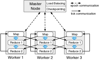
Figure 1 shows the architecture of BRACE. As in typical MapReduce implementations, a master node is responsible for cluster coordination. Unlike in traditional MapReduce runtimes, BRACE’s master node only interacts with worker nodes every epoch, which corresponds to a fixed number of ticks. The intuition is that iterations will be quickly processed in main memory by the workers, so we wish to amortize the overheads related to fault tolerance and load balancing. In addition, we carefully allocate tasks of map-reduce-reduce iterations to workers, so that we diminish communication overheads within and across iterations.

Fault Tolerance. Traditional MapReduce runtimes provide fault tolerance by storing output to a replicated file system and automatically restarting failed tasks. Since we expect ticks to be quite short and they are processed in main memory, it would be prohibitively expensive to write output to stable storage between every tick. Furthermore, since individual ticks are short, the benefit from restarting a task is likely to be small.

We employ epoch synchronization with the master to trigger coordinated checkpoints [19] of the main memory of the workers. As the master determines a pre-defined tick boundary for checkpointing, the workers can write their checkpoints independently without global synchronization. As we expect iterations to be short, failures are handled by re-execution of all iterations since the last checkpoint, a common technique in scientific simulations. In fact, we can leverage previous literature to tune the checkpointing interval to minimize the total expected runtime of the whole computation [14].

Partitioning and Load Balancing. As we have observed in Section 3.2, bounded reachability implies that a given spatial partitioning will remain effective for a number of map-reduce-reduce iterations. Our runtime uses that observation to keep data partitioning stable over time and re-evaluates it at epoch boundaries.

At the beginning of the simulation, the master computes a partitioning function based on the visible regions of the agents and then broadcasts this partitioning to the worker nodes. Each worker becomes responsible for one region of the partitioning. While agents change partitions slowly, over time the overall spatial distribution may change quite dramatically. For example, the distribution of traffic on a road network is likely to be very different at morning rush hour than at evening rush hour. This would cause certain nodes to become overloaded if we used the same partitioning in both cases. To address this, the master periodically requests statistics from the workers about the number of agents in the owned region and the communication and processing costs. The master then decides on repartitioning by balancing the cost of redistribution with its expected benefit. If the master decides to modify the partitioning, it broadcasts the new partitioning to all workers. The workers then switch to the new partitioning at a specified epoch boundary.

Collocation of Tasks. Since simulations run for many iterations, it is important to avoid unnecessary communication between map and reduce tasks. We accomplish this by collocating the map and reduce tasks for a tick on the same node so that agents that do not switch partitions can be sent between tasks via fast memory rather than the network. Since agents have limited reachable regions, the owned set of each partition is likely to remain relatively stable across ticks, and so will remain on the same node. Agents still need to be replicated, but their original copies do not have to be redistributed. This idea was previously explored by the Phoenix project for SMP systems [49] and the Map-Reduce-Merge project for individual joins [47], but it is particularly important for long-running behavioral simulations.

Figure 1 shows how collocation works when we allow non-local effect assignments. Solid arrows indicate the flow of agents during a tick. Each node processes a map task and two reduce tasks as described in Section 3.1. The map task replicates agents as appropriate and sends all of the agents that remain in the same partition to the reduce task on the same node. The first reducer computes local effects and sends any updated replicas to the second reduce phase at other nodes. The final reducer computes the final effects and sends them to the map task on the same node. Because of the neighborhood property, many agents will be processed on the same node during the next tick.

4 Programming Agent Behavior

In this section, we show how to offer a simple programming model for a domain scientist, targeting the last requirement of Section 1.1. MapReduce is set-based; a program describes how to process all of the elements in a collection. Simulation developers prefer to describe the behavior of their agents individually, and use message-passing techniques to communicate between agents. This type of programming is closer to the scientific models that describe agent behavior.

We introduce a new programming language – BRASIL, the Big Red Agent SImulation Language. BRASIL embodies agent centric programming with explicit support for the state-effect pattern, and performs further algebraic optimizations. It bridges the mental model of simulation developers and our MapReduce processing techniques for behavioral simulations. We provide an overview of the main features of BRASIL (Section 4.1) and describe algebraic optimization techniques that can be applied to our scripts (Section 4.2). Formal semantics for our language as well as the proofs of theorems in this section are provided in Appendix B.1.

4.1 Overview of BRASIL

BRASIL is an object-oriented language in which each object corresponds to an agent in the simulation. Agents in BRASIL are defined in a class file that looks superficially similar to Java. The programmer can specify fields, methods, and constructors, and these can each either be public or private. Unlike in Java, however, each field in a BRASIL class must be tagged as either state or effect. The BRASIL compiler then enforces the read-write restrictions of the state-effect pattern over those fields as described in Section 2.1. Figure 2 illustrates an example of a simple two-dimensional fish simulation; in this simulation, the fish swim about randomly, but avoid each other through the use of imaginary repulsion “forces”.

class Fish {
  // The fish location
  public state float x : (x+vx); #range[-1,1];
  public state float y : (y+vy); #range[-1,1];

  // The latest fish velocity
  public state float vx : vx + rand() + avoidx / count * vx;
  public state float vy : vy + rand() + avoidy / count * vy;

  // Used to update our velocity
  private effect float avoidx : sum;
  private effect float avoidy : sum;
  private effect int count : sum;

  /** The query-phase for this fish. */
  public void run() {
    // Use "forces" to repel fish too close
    foreach(Fish p : Extent<Fish>) {
       p.avoidx <- 1 / abs(x - p.x);
       p.avoidy <- 1 / abs(y - p.y);
       p.count  <- 1;
    }}}

Figure 2: Class for Simple Fish Behavior

Recall that the state-effect pattern divides the computation into a query and an update phase. In BRASIL, the query phase for an agent class is expressed by its run() method. State fields remain read-only and all effect assignments are aggregated using the aggregate function specified at the effect field declaration. Effect fields are similar to aggregator variables in Sawzall [37]; indeed, we use the Sawzall operator <- for writing to effect fields. In our fish simulation, for example, each fish repels nearby fish via a “force” inversely proportional to the distance between them. The update phase is specified as a collection of update rules attached to each state field. These rules can only read values of other fields in this agent. In our example, fish velocity vectors get updated based on the avoidance factors and then perturbed by a random amount.

There are some important restrictions in BRASIL’s programming constructs. First, BRASIL only supports iteration over a set or list via a foreach-loop. This eliminates arbitrary looping, which is not available in algebraic database languages. Second, there is an interplay between foreach-loops and effects: effect variables can only be read outside of a foreach-loop, and all assignments within a foreach-loop are aggregated. This powerful restriction allows us to treat the entire program, and not just the communication across map and reduce operations, as a data-flow query plan.

BRASIL also has a special programming construct to enforce the neighborhood property outlined in Section 2.1. Every state field that encodes spatial location may be tagged with a visibility and reachability constraint. While it is possible to generalize this concept to arbitrary constraints, in our current implementation the constraints are (hyper)rectangles. For example, the constraint attached to the x field in Figure 2 means that $[-1,1]$ is the interval that this fish can inspect or move with respect to the x coordinate. In our fish example, the foreach-loop will therefore only be able to affect fish within this range. In addition, the update rule is guaranteed to crop any changes to the x coordinate to at most one unit.

Note that visibility has an interplay with agent references: it is possible that a reference to another agent is fine initially, but violates the visibility constraint as that other agent moves relative to the one holding the reference. For that reason, BRASIL employs weak reference semantics for agent references, similar to weak references in Java. If another agent moves outside of the visible region, then all references to it will resolve to nil.

Note that this gives a different semantics for visibility than the one present in Section 3. BRASIL uses visibility to determine how agent references are resolved, while the BRACE runtime uses visibility to determine agent replication and communication. The BRASIL semantics are preferable for a developer, because they are easy to understand and hide MapReduce details. Fortunately, as we prove formally in Appendix B.1, these are equivalent.

Theorem 11 missing missing missing

The BRASIL semantics for visibility and the BRACE implementation of visibility are equivalent.

While programming features in BRASIL may seem unusual, everything in the language follows from the state-effect pattern and neighborhood property. As these are natural properties of behavioral simulations, programming these simulations becomes relatively straightforward. Indeed, a large part of our traffic simulation in Section 5.1 was implemented by a domain scientist.

4.2 Optimization

We compile BRASIL into a well-understood data-flow language. In our previous work on computer games, we used the relational algebra to represent our data flow [45]. However, for distributed simulations, we have found the monad algebra [7, 29, 36, 42] – the theoretical foundation for XQuery [29] – to be a much more appropriate fit. In particular, the monad algebra has a map primitive for descending into the components of its nested data model; this makes it a much more natural companion to MapReduce than the relational algebra.

We present the formal translation to the monad algebra in Appendix B, together with several theorems regarding its usage in optimization. Most of these optimizations are the same as those that would be present in a relational algebra query plan: algebraic rewrites and automatic indexing. In fact, any monad algebra expression on flat tables can be converted to an equivalent relational algebra expression and vice versa [36]; rewrites and indexing on the relational form carry back into the monad algebra form. In particular, many of the techniques used by Pathfinder [43] to process XQuery with relational query plans apply to the monad algebra.

Effect Inversion. An important optimization that is unique to our framework involves the assignment of non-local effects. If non-local effect assignments can be eliminated, then we are able to process our MapReduce computations with one MapReduce pass instead of two (Section 3). Consider again the program of Figure 2. We may rewrite its foreach-loop as

  foreach(Fish p : Extent<Fish>) {
       avoidx <- 1 / abs(p.x - x);
       avoidy <- 1 / abs(p.y - y);
       count <- 1;
  }

This rewritten expression does not change the results of the simulation, but only assigns effects locally.

There are two main results regarding effect inversion. While we prove them formally in Appendix B.2, we can state them informally here, and give some intuition regarding their usage.

Theorem 22 missing missing missing

Effect inversion is always possible if there are no visibility constraints.

When there are no visibility constraints, each agent can read any other agent. Hence, we can produce a script where an agent simulates the behavior of other agents, checks for effects that are assigned to itself, and then assign them locally. Unfortunately, this new script is clearly much more computationally expensive. Hence, to be useful in practice, we need to use other optimization techniques to simplify the new script.

Effect inversion is not always possible when the simulation has visibility constraints. Intuitively, an agent may use non-local effects to act as a communication proxy between two other agents that are not visible to one another. However, the state-effect pattern ensures that an agent can only receive information from another agent if they have a third (not necessarily distinct) agent that is visible to both. This provides us with another result.

Theorem 33 missing missing missing

If the visibility constraint on a script is a distance bound, there is an equivalent script with a constraint at most twice that distance bound that has only local effect assignments.

Increasing the visibility bound increases the number of replicas that have to store at each node. Hence this optimization eliminates the extra communication round at the cost of more information to be sent during the remaining communication round.

5 Experiments

In this section, we present experimental results using two distinct real-world behavioral simulation models we have coded using BRACE. We focus on the following: (i) We validate the effectiveness of the BRASIL optimizations introduced in Section 4.2. In fact, these optimizations allow us to approach the efficiency of hand-optimized simulation code (Section 5.2); (ii) We evaluate BRACE’s MapReduce runtime implementation over a cluster of machines. We measure simulation scale-up via spatial data partitioning as well as load balancing (Section 5.3).

5.1 Setup

Implementation. The prototype BRACE MapReduce runtime is implemented in C++ and uses MPI for inter-node communication. Our BRASIL compiler is written in Java and directly generates C++ code that can be compiled with the runtime.

Our prototype includes a generic KD-tree based spatial index capability [4]. We use a simple rectilinear grid partitioning scheme, which assigns each grid cell to a separate slave node, A one-dimensional load balancer periodically receives statistics from the slave nodes, including computational load and number of owned agents; from these it heuristically computes a new partition trying to balance improved performance against estimated migration cost. Checkpointing is not yet integrated into BRACE’s implementation. We believe this is not a problem for the cluster sizes we evaluate, given the low likelihood of worker failure during a computation.

We plan to integrate more sophisticated algorithms for all these components in future work. But our current prototype already demonstrates good performance and automatic scaling of realistic behavioral simulations written in BRASIL.

Simulation Workloads. We have implemented realistic traffic and fish school simulations in BRASIL. The traffic simulation includes the lane-changing and acceleration models of the state-of-the-art, open-source MITSIM traffic simulator [48]. MITSIM is a single-node program, so we compare its performance against our BRASIL reimplementation of its model also running on a single node. We simulate a linear segment of highway, and scale-up the size of the problem by extending the length of the segment.

The fish simulation implements a recent model of information flow in animal groups [13]. In this model the “ocean” is unbounded, and the spatial distribution of fish changes dramatically as “informed individuals” guide the movements of others in the school.

Neither of these simulations uses non-local effect assignments; therefore we need only a single reducer per node. To evaluate our effect inversion optimization, we modified the fish simulation to create a predator simulation that uses non-local assignments. It is similar in spirit to artificial society simulations [28]. Appendix C describes these simulation models in more detail. We measure total simulation time in our single-node experiments and tick throughput (agent ticks per second) when scaling up over multiple nodes. In all measurements we eliminate start-up transients by discarding initial ticks until a stable tick rate is achieved.

Hardware Setup. We ran all of our experiments in the Cornell Web Lab cluster [3]. The cluster contains 60 nodes interconnected by a pair of 1 gigabit/sec Port Summit X450a Ethernet Switches. Each node has two Quad Core Intel Xeon, 2.66GHz, processors with 4MB cache each and 16 GB of main memory.

5.2 BRASIL Optimizations

Figure 3: Traffic: Indexing vs. Seg. Length

Figure 4: Fish: Indexing vs. Visibility

Figure 5: Predator: Effect Inversion

Figure 6: Traffic: Scalability

Figure 7: Fish: Scalability

Figure 8: Fish: Load Balancing

We first compare the single-node performance of our traffic simulation to MITSIM. The main optimization in this case is spatial indexing. For a meaningful comparison, we validate the aggregate traffic statistics produced by our BRASIL reimplementation against those produced by MITSIM. Details of our validation procedure appear in Appendix C.

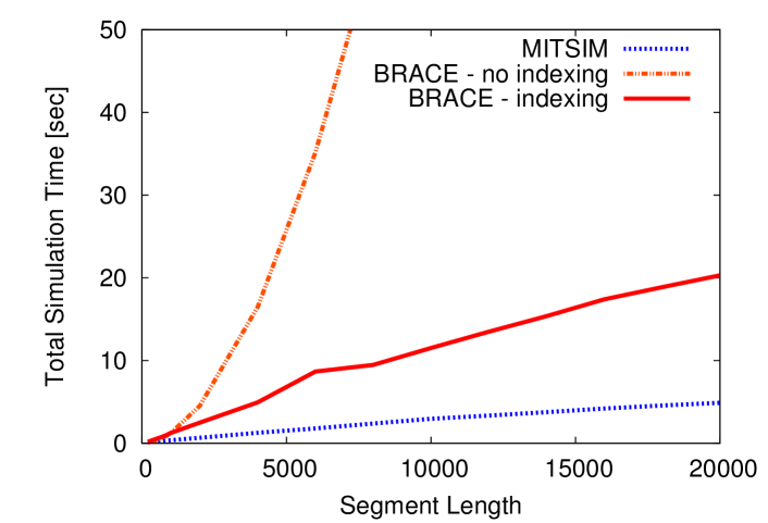
Figure 5 compares the performance of MITSIM against our BRACE reimplementation of its model. Without spatial indexing, BRACE’s performance degrades quadratically with increasing segment length. This is expected: In this simulation, the number of agents grows linearly with segment length; and without indexing every vehicle enumerates and tests every other vehicle during each tick. With spatial indexing enabled, BRACE converts this behavior to an orthogonal range query, resulting in log-linear growth, as confirmed by Figure 5. BRACE’s spatial indexing achieves performance that is comparable, but inferior to MITSIM’s hand-coded nearest-neighbor implementation. Our optimization techniques generalize to nearest-neighbor indexing, and adding this to BRACE is planned future work. With this enhancement, we expect to achieve performance parity with MITSIM.

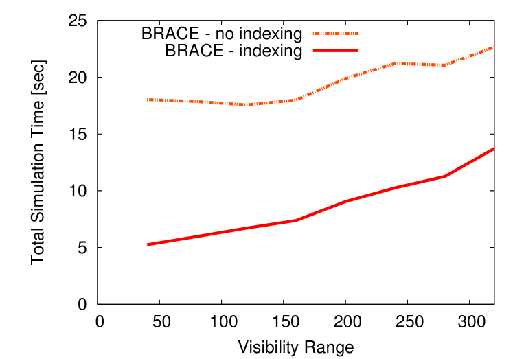
We observed similar log-linear versus quadratic performance when scaling up the number of agents in the fish simulation in a single node. We thus omit these results. When we increase the visibility range, however, the performance of the KD-tree indexing decreases, since more results are produced for each index probe (Figure 5). Still, indexing yields from two to three times improvement over a range of visibility values.

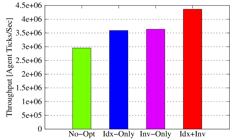
In addition to indexing, we also measure the performance gain of eliminating non-local effect assignments through effect inversion. Only the predator simulation has non-local effect assignments, so we report results exclusively on this model. We run two versions of the predator simulation, one with non-local assignments and the other with non-local assignments eliminaed by effect inversion. We run both scripts with and without KD-tree indexing enabled on 16 slave nodes, and with BRACE configured to have two reduce passes in the first case and only a single reduce pass in the second case. Our results are displayed in Figure 5. Effect inversion increases agent tick throughput from 3.59 million (Idx-Only) to 4.36 million (Idx+Inv) with KD-tree indexing enabled, and from 2.95 million (No-Opt) to 3.63 million (Inv-Only) with KD-tree indexing disabled. This represents an improvement of more than 20% in each case, demonstrating the importance of this optimization.

5.3 Scalability of the BRACE Runtime

We now explore the parallel performance of BRACE’s MapReduce runtime on the traffic and fish school simulations as we scale the number of slave nodes from 1 to 36. The size of both simulations is scaled linearly with the number of slaves, so we measure scale-up rather than speed-up.

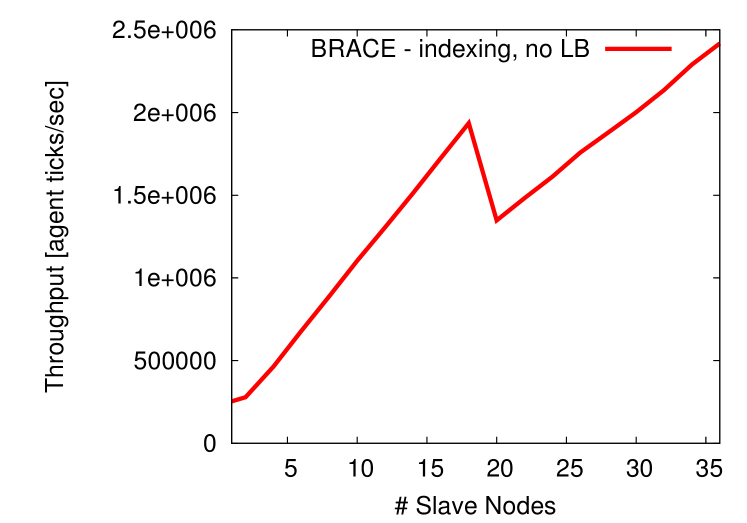
The traffic simulation represents a linear road segment with constant up-stream traffic. As a result, the distribution on the segment is nearly uniform, and load is always balanced among the nodes. Therefore, throughput grows linearly with the number of nodes even if load balancing is disabled (Figure 8). The sudden drop around 20 nodes is an artifact of the multi-switch architecture of the Web Lab cluster on which we ran our experiments: Performance degrades when not all nodes can be chosen on the same switch.

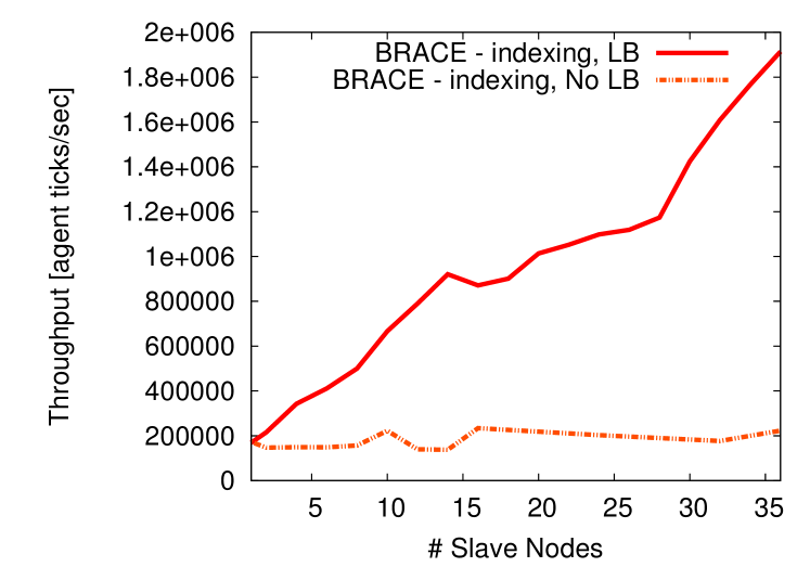
In the fish simulation, fish move in schools led by informed individuals [13]. In our experiment, there are two classes of informed individuals, trying to move in two different fixed directions. The spatial distribution of fish, and consequently the load on each slave node, changes over time. Figure 8 shows the scalability of this simulation with and without load balancing. Without load balancing, two fish schools eventually form in nodes at the extremes of simulated space, while the load at all other nodes falls to zero. With load balancing, partition grids are adjusted periodically to assign roughly the same number of fish to each node, so throughput increases linearly with the number of nodes.

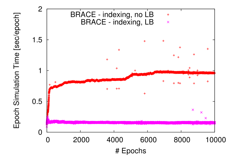
Figure 8 confirms this. With load balancing enabled, the time per simulation epoch is essentially flat; with load balancing disabled, the epoch time gradually increases to a value that reflects all agents being simulated by only two nodes.

6 Related Work

Much of the existing work on behavioral simulations has focused on task-parallel discrete event simulation systems [9, 35, 15, 32, 51]. Such systems employ either conservative or optimistic protocols to detect conflicts and preempt or rollback simulation tasks. The strength of local interactions and the time-stepped model used in behavioral simulations lead to unsatisfactory performance, as shown in attempts to adapt discrete event simulators to agent-based simulations [27, 26].

Platforms specifically targeted at agent-based models have been developed, such as Swarm [33], Mason [30], and Player/Stage [21]. These platforms offer tools to facilitate simulation programming, but most rely on message-passing abstractions with implementations inspired by discrete event simulators, so they suffer in terms of performance and scalability. A few recent systems attempt to distribute agent-based simulations over multiple nodes without exploiting applications properties such as visibility and time-stepping [25, 38]. This leads either to poor scale-up or to unrealistic restrictions on agent interactions.

Regarding join processing with MapReduce, Zhang et al. [50] compute spatial joins by an approach similar to ours when only local effect assignments are allowed. Their mapper partitions are derived using spatial index techniques rather than by reasoning about the application program, and they do not discuss iterated joins, an important consideration for our work. Locality optimizations have been studied for MapReduce on SMPs [49] and for MapReduceMerge [47]; in this paper we consider the problem in a distributed main memory MapReduce runtime.

Data-driven parallelization techniques have also been studied in parallel databases [17, 22] and data parallel programming languages [5, 40]. However, it is unnatural and inefficient to use either SQL or set-operations exclusively to express flexible computation over individuals as required for behavioral simulations.

Given this situation, behavioral simulation developers have resorted to hand-coding parallel implementations of specific simulation models [20, 34], or trading model accuracy for scalability and ease of implementation [8, 44]. To the best of our knowledge, our approach is the first to bring both programmability and scalability through data parallelism to behavioral simulations.

7 Conclusions

In this paper we show how MapReduce can be used to scale behavioral simulations across clusters by abstracting these simulations as iterated spatial joins. To efficiently distribute these joins we leverage several properties of behavioral simulations to get a shared-nothing, in-memory MapReduce framework called BRACE, which exploits collocation of mappers and reducers to bound communication overhead. In addition, we present a new scripting language for our framework called BRASIL, which hides all the complexities of modeling computations in MapReduce and parallel programming from domain scientists. BRASIL scripts can be compiled into our MapReduce framework and allow for algebraic optimizations in mappers and reducers. We perform an experimental evaluation with two real-world behavioral simulations to show that BRACE has nearly linear scalability as well as single-node performance comparable to a hand-coded simulator.

Acknowledgments. This material is based upon work supported by the New York State Foundation for Science, Technology, and Innovation under Agreement C050061, by the National Science Foundation under Grants 0725260 and 0534404, by the iAd Project funded by the Research Council of Norway, by the AFOSR under Award FA9550-10-1-0202, and by Microsoft. Any opinions, findings and conclusions or recommendations expressed in this material are those of the authors and do not necessarily reflect the views of the funding agencies.

Appendix A Spatial Joins in MapReduce

In this appendix, we formally develop the map and reduce functions for processing a single tick of a behavioral simulation.

Formalizing Agents and Spatial Partitioning. We first introduce our notation for agents and their state and effect attributes. We denote an agent $a$ as $a=\langle\mathsf{oid},\mathbf{s},\mathbf{e}\rangle$, where $\mathbf{s}$ is a vector of the agent’s state attributes and $\mathbf{e}$ is a vector of its effects. To refer to an agent or its attributes at a tick $t$, we will write $a^{t}$, $\mathbf{s}^{t}$, or $\mathbf{e}^{t}$. Since effect attributes are aggregated using combinator functions, they need to be reset at the end of every tick. We will use $\theta$ to refer to the vector of idempotent values for each effect. Finally, we use $\oplus$ to denote the aggregate operator that combines effect variables according to the appropriate combinator.

The neighborhood property implies that some subset of each agent’s state attributes are spatial attributes that determine an agent’s position. For an agent $a=\langle\mathsf{oid},\mathbf{s},\mathbf{e}\rangle$, we denote this spatial location $\ell(\mathbf{s})\in\mathcal{L}$, where $\mathcal{L}$ is the spatial domain. Given an agent $a$ at location $l$, the visible region of $a$ is $VR(l)\subseteq\mathcal{L}$.

Both the map and reduce tasks in our framework will have access to a spatial partitioning function $P:\mathcal{L}\to\mathbf{P}$, where $\mathbf{P}$ is a set of partition ids. This partitioning function can be implemented in multiple ways, such as a regular grid or a quadtree. We define the owned set of a partition $p$ as the inverse image of $p$ under $P$, i.e., the set of all locations assigned to $p$. Since each location has an associated visible region, we can also define the visible region of a partition as $VR(p)=\bigcup_{l\in\mathcal{L},P(l)=p}VR(l)$. This is the set of all locations that might be visible by some agent in $p$.

Simulations with Local Effects Only. Since the query phase of an agent can only depend on the agents inside its visible region, the visible region of a partition contains all of the data necessary to execute the query phase for its entire owned region. We will take advantage of this by replicating all of the agents in this region at $p$ so that the query phase can be executed without communication.

Figure 10 shows the map and reduce functions for processing tick $t$ when there are only local effect assignments. At tick $t$, the map function performs the update phase from the previous tick, and the reduce function performs the query phase. The map function takes as input an agent with state and effect variables from the previous tick ($a^{t-1}$), and updates the state variables to $\mathbf{s}^{t}$ and the effect attributes to $\theta$. During the very first tick of the simulation, $\mathbf{e}^{t-1}$ is undefined, so $\mathbf{s}^{t}$ will be set to a value reflecting the initial simulation state. The map function emits a copy of the updated agent keyed by partition for each partition containing the agent in its visible set ($\ell(\mathbf{s}^{t})\in VR(p)$). This has the effect of replicating the agent $a$ to every partition that might need it for query phase processing. The amount of replication depends on the partitioning function and on the size of each agent’s visible region.

The reduce function receives as input all agents that are sent to a particular partition $p$. This includes the agents in $p$’s owned region, as well as replicas of all the agents that fall in $p$’s visible region. The reducer will execute the query phase and compute effect variables for all of the agents in its owned region (agent $i$ s.t. $P(\ell(\mathbf{s}_{i}^{t}))=p$). This requires no communication, since the query phase of an agent in $p$’s owned region can only depend on the agents in $p$’s visible region, all of which are replicated at the same reducer. The reducer outputs agents with updated effect attributes to be processed in the next tick.

Simulations with Non-Local Effects. The method above only works when all effect assignments are local. If an agent $a$ makes an effect assignment to some agent $b$ in its visible region, then it must communicate that effect to the reducer responsible for processing $b$. Figure 10 shows the complete map and reduce functions to handle simulations with non-local effect assignments. The first map function task is same as in the local effect case. Each agent is partitioned and replicated as necessary. As before, the first reduce function computes the query phase for the agents in $p$’s owned set and computes effect values. In this case, however, it can only compute intermediate effect values $\mathbf{f}^{t}$, since it does not have the effects assigned at other nodes. This first reducer outputs one pair for every agent, including replicas, that has its effects updated. These agents are keyed with the partition that owns them, so that all replicas of the same agent go to the same node.

The second map function is the identity, and the second reduce function performs the aggregation necessary to complete the query phase. It receives all of the updated replicas of all of the agents in its owned region and applies the $\oplus$ operation to compute the final effect values and complete the query phase. Each reducer will output an updated copy of each agent in its owned set.

$\displaystyle\mathsf{map}^{t}(\cdot,a^{t-1})=\left[(p,\langle\mathsf{oid},\mathbf{s}^{t},\theta\rangle)\textrm{~{}where~{}}\ell(\mathbf{s}^{t})\in VR(p)\right]$ $\displaystyle\mathsf{reduce}^{t}(p,\left[\langle\mathsf{oid}_{i},\mathbf{s}_{i}^{t},\theta\rangle\right])=\left[\left(p,\langle\mathsf{oid}_{i},\mathbf{s}_{i}^{t},\mathbf{e}_{i}^{t}\rangle\right),\forall i\textrm{~{}s.t.~{}}P(\ell(s_{i}^{t}))=p\right]$ Figure 9: Map and reduce functions with local effects only.
$\displaystyle\mathsf{map}_{1}^{t}(\cdot,a^{t-1})=\left[(p,\langle\mathsf{oid},\mathbf{s}^{t},\theta\rangle)\textrm{~{}where~{}}\ell(\mathbf{s}^{t})\in VR(p)\right]$ $\displaystyle\mathsf{reduce}_{1}^{t}(p,\left[\langle\mathsf{oid}_{i},\mathbf{s}_{i}^{t},\theta\rangle\right])=\left[\left(P(\ell(\mathbf{s}^{t})),\langle\mathsf{oid}_{i},\mathbf{s}_{i}^{t},\mathbf{f}_{i}^{t}\rangle\right),\forall i\textrm{~{}s.t.~{}}\mathbf{f}_{i}^{t}\neq\theta\right]$ $\displaystyle\mathsf{map}_{2}^{t}(k,a)=(k,a)$ $\displaystyle\mathsf{reduce}_{2}^{t}(p,\left[\langle\mathsf{oid}_{i},\mathbf{s}_{i}^{t},\mathbf{f}_{i}^{t}\rangle\right])=\left[\left(p,\langle\mathsf{oid}_{i},\mathbf{s}_{i}^{t},\oplus_{j}\mathbf{f}_{j}^{t}\rangle\right),\forall j\textrm{~{}s.t.~{}}\mathsf{oid}_{i}=\mathsf{oid}_{j}\right]$ Figure 10: Map and reduce functions with non-local effects.

Appendix B Formal Semantics of BRASIL

In this section, we provide a more formal presentation of the semantics of BRASIL than the one presented in Section 4. In particular, we show how to convert BRASIL expressions into monad algebra expressions for analysis and optimization. We also prove several results regarding effect inversion, introduced in Section 4.2, and illustrate the resulting trade-offs between computation and communication.

For the most part, our work will be in the traditional monad algebra. We refer the reader to the original work on this algebra [7, 29, 36, 42] for its basic operators and nested data model. We also use standard definitions for the derived operations like cartesian product and nesting. For example, we define cartesian product as

$$f\times g:=\langle 1:f,2:g\rangle\circ\textsc{pairwith}_{1}\circ\textsc{flatmap}(\textsc{pairwith}_{2})\vspace{-1ex}$$ (1)

For the purpose of readability, composition in (1) and the rest of our presentation, is read left-to-right; that is, $(f\circ g)(x)=g\big{(}f(x)\big{)}$.

We assume that the underlying domain is the real numbers, and that we have associated arithmetic operators. We also add traditional aggregate functions like count and sum to the algebra; these functions take a set of elements (of the appropriate type) and return a value.

In order to simplify our presentation, we do make several small changes that relax the typing constraints in the classic monad algebra. In particular, we want to allow union to combine sets of tuples with different types. For this end, we introduce a special nil value. This value is the result of any query that is undefined on the input data, such as projection on a nonexistent attribute. This value has a form of “null-semantics” in that values combined with nil are nil, and nil elements in a set are ignored by aggregates. In addition, we introduce a special aggregate function get. When given a set, this function returns its contents if it is a singleton, and returns nil otherwise. Neither this function, nor the presence of nil significantly affects the expressive power of the monad algebra [41].

B.1 Monad Algebra Translation

For the purpose of illustration, we assume that our simulation has only one class of agents, all of which are running the same simulation script. It is relatively easy to generalize our approach to multiple agent classes or multiple scripts. Given this assumption, our simulation data is simply a set of tuples $\{t_{0},\ldots,t_{n}\}$ where each tuple $t_{i}$ represents the data inside of an agent. Every agent tuple has a special attribute keywhich is used to uniquely identify the agent; variables which reference another agent make use of this key. The state-effect pattern requires that all data types other than agents be processed by value, so they can safely be stored inside each agent.

We let $\tau$ represent the type/schema of an agent. In addition to the key attribute, $\tau$ has an attribute for each state and effect field. The value of a state attribute is the value of the field. The value of an effect attribute is a pair $\langle 1:n,2:\textsc{agg}\rangle$ where $n$ is a unique identifier for the field and agg is the aggregate for this effect.

During the query phase, we represent effects as a tuple $\langle k:\mathbb{N},e:\mathbb{N},v:\sigma\rangle$, where $k$ is the key of the object being effected, $e$ is the effect field identifier, and $v$ is the value of the effect. As a shorthand, let $\rho$ be this type. Even though effects may have different types, because of our relaxed typing, this will not harm our formalism.

The syntax of BRASIL forces the programmer to clearly separate the code into a query script (i.e. run()) and an update script (the update rules). A query script compiles to a expression whose input and output are the tuple $\langle 1:\tau^{\prime},2:\{\tau\},3:\{\rho\}\rangle$. The first element represents the active agent for this script; $\tau^{\prime}$ “extends” type $\tau$ in that it is guaranteed to have an attribute for the key and each state field, but it may have more attributes. The second element is the set of all other agents with which this agent must communicate. The last element is the set of effects generated by this script.

Let $Q$ be the monad expression for the query script. Then the effect generation stage is the expression

$$\mathfrak{Q}(Q)=(\textsc{id}\times\textsc{id})\circ\textsc{nest}_{2}\circ\textsc{map}\big{(}\widehat{Q})\vspace{-1ex}$$ (2)

where $\widehat{Q}$ is defined as

$$\widehat{Q}=\langle\!1\!:\!\pi_{1},2\!:\!\pi_{2},3\!:\!\{\!\}\!\rangle\circ Q\circ\langle\!1\!:\!\pi_{1},2\!:\!\pi_{3}\rangle\vspace{-1ex}$$ (3)

This produces a set of agents and the effects that they have generated (which may or may not be local). In general, we will aggregate aggressively, so each agent will only have one effect for each pair $k,e$. For the effect aggregation stage, we must aggregate the effects for each agent and inline them into the agent tuple. If we only have local effect assignments, then this expression is $\mathfrak{Q}(Q)\circ\mathfrak{E}$ where

$$\mathfrak{E}=\textsc{map}\big{(}\langle\!\textsc{key}\!:\!\pi_{\textsc{key}},s_{i}\!:\!\pi_{s_{i}},e_{j}\!:\!\pi_{2}\circ\sigma_{\pi_{e}=\pi_{e_{j}}\circ\pi_{1}}\circ(\pi_{e_{j}}\circ\pi_{2})\!\rangle_{i,j}\big{)}\vspace{-1ex}$$ (4)

where the $s_{i}$ are the state fields and the $e_{j}$ are the effect fields. However, in the case where we have non-local effects, we must first redistribute them via the expression

$$\mathfrak{R}=(\pi_{1}\times\pi_{2})\circ\textsc{map}\big{(}\langle\!1\!:\!\pi_{1},2\!:\!\textsc{flatten}\circ\sigma_{\pi_{k}=\pi_{1}\circ\pi_{\textsc{key}}}\rangle\big{)}\vspace{-1ex}$$ (5)

So the entire query phase is $\mathfrak{Q}(Q)\circ\mathfrak{R}\circ\mathfrak{E}$. Finally, for the update phase, each state $s_{i}$ has an update rule which corresponds to an expression $U_{s_{i}}$. These scripts read the output of the expression $\mathfrak{E}$. Hence the query for our entire simulation is the expression

$$\mathfrak{Q}(Q)\circ\mathfrak{R}\circ\mathfrak{E}\circ\mathfrak{U}(U_{s_{0}},\ldots,U_{s_{n}})\vspace{-1ex}$$ (6)

where the update phase is defined as

$$\mathfrak{U}(U_{s_{0}},\ldots,U_{s_{n}})=\textsc{map}\big{(}\langle\textsc{key}:\pi_{\textsc{key}},s_{0}:U_{s_{0}},\ldots,s_{n}:U_{s_{n}}\rangle\big{)}\vspace{-1ex}$$ (7)

The only remaining detail in our formal semantics is to define semantics for the query scripts and update scripts. Update scripts are just simple calculations on a tuple, and are straightforward. The only nontrivial part concerns the query scripts. A script is just a sequence of statements $S_{0};\ldots;S_{n}$ where each statement is a variable declaration, assignment, or control structure (e.g. conditional, foreach-loop). See the BRASIL Language manual for more information on the complete grammar [12]. It suffices to define, for each statement $S$, a monad algebra expression $[\![S]\!]$ whose input and output are the triple $\langle 1:\tau^{\prime},2:\{\tau\},3:\{\rho\}\rangle$; we handle sequences of commands by composing these expressions.

$$\begin{split}[\![&\texttt{const $\tau$ $x$ = $E$}]\!]_{V}=\langle 1\!:\!\chi_{x}([\![E]\!]_{V}),2\!:\!\pi_{2},3\!:\!\pi_{3}\rangle\\ [\![&\texttt{effect $\tau$ $x$ :\ $f$}]\!]_{V}=\langle 1\!:\!\chi_{x}(\langle 1:\rho(x),2:f\rangle),2\!:\!\pi_{2},3\!:\!\pi_{3}\rangle\\ [\![&\texttt{$x$ <- $E$}]\!]_{V}=\langle 1\!:\!\pi_{2},2\!:\!\pi_{2},3\!:\!\pi_{3}\oplus\\ &\phantom{\texttt{$x$ <- $E$}]\!]_{V}\>=\langle 1:}(\langle 1\!:\!\pi_{1}\circ\pi_{\textsc{key}},2\!:\!\rho(x),3\!:\![\![E]\!]_{V}\rangle\circ\textsc{sng})\rangle\\ [\![&\texttt{$R.x$ <- $E$}]\!]=\langle 1\!:\!\pi_{2},2\!:\!\pi_{2},3\!:\!\pi_{3}\oplus\\ &\phantom{\texttt{$R.x$ <- $E$}]\!]_{V}\>=\langle}(\langle 1\!:\![\![R]\!]_{v},2\!:\!\rho(x),3\!:\![\![E]\!]_{V}\rangle\circ\textsc{sng})\rangle\\ [\![&\texttt{if ($E$) \{$B_{1}$\} else \{$B_{2}$\}}]\!]_{V}=\\ &\qquad\qquad\langle 1:\pi_{2},2:\pi_{2},3:\textsc{sng}\circ\sigma_{[\![E]\!]_{V}}\circ\textsc{get}\circ[\![B_{1}]\!]_{V}\oplus\\ &\phantom{\qquad\qquad\langle 1:\pi_{2},2:\pi_{2},3:}\textsc{sng}\circ\sigma_{\neg[\![E]\!]_{V}}\circ\textsc{get}\circ[\![B_{2}]\!]_{V}\rangle\\ [\![&\texttt{foreach ($\tau$ x :\ $E$) \{$B$\}}]\!]_{V}=\\ &\qquad\qquad\langle 1\!:\!\pi_{2},2\!:\!\pi_{2},\\ &\phantom{\qquad\qquad\langle}3\!:\!\langle 1\!:\!\pi_{1}\circ\chi_{x}([\![E]\!]_{V})\circ\textsc{pairwith}_{x},2\!:\!\pi_{2},3\!:\!\pi_{3}\rangle\\ &\phantom{\qquad\qquad\langle 3\!:}\circ\textsc{flatmap}([\![B]\!]_{V}\circ\pi_{3})\rangle\end{split}$$

Figure 11: Translation for Common Commands

Recall that our query script semantics depends on the visibility constraints in the script. We generalize the approach from Section 4.1 and represent visibility as a predicate $V(x,y)$ which compares two agents. For any statement $S$, we let $[\![S]\!]$ be its interpretation with this constraint and $[\![S]\!]_{V}$ be the semantics without.

Before translating statements, we must translate expressions that may appear inside of them. The only nontrivial expressions are references; arithmetic expressions or other complex expressions translate to the monad algebra in the natural way. References return either the variable value, or the key for the agent referenced. Ignoring visibility constraints, for any identifier $x$, we define

$$[\![x]\!]=\begin{cases}\begin{split}\textsc{pairwith}_{3}&\circ\sigma_{\pi_{1}\circ\pi_{x}\circ\pi_{1}=\pi_{3}\circ\pi_{e}}\\ &\circ\sigma_{\pi_{1}\circ\pi_{\textsc{key}}=\pi_{3}\circ\pi_{k}}\circ\textsc{get}\end{split}&\text{$E$ is {effect}}\\ \pi_{1}\circ\pi_{x}&\text{otherwise}\end{cases}\vspace{-1ex}$$ (8)

In general, for any reference $E.x$, we define

$$[\![E.x]\!]=\langle 1:\pi_{2}\circ\sigma_{\pi_{\textsc{key}}=[\![E]\!]}\circ\textsc{get},2:\pi_{2},3:\pi_{3}\rangle\circ[\![x]\!]\vspace{-1ex}$$ (9)

If we include visibility constraints, $[\![E]\!]_{V}$ is defined in much the same way as $[\![E]\!]$ except when $E$ is an agent reference. In that case,

$$\begin{split}[\![x]\!]_{V}=\langle\!1\!:\!\textsc{id},2\!:\!\pi_{2}\circ\sigma_{\pi_{\textsc{key}}=[\![E]\!]}\circ\textsc{get}\!\rangle&\circ\langle\!1\!:\!V,2\!:\!\pi_{2}\!\rangle\circ\textsc{sng}\\ &\circ\sigma_{\pi_{1}}\circ\textsc{get}\circ\pi_{2}\circ\pi_{k}\\ \end{split}\vspace{-1ex}$$ (10)

This expression temporarily retrieves the object, tests if it is visible, and returns nil if not.

To complete our semantics, we introduce the following notation.

• $\chi_{a}(f)$ is an operation that takes a tuple and extends it with an attribute $a$ having value $f$. It is definable in the monad algebra, but its exact definition depends on its usage context.

• $\oplus$ is an operations that takes two sets of effects and aggregates those with the same key and effect identifier. It is definable on in the monad algebra, but its exact definition depends on the effect fields in the BRASIL script.

• $\rho(x)$ is the effect identifier for a variable $x$. In practice, this is the position of the declaration of $x$ in the BRASIL script.

Given these three expressions, Figure 11 illustrates the translation of some of the more popular statements in the monad algebra. In general, variable declarations modify the first element of the input triple (i.e. the active agent), while assignments and control structures modify the last element (i.e. the effects).

As we discussed in Section 4.2, this formalism allows us to apply standard algebraic rewrites from the monad algebra for optimization. For example, many of the operators in Figure 11 – particularly the tuple constructions – are often unnecesary. They are there to preserve the input and output format, in order to facility composition. There are rewrite rules that function like dead-code elimination, in that they remove tuples that are not being used. One of the consequences is that many foreach-loops simplify to the form

$$F(E,B)=\langle 1:\textsc{id},2:E\rangle\circ\textsc{pairwith}_{2}\circ\textsc{flatmap}(B)\vspace{-1ex}$$ (11)

Note that this form is “half” of the cartesian product in (1); it joins a single value with a set of values. Thus when we simplify the foreach-loop to this form, we can often apply join optimization techniques to the result.

Another advantage of this formalism is that it allows us to prove correctness results. For example, the semantics of the visibility constraints in BRASIL is defined in terms of weak references. However, our implementation involves restricting the read set of each agent to those that are visible. It is a simple exercise to use our formalism to prove that theses approaches are equivalent. The following result is the formal version of Theorem 1 from Section 4.1.

Theorem 1

Let $Q$ be a BRASIL query script whose references are restricted by visibility predicate $V$. Then

$$\textsc{nest}_{2}\circ\textsc{map}(\widehat{[\![Q]\!]_{V}})=\sigma_{V}\circ\textsc{nest}_{2}\circ\textsc{map}(\widehat{[\![Q]\!]})\vspace{-1ex}$$ (12)

Furthermore, let

$$O(F)=F\circ(\pi_{2}\times\pi_{3})\circ\sigma_{\pi_{1}\circ\pi_{\textsc{key}}=\pi_{2}\circ\pi_{k}}\circ\textsc{map}(\pi_{1})\vspace{-1ex}$$ (13)

be the set of objects affected by an expression $F$. Then

$$\textsc{map}(\langle 1\!:\!\pi_{1},2\!:\!O([\![Q]\!]_{V})\rangle)\circ\sigma_{V}=\textsc{map}(\langle 1\!:\!\pi_{1},2\!:\!O([\![Q]\!]_{V})\rangle)\vspace{-1ex}$$ (14)

The significance of (12) is that, instead of implementing the overhead of checking for weak references, we can filter out the agents that are not visible and eliminate any further visibility checking. The significance of (14) is that weak references insure agents can only affect visible agents.

B.2 Effect Inversion

As we saw in Section 4.2, there is an advantage to writing a BRASIL script so that all effects assignments are local. It may not always be natural to do so, as the underlying scientific models may be expressed in terms of non-local effects. However, in certain cases, we may be able to automatically rewrite a BRASIL program to only use local effects. In particular, if there are no visibility constraints, then we can always invert effect assignments to make them local-only. The following is the formal version of the result stated in Section 4.2.

Theorem 2

Let $Q$ be a query script with no visibility constraints. There is a script $Q^{\prime}$ with only local effects such that $[\![Q]\!]=[\![Q^{\prime}]\!]$.

Sketch.

Our proof takes advantage of the fact that effect fields (as opposed to effect variables) may not be read during the query phase, and that effects are aggregated independent of order. We start with $Q$ and create a copy script $Q_{1}$. Within this copy, we remove all syntactically non-local effect assignments (e.g. $E.x\texttt{ <- }v$). Some of these may actually be local in the semantic sense, but this does not effect our proof.

We construct another copy $Q_{2}$. For this copy, we pick a variable $a$ that does not appear in $Q$. We replace every local state reference $x$ in $Q$ with $a.x$. We also remove all local effect assignments. Finally, we replace each syntactically non-local assignment $E.x\texttt{ <- }v$ with the conditional assignment if ($E$ == this) {$x$ <- $v$}. We then let $Q_{3}$ be the script

foreach(Agent a : Extent<Agent>) { $$Q_{2}$$(a) }

That is, $Q_{3}$ is the act of an agent running the script for each other agent, searching for effects to itself, and then assigning them locally. The script $Q_{1};Q_{3}$ is our desired script. ∎

Note that this conversion comes at the cost of an additional foreach-loop, as each agent simulates the actions of all other agents. Thus, this conversion is much more computationally expensive than the original script. However, we can often simplify this to remove the extra loop. As mentioned previously, a foreach-loop can often be simplified to the form in (11). In the case of two nested loops over the same set $E$, the merging of these two loops is a type of self-join. That is,

$$\begin{split}F(E,\!F(\!E,\!B\!))&\!=\!\langle\!1\!:\!\textsc{id},2\!:\!E\!\rangle\circ\textsc{pairwith}_{2}\circ\\ &\phantom{=\langle}\textsc{flatmap}\big{(}\langle\!1\!:\!\textsc{id},2\!:\!E\!\rangle\!\circ\!\textsc{pairwith}_{2}\!\circ\!\textsc{flatmap}(B)\big{)}\\ &=\langle 1:\textsc{id},2:E,3:E\rangle\circ\textsc{pairwith}_{2}\circ\\ &\phantom{=\langle}\textsc{flatmap}(\textsc{pairwith}_{3}\circ\textsc{flatmap}(B^{\prime}))\\ &=\langle 1:\textsc{id},2\!:\!(E\times E)\rangle\circ\textsc{pairwith}_{2}\circ\textsc{flatmap}(B^{\prime})\end{split}\vspace{-1ex}$$

where $B^{\prime}$ and $B^{\prime\prime}$ are $B$ rewritten to account for the change in tuple positions. As part of this rewrite, may discover that that self-join is redundant in the expression $B^{\prime\prime}$ and eliminate it; this is how we get simple effect inversions like the one illustrated in Section 4.2.

In the case of visibility constraints, the situation becomes a little more complex. In order to do the inversion that we did the proof of Theorem 2, we must require that any agent $a_{1}$ that assigns effects to another agent $a_{2}$ must restrict its visibility to agents visible to $a_{2}$; that way $a_{2}$ can get the same results when it reproduces the actions of $a_{1}$. This is fairly restrictive, as it suggests that every agent needs to be visible to every other agent.

We can do better by introducing an information flow analysis. We only require that, for each non-local effect assigned to agent, that effect is computed using only information from agents visible to the one being assigned. However, this property depends on the values of the agents, and cannot (in generally) be inferred statically from the script. Thus it is infeasible to exploit this property in general.

However, there is another way to invert scripts in the phase of visibility constraints. Suppose the visibility constraint for a script $Q$ is a distance bound, such as $d(x,y)<R$. If we relax the visibility constraint for the script in the proof of Theorem 2 to $d(x,y)<2R$, then the proof carries through again. We state this modified result as follows:

Theorem 3

Let $Q$ be a query script with visibility constraint $V$. Let $V^{\prime}$ be such that $V^{\prime}(x,y)$ if and only if $\exists zV(x,z)\wedge V(z,y)$. Then there is a script $Q^{\prime}$ with only local effects such that $[\![Q]\!]_{V}=[\![Q^{\prime}]\!]_{V^{\prime}}$.

Sketch.

The proof is similar to that of Theorem 2. The only difference is that we have to ensure that the increased visibility for $Q^{\prime}$ does not cause the weak references in a script to resolve to agents that would have otherwise evaluated to nil. In the construction of $Q_{2}$, we use local constants to normalize the expressions so that any agent reference in the original script becomes a local constant. For example, suppose each agent has a field friend that is a reference to another agent. If we have a conditional of the form

   if (friend.x - x < BOUND) { ... }

then we normalize this expression as

   const agent temp = friend;
   if (temp.x - x < BOUND) { ... }

When then wrap these introduced constants with conditionals that test for visibility with respect to the old constraints. For example, the code above would become

   const agent temp = (visible(this,friend) ?
                         friend : null);
   if (temp.x - x < BOUND) { ... }

where visible is a method evaluating the visibility constraint and evaluates to nil in the monad algebra. Given the semantics of nil, this translation has the desired result. ∎

Appendix C Details of Simulation Models

This section describes the two simulation models we have implemented for BRACE single-node performance and scalability experiments.

Traffic Simulation. Traffic simulation is required to provide accurate, high-resolution, and realistic transportation activity for the design and management of transportation systems. MITSIM, a state-of-the-art single-node behavioral traffic simulator has several different models covering different aspects of driver behavior [48]. For example, during each time step, a lane selection model will make the driver inspect the lead and rear vehicles as well as the average velocity of the vehicles in her current, left, and right lanes (within lookahead distance parameter $\rho$) to compute the utility function for each lane. A probabilistic decision of lane selection is then made according to the lane utility. If the driver decides to change her lane, she needs to inspect the gaps from herself to the lead and rear vehicles in the target lane to decide if it is safe to change to the target lane in the next time step. Otherwise, the vehicle following model is used to adapt her velocity based on the lead vehicle. The newly computed velocity will replace the old velocity in the next time step. Note that if the driver cannot find a lead or rear vehicle within $\rho$, she will just assume the distance to the lead or rear vehicle is infinite, and adjust the velocity according to a free-flow submodel. Because only limited information about MITSIM’s driving models is available in the literature [48], we found it crucial to ensure that our implementation of MITSIM’s lane changing and acceleration models was as accurate as possible.

Therefore we validate consistency of the MITSIM model encoded in BRASIL in terms of the simulated traffic conditions. One note is that since the MITSIM model hand-coded a nearest neighbor indexing for accessing the lead and rear vehicles, its lookahead distance actually varies for each vehicle. In our reimplementation we fix this distance to 200 in order to apply single-node spatial indexing. We compare lane changing frequencies, average lane velocity and average lane density with the segment length 20,000 on both simulators. The statistical difference is measured by RMSPE (Relative Mean Square Percentage Error), which is often used as a goodness-of-fit measure in the traffic simulation literature [10]. The results for all these three statistics are shown in Table 2. We can see that except for Lane 4’s average density and changing frequency, all the other statistics demonstrate strong agreement between the two simulators. This exception is due to the fact that in the MITSIM lane changing model drivers have a reluctance factor to change to the right most lane (i.e., Lane 4). As a result there are only a few vehicles on that lane (56.33 vehicles on average compared to 351.42 on other lanes), and small lane changing record deviations due to the fixed lookahead distance approximation can contribute significantly to the error measurement.

Lane	Change Frequency	Avg. Density	Avg. Velocity
L1	8.93%	7.42%	0.007%
L2	5.57%	10.38%	0.007%
L3	7.67%	9.38%	0.007%
L4	21.37%	19.72%	0.007%

Table 2: RMSPE for Traffic Simulation (LookAhead = 200)

Fish School Simulation. Couzin et al. have built a behavioral fish school simulation model to study information transfer in groups of fish when group members cannot recognize which companions are informed individuals who know about a food source [13]. This computational model proceeds in time steps, i.e., at each time period each fish inspects its environment to decide on the direction which it will take during the next time period. Two basic behaviors of a single fish are avoidance and attraction. Avoidance has the higher priority: Whenever a fish is too close to others (i.e., distance less than a parameter $\alpha$), it tries to turn away from them. If there is no other fish within distance $\alpha$, then the fish will be attracted to other fish within distance $\rho>\alpha$. The influence will be summed and normalized with respect to the current fish. Therefore, any other individuals out of the visibility range $\rho$ of the current individual will not influence its movement decision. In addition, informed individuals have a preferred direction, e.g., the direction to the food source or the direction of migration. These individuals will balance the strength of their social interactions (attraction and avoidance) with their preferred direction according to a weight parameter $\omega$.

Predator Simulation. Since both the traffic and the fish school simulations only use local effect assignments, we designed a new predator simulation, inspired by artificial society simulations [28]. In this simulation, a fish can “spawn” new fish and “bite” other fish, possibly killing them, so density naturally approaches an equilibrium value at which births and deaths are balanced. Since effect inversion is not yet implemented in the BRASIL Compiler, we program biting behavior either as a non-local effect assignment (fish assign “hurt” effects to others) or as a local one (fish collect “hurt” effects from others) in otherwise identical BRASIL scripts.

References

- [1]
- [2] Amazon Elastic Compute Cloud (Amazon EC2). http://http://aws.amazon.com/ec2/.
- [3] W. Arms, S. Aya, P. Dmitriev, B. Kot, R. Mitchell, and L. Walle. Building a research library for the history of the web. In Proc. Joint Conference on Digital Libraries, 2006.
- [4] J. Bentley. K-d trees for semidynamic point sets. In Proc. SGC, 1990.
- [5] G. Blelloch. Programming parallel algorithms. CACM, 39(3):85–97, 1996.
- [6] J. Buhl, D. Sumpter, I. Couzin, J. Hale, E. Despland, E. Miller, and S. Simpson. From disorder to order in marching locusts. Science, 312(5778):1402–1406, 2006.
- [7] P. Buneman, S. Naqvi, V. Tannen, and L. Wong. Principles of programming with complex objects and collection types. Theor. Comput. Sci., 149(1):3–48, 1995.
- [8] N. Cetin, A. Burri, and K. Nagel. A large-scale agent-based traffic microsimulation based on queue model. In Proc. Swiss Transport Research Conference (STRC), 2003.
- [9] K. Chandy and J. Misra. Distributed simulation: A case study in design and verification of distributed programs. IEEE Transactions on Software Engineering, 5(5):440–452, 1978.
- [10] C. Choudhury, M. Ben-Akiva, T. Toledo, A. Rao, and G. Lee. NGSIM cooperative lane changing and forced merging model. Technical report, Federal Highway Administration, 2006. FHWA-HOP-07-096.
- [11] C. Choudhury, T. Toledo, and M. Ben-Akiva. NGSIM freeway lane selection model. Technical report, Federal Highway Administration, 2004. FHWA-HOP-06-103.
- [12] Cornell Database Group. The brasil language specification. http://www.cs.cornell.edu/bigreddata/games/simulations.php, 2010.
- [13] I. Couzin, J. Krause, N. Franks, and S. Levin. Effective leadership and decision-making in animal groups on the move. Nature, 433(7025):513–516, 2005.
- [14] J. Daly. A higher order estimate of the optimum checkpoint interval for restart dumps. Future Generation Computer Systems, 22(3):303–312, 2006.
- [15] S. Das, R. Fujimoto, K. Panesar, D. Allison, and M. Hybinette. GTW: A time warp system for shared memory multiprocessors. In Proc. Winter Simulation Conference (WSC), 1994.
- [16] J. Dean and S. Ghemawat. Mapreduce: Simplified data processing on large clusters. In Proc. OSDI, pages 137–150, 2004.
- [17] D. Dewitt, S. Ghandeharizadeh, D. Schneider, A. Bricker, H. Hsiao, and R. Rasmussen. The gamma database machine project. IEEE Trans. on Knowledge and Data Engineering, 2(1):44–62, 1990.
- [18] J. Ekanayake, S. Pallickara, and G. Fox. Mapreduce for data intensive scientific analyses. In Proc. eScience, 2008.
- [19] M. Elnozahy, L. Alvisi, Y.-M. Wang, and D. B. Johnson. A Survey of Rollback-Recovery Protocols in Message-Passing Systems. ACM Computing Surveys, 34(3):375–408, 2002.
- [20] U. Erra, B. Frola, V. Scarano, and I. Couzin. An efficient gpu implementation for large-scale individual based simulation of collective behavior. In Press.
- [21] B. Gerkey, R. Vaughan, and A. Howard. The player/stage project: Tools for multi-robot and distributed sensor systems. In Proc. Int. Conf. on Advanced Robotics (ICAR), 2003.
- [22] G. Graefe. Encapsulation of parallelism in the volcano query processing system. In Proc. SIGMOD, 1990.
- [23] D. Grünbaum. Behavior: Align in the sand. Science, 312(5778):1320–1322, 2006.
- [24] Hadoop. http://hadoop.apache.org/.
- [25] D. Ho, T. Bui, and N. Do. Dividing agents on the grid for large scale simulation. Intelligent Agents and Multi-Agent Systems, 5357:222–230, 2008.
- [26] B. Horling, R. Mailler, and V. Lesser. Farm: A scalable environment for multi-agent development and evaluation. Software Engineering for Multi-Agent Systems II, 2940:364–367, 2004.
- [27] M. Hybinette, E. Kraemer, Y. Xiong, G. Matthews, and J. Ahmed. SASSY: A design for a scalable agent-based simulation system using a distributed discrete event infrastructure. In Proc. Winter Simulation Conference (WSC), 2006.
- [28] Joshua Epstein and Robert Axtell. Growing Artificial Societies: Social Science from the Bottom Up. The MIT Press, 1996.
- [29] C. Koch. On the complexity of nonrecursive xquery and functional query languages on complex values. In Proc. PODS, 2005.
- [30] S. Luke, C. Cioffi-Revilla, L. Panait, K. Sullivan, and G. Balan. MASON: A multiagent simulation environment. Simulation, 81, 2005.
- [31] G. Luo, J. Naughton, and C. Ellmann. A non-blocking parallel spatial join algorithm. In Proc. ICDE, 2002.
- [32] F. Mattern. Efficient algorithms for distributed snapshots and global virtual time approximation. Journal of Parallel and Distributed Computing, 18(4):423–434, 1993.
- [33] N. Minar, R. Burkhart, C. Langton, and M. Askenazi. The swarm simulation system: A toolkit for building multi-agent simulations. Working Papers 96-06-042, Santa Fe Institute, 1996.
- [34] K. Nagel and M. Rickert. Parallel implementation of the transims micro-simulation. Parallel Computing, 27(12):1611–1639, 2001.
- [35] D. Nicol. The cost of conservative synchronization in parallel discrete event simulations. Journal of the ACM, 40(2):304–333, 1993.
- [36] J. Paredaens and D. van Gucht. Possibilities and limitations of using flat operators in nested algebra expressions. In Proc. PODS, 1998.
- [37] R. Pike, S. Doward, R. Griesemer, and S. Quinlan. Interpreting the data: Parallel analysis with Sawzall. Scientific Programming Journal, 13(4):227–204, 2005.
- [38] M. Scheutz, P. Schermerhorn, R. Connaughton, and A. Dingler. SWAGES–an extendable parallel grid experimentation system for large-scale agent-based alife simulations. In Proc. Artificial Life X, 2006.
- [39] D. Schrank and T. Lomax. The 2009 urban mobility report. Technical report, Texas Transportation Institute, 2009.
- [40] J. T. Schwartz, R. B. Dewar, E. Schonberg, and E. Dubinsky. Programming with sets; an introduction to SETL. Springer-Verlag New York, Inc., New York, NY, USA, 1986.
- [41] D. Suciu. Parallel programming languages for collections. PhD thesis, University of Pennsylvania, 1995.
- [42] V. Tannen, P. Buneman, and L. Wong. Naturally embedded query languages. In Proc. ICDT, 1992.
- [43] J. Teubner. Pathfinder: XQuery Compilation Techniques for Relational Database Targets. PhD thesis, Technische Universität München, 2006.
- [44] Y. Wen. Scalability of Dynamic Traffic Assignment. PhD thesis, Massachusetts Institute of Technology, 2008.
- [45] W. White, A. Demers, C. Koch, J. Gehrke, and R. Rajagopalan. Scaling games to epic proportions. In Proc. SIGMOD, 2007.
- [46] W. White, B. Sowell, J. Gehrke, and A. Demers. Declarative processing for computer games. In Proc. SIGGRAPH Sandbox Symposium, 2008.
- [47] H.-C. Yang, A. Dasdan, R.-L. Hsiao, and D. S. Parker. Map-reduce-merge: simplified relational data processing on large clusters. In Proc. SIGMOD, 2007.
- [48] Q. Yang, H. Koutsopoulos, and M. Ben-Akiva. A simulation laboratory for evaluating dynamic traffic management systems. In Annual Meeting of Transportation Research Board, 1999. TRB Paper No. 00-1688.
- [49] R. M. Yoo, A. Romano, and C. Kozyrakis. Phoenix rebirth: Scalable mapreduce on a large-scale shared-memory system. In IISWC, 2009.
- [50] S. Zhang, J. Han, Z. Liu, K. Wang, and Z. Xu. Sjmr: Parallelizing spatial join with mapreduce on clusters. In CLUSTER, 2009.
- [51] G. Zheng, G. Kakulapati, and L. Kale. Bigsim: A parallel simulator for performance prediction of extremely large parallel machines. In Proc. IPDPS, 2004.