High Redshift Gamma-Ray Bursts: Observational Signatures of Superconducting Cosmic Strings?

Abstract

The high-redshift gamma-ray bursts (GRBs), GRBs 080913 and 090423, challenge the conventional GRB progenitor models by their short durations, typical for short GRBs, and their high energy releases, typical for long GRBs. Meanwhile, the GRB rate inferred from high-redshift GRBs also remarkably exceeds the prediction of the collapsar model, with an ordinary star formation history. We show that all these contradictions could be eliminated naturally, if we ascribe some high-redshift GRBs to electromagnetic bursts of superconducting cosmic strings. High-redshift GRBs could become a reasonable way to test the superconducting cosmic string model, because the event rate of cosmic string bursts increases rapidly with increasing redshifts, whereas the collapsar rate decreases.

Introduction—Cosmological gamma-ray bursts (GRBs; see Pir04 for reviews and references therein) are usually classified phenomenologically into two classes, i.e., the long-duration, soft-spectrum class, and the short duration, hard-spectrum class Kou93 . An observer-frame duration $\sim 2$ s is traditionally taken as the separation line. For long GRBs, their host galaxies are typically irregular (in a few cases spiral) galaxies with intense star formation and, especially, a handful of long GRBs are firmly associated with Type Ib/c supernovae. So it is nearly confirmed that most (if not all) of long GRBs are produced during the core collapse of massive stars (called collapsars). In contrast, short GRBs are usually found at nearby early-type galaxies, with little star formation. All deep supernova searches for them have led to nondetections. These facts are in good agreement with the conjecture that short GRBs could originate from mergers of compact binaries. Although this simple classification looks so solid, it is challenged by a few unusual GRBs, most notably, the two highest-redshift GRBs (GRBs 080913 and 090423, with $z=6.7$ hzgrb1 and $8.2$ hzgrb2 , respectively). On one hand, both GRBs 080913 and 090423 have an intrinsic duration shorter than 2 s, and a hard spectrum, typical for short GRBs. On the other hand, they are also quite unlikely to be short GRBs, in view of their high energy releases, and their consistency with the Amati relation ama02 , which is only fulfilled by long GRBs. These contradictions make these high-redshift GRBs very difficult to be understood in both progenitor models of collapsars and mergers of compact binaries.

It is usually suggested to use long GRBs as cosmological tools to probe the star formation history of the Universe. The rapidly increasing number of GRBs with known redshifts has motivated several such attempts, under the assumption that the GRB rate traces the star formation rate (SFR), either with a constant ratio cha07 , or more probably with an additional evolution yuk08 ; kis08 . Using a sample including GRBs 080913 and 090423, and assuming all of the high-redshift GRBs are collapsar GRBs, the SFR-determination was extended to a redshift interval never explored before (only $\sim 630$ Myr after the Big Bang) Kis09 . While the SFR at $4<z<5$ is in basic agreement with earlier measurements, the SFR inferred from the high-redshift ($z>6$) GRBs seems to be too high in comparison with the one obtained from some high-redshift galaxy surveys Ho06 ; Bou08 (although the missing of the faint end of the galaxy luminosity function could also suppress the corresponding estimations Bou08 ). The overestimation of the high-redshift SFR from the GRB counts naturally makes us to consider the possibility that the high-redshift GRB sample could be seriously polluted by a fair number of non-collapsar GRBs, which correspond to a new, intrinsically different GRB origin. In the very early Universe, superconducting cosmic strings could be the most plausible candidates.

Cosmic strings are linear topological defects that could be formed at a symmetry breaking phase transition in the early Universe, as predicted in most grand unified models. Strings can respond to external electromagnetic fields as thin superconducting wires Wi85 , and thus be able to develop electric currents as they move through cosmic magnetic fields. Therefore, due to the oscillating loops of the superconducting strings, highly beamed, short electromagnetic bursts would be emitted from small string segments, centering at some peculiar points (i.e., cusps), where the velocity nearly reaches the speed of light Wi86 ; Os86 . An observational evidence for such cosmic string bursts has probably been provided by an observed millisecond radio burst lor07 , as argued by Vachaspati vac08 . The possibility that strings can serve as GRB engines was first suggested in Ba87 ; Pa88 and further carefully investigated in Br93 ; Be01 . The powerful electromagnetic radiation from a cusp eventually produces a jet of accelerated particles, whose internal dissipations and terminational shock are possibly responsible for the GRB prompt and afterglow emissions, respectively. Before the Swift era, it was almost impossible to distinguish cosmic-string GRBs (CSGRBs) from conventional collapsar GRBs at relatively low redshifts, because the event rate of the CSGRBs decreases dramatically with the expansion of the Universe. Presently, such a situation may be essentially changed by the discovery of GRBs with very high redshifts.

GRBs from superconducting cosmic strings—At any time $t$, a horizon-size volume contains a few long strings stretching across the volume, and a large number of small scale wiggles. The typical distance between the long strings and their characteristic curvature radius are both on the order of $\sim ct$, while the wavelengthes of the wiggles are down to $l\sim\alpha ct$, where $c$ is the speed of light. In this Letter we treat, for simplicity, the value of $\alpha$ as a constant, as it is usually done, although in principle it could decrease with time due to string radiation vac08 . The exact value of $\alpha$ is not known, but numerical simulations still gave an upper bound, $\alpha\lesssim 10^{-3}$, while a lower bound $\alpha\gtrsim 50G\mu/c^{2}\sim 5\times 10^{-9}$ is determined by the gravitational radiation backreaction Be01 with $G$ being the Newton’s constant and $\mu\sim 10^{18}\rm g~{}cm^{-1}$ being the mass per unit length of string. The string can be treated as a series of closed loops that oscillate with a period $T_{l}\sim l/2c$. The number density of the loops can be estimated as $n_{l}\sim 1/\alpha c^{3}t^{3}$. Oscillating loops tend to form cusps, where the string segment rapidly reaches a speed very close to the speed of light. Near a cusp, the string gets contracted by a large factor, and its rest energy is converted into kinetic energy.

As shown by Witten Wi85 , strings predicted in a wide class of elementary particle models behave as superconducting wires. If an electric field $E$ is present on the axis of a superconducting string, the string generates an electric current $I$ at the rate $dI/dt\sim(ce^{2}/\hbar)E$, where $e$ is the electron charge. Then, for a string segment moving with velocity $\sim c$ in an external magnetic field $B$, we can get the current increase rate as $dI/dt\sim(ce^{2}/\hbar)B$. Hence a superconducting loop oscillating in a magnetic field can act as an alternating current generator, developing a current of amplitude $I_{0}\sim(e^{2}/\hbar)Bl$ Wi86 . Due to the large current, a powerful electromagnetic radiation is generated, and the emitted power can be estimated with the use of the magnetic dipole radiation formula as $P_{0}\sim{m^{2}\omega^{4}/c^{3}}\sim{I_{0}^{2}/c}$ Wi86 , where $m\sim I_{0}l^{2}/c$ is the magnetic moment of the loop and $\omega\sim T_{l}^{-1}$ is the typical frequency of the oscillation. Taking the direction of the string velocity at the cusp as $\theta=0$ and considering the radiation from all segments nearby the cusp, the radiation from the angle $\theta$ would be mainly contributed by the segment with Lorentz factor $\gamma\sim\theta^{-1}$. As a result, the angular distribution of the total power of the loop is given by ${dP/d\Omega}\sim kP_{0}/\theta^{3}$ Wi86 , where $k\sim 10$.

For a viewing angle $\theta$ with respect to the string velocity at the cusp, the radiation received by observers is from the string segment with Lorentz factor $\gamma\sim\theta^{-1}$. Then the observational luminosity would be determined by Ba87 ; foot

$$L\sim\gamma^{3}{dP\over d\Omega}\sim kP_{0}\gamma^{6}\sim 10^{52}{\rm erg~{}s^{-1}}~{}\alpha_{-8}^{2}B_{0,-7}^{2}\gamma_{3}^{6}f_{z,1},$$ (1)

where $f_{z}\equiv(1+z)$ and hereafter the convention $Q_{x}=Q/10^{x}$ is adopted for the cgs units. The duration of this radiation in the local inertial frame can be estimated to be $\tau_{\rm loc}\sim T_{l}/\gamma$. Considering the Doppler effect and the cosmological time dilation further, the duration as seen by observers can be calculated by

$$\tau \sim \tau_{\rm loc}(1-\beta)f_{z}\sim{T_{l}\over\gamma^{3}}f_{z}\sim 1~{}{\rm s}~{}\alpha_{-8}\gamma_{3}^{-3}f_{z,1}^{-1/2},$$ (2)

where $\beta=(1-\gamma^{-2})^{1/2}$. See reference Ba87 for a detailed discussion on this timing estimation. In the above calculations, the time is approximated by $t\approx(1/H_{0})f_{z}^{-3/2}$, with $H_{0}=73~{}\rm km~{}s^{-1}Mpc^{-1}$, and the magnetic field, assumed to be frozen in the cosmic plasma, is simply calculated as $B(z)=B_{0}f_{z}^{2}$ with $B_{0}$ being the magnetic field strength at the present time. From Eq. (1), the Lorentz factor can be inferred from the observational luminosities as

$$\gamma\sim 10^{3}~{}\alpha_{-8}^{-1/3}B_{0,-7}^{-1/3}L_{52}^{1/6}f_{z,1}^{-1/6}.$$ (3)

Substituting this expression into Eq. (2) and using $\tau=T_{90}$ (the observational duration $T_{90}$ is the period in which 90 percent of the burst’s energy is emitted), the main model parameters can be constrained by

$$\alpha_{-8}^{2}B_{0,-7}\sim 9~{}T_{90,1}L_{52}^{1/2},$$ (4)

which is independent of the unknown $\gamma$ or $\theta$.

Implications from the observed high-redshift GRBs—There are three types of sites in the Universe where magnetic fields can induce sufficiently large electric currents in the strings - galaxies and clusters of galaxies, voids, and walls (filaments and sheets). In this Letter CSGRBs are assumed to mainly come from the walls, which occupy a fraction of $f_{B}\sim 0.1$ of the space. Then the event rate of the CSGRBs with luminosities $>L$ can be estimated by Be01

$$\dot{R}_{{\rm CS}}(>L) \sim {\theta^{2}\over 4}f_{B}{n_{l}\over T_{l}}$$ (5)

$$\sim 740~{}{\rm Gpc^{-3}yr^{-1}}~{}\alpha_{-8}^{-4/3}B_{0,-7}^{2/3}L_{52}^{-1/3}f_{z,1}^{19/3},$$

where $\theta\sim\gamma^{-1}$ can be determined by Eq. (3). The dependence of $\dot{R}_{{\rm CS}}$ on $\alpha$ shows that, if a possible decrease of $\alpha$ with time is taken into account, the increase of $\dot{R}_{\rm CS}$ with increasing redshift would become slower. Anyway, for the Swift satellite, with an angular sky coverage of $\Delta\Omega/4\pi\sim 0.1$, and for a five-year observation period ($\mathcal{T}\sim 5$ yr), the expected number of CSGRBs between redshifts $z$ and $z+\Delta z$ can be calculated as Be01

$$\mathcal{N}^{\rm exp}_{\rm CS}(>L) = \mathcal{P}\mathcal{T}{\Delta\Omega\over 4\pi}\int_{z}^{z+\Delta z}\dot{R}_{\rm CS}f_{z^{\prime}}^{-1}dV_{p}(z^{\prime}),$$ (6)

where the factor $f_{z^{\prime}}^{-1}$ is due to the cosmological time dilation of the observed rate, and $0<\mathcal{P}<1$ indicates the ability both to detect the initial burst of gamma rays, and to obtain a redshift from the optical afterglow. The proper volume element is given by Be01 $dV_{p}(z^{\prime})=\left[4\pi d_{c}^{2}(c/H_{0})(f_{z^{\prime}}^{3}\Omega_{m}+\Omega_{\Lambda})^{-1/2}dz^{\prime}\right]/f_{z^{\prime}}^{3}$ with the comoving distance given by $d_{c}=(c/H_{0})\int_{0}^{z^{\prime}}(f_{z^{\prime\prime}}^{3}\Omega_{m}+\Omega_{\Lambda})^{-1/2}dz^{\prime\prime}$. The cosmological parameters are $\Omega_{m}=0.27$ and $\Omega_{\Lambda}=0.73$, respectively. Considering that the two highest-redshift GRBs (GRBs 080913 and 090423) are CSGRBs due to their unusual properties, the integral in Eq. (6) over $6.5<z<8.5$ leads to the constraint $\mathcal{N}^{\rm exp}_{\rm CS}(>L)\sim 15~{}\alpha_{-8}^{-4/3}B_{0,-7}^{2/3}L_{52}^{-1/3}\mathcal{P}\geq 2$. Combing this result with Eq. (4), we can further obtain $\alpha\leq 4\times 10^{-8}~{}T_{90,1}^{1/4}$, and $B_{0}\geq 7\times 10^{-8}~{}{\rm G}~{}L_{52}^{1/2}T_{90,1}^{1/2}$, which is close to the equipartition magnetic field strength of $\sim 10^{-7}$ G Ry98 .

Finally, let us return to the question asked at the beginning of this Letter - how the SFR estimation by the high-redshift GRB sample is influenced by the CSGRBs. Following yuk08 ; kis08 ; Kis09 , we define an effective SFR $\dot{\rho}_{*}^{\rm eff}$, due to the CSGRBs, as

$${\mathcal{N}^{\rm exp}_{\rm CS}(>L)\over\mathcal{N}_{1-4}^{\rm obs}(>L)}={\int_{z}^{z+\Delta z}\xi\dot{\rho}_{*}^{\rm eff}f_{z^{\prime}}^{-1}dV_{c}(z^{\prime})\over\int_{1}^{4}\xi\dot{\rho}_{*}f_{z^{\prime}}^{-1}dV_{c}(z^{\prime})},$$ (7)

where $\xi\propto f_{z^{\prime}}^{\delta}$ with $\delta\sim 1.5$ giving the fraction of stars that produce GRBs, and additional evolution effects. Different from the CSGRB rate $\dot{R}_{\rm CS}(z^{\prime})$ that is defined at the time of $t$, the SFR $\dot{\rho}_{*}(z^{\prime})$ here is measured at the present time $t_{0}$, so the integral of $\dot{\rho}_{*}(z^{\prime})$ should be over the comoving volume as $dV_{c}(z^{\prime})=f_{z^{\prime}}^{3}dV_{p}(z^{\prime})$ yuk08 ; kis08 ; Kis09 . For the observed GRBs within $1<z<4$, we still consider that the overwhelming majority of them originate from collapsars. So the observational counts $\mathcal{N}_{1-4}^{\rm obs}(>L)$ can be estimated by integrating following star formation history Ho06 over $1<z<4$:

$$\dot{\rho}_{*}(z)\propto\left\{\begin{array}[]{ll}f_{z}^{3.44},&z<0.97,\\ f_{z}^{-0.26},&0.97<z<4.48,\\ f_{z}^{-7.8},&4.48<z.\end{array}\right.$$ (8)

with $\dot{\rho}_{*}(0)=0.02~{}{\rm M_{\odot}yr^{-1}Mpc^{-3}}$. The actual values of $\mathcal{N}_{1-4}^{\rm obs}(>L)$ for different luminosities can be found from Fig. 3 in Kis09 . For convenience, here we fit the data by $\mathcal{N}_{1-4}^{\rm obs}(>L)\sim 15L_{52}^{-\beta}$ with $\beta\sim 0.78$. Substituting Eq. (6) into Eq. (7), we can obtain the effective SFR as

$$\dot{\rho}_{*}^{\rm eff} = {\mathcal{T}\int_{1}^{4}\dot{\rho}_{*}f_{z^{\prime}}^{\delta-1}{dV_{c}}\over f_{z}^{\delta}\mathcal{N}_{1-4}^{\rm obs}(>L_{\rm th})}{\Delta\Omega\over 4\pi}\mathcal{P}{{\dot{R}_{\rm CS}(>L_{\rm th})\over f_{z}^{3}}}=$$ (9)

$$A~{}{\rm M_{\odot}yr^{-1}Mpc^{-3}}~{}f_{z,1}^{3-\delta+\beta}\left({f_{z}^{1/2}-1\over 2}\right)^{2(\beta-1/3)},$$

where the prefactor $A\sim 0.025~{}\alpha_{-8}^{-4/3}B_{0,-7}^{2/3}\mathcal{F}_{-8}^{\beta-1/3}\mathcal{P}$. The luminosity threshold at redshift $z$ can be calculated as $L_{\rm th}=4\pi d_{l}(z)^{2}\mathcal{F}$ for a given flux sensitivity $\mathcal{F}$ and a luminosity distance $d_{l}=f_{z}d_{c}\approx(3c/H_{0})f_{z}^{1/2}(f_{z}^{1/2}-1)$ Be01 . With different values of $A$, we plot the effective star formation history inferred from the CSGRBs in Fig. 1 using dash-dotted lines. As shown by the solid line, the SFR data (diamonds) inferred from the high-redshift GRBs Kis09 can be well explained by combining Eq. (9) for $A\sim 0.1$ (thick dash-dotted line) with Eq. (8) (dashed line).

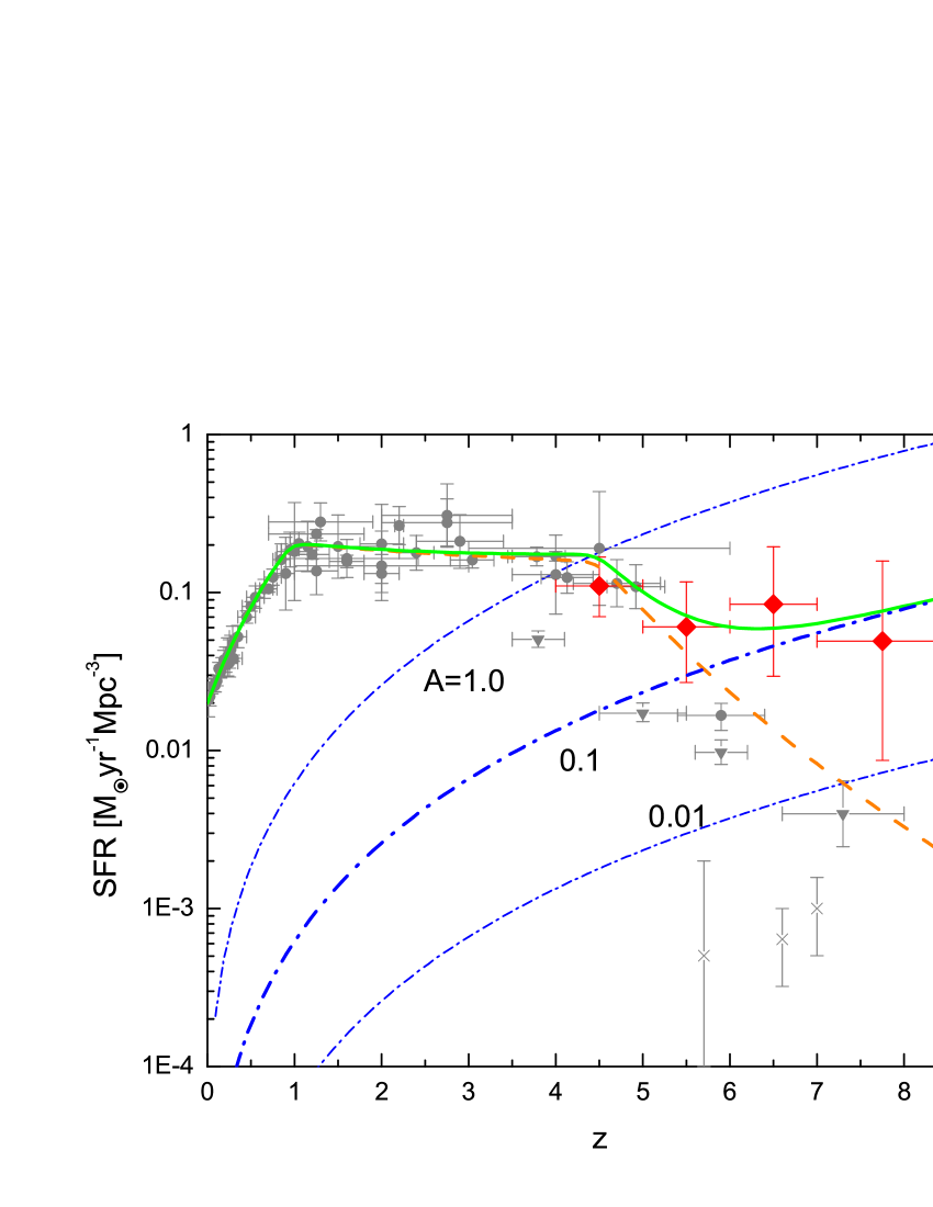
Figure 1: The cosmic star formation history. The SFR data (diamonds) inferred from the high-redshift GRBs Kis09 obviously deviate from the star formation history (dashed line) given by Ho06 , which is obtained by fitting the compiled SFR data inferred from galaxies (circles). For a comparison, we also exhibit the newer data inferred from the high-redshift Lyman break galaxies (triangles) Bou08 and Lyman-$\alpha$ emitters (crosses) ota08 . The dash-dotted lines represent the effective star formation history inferred from the CSGRBs with different values of $A$ and the solid line represents the combination of the dash and dash-dotted line for $A=0.1$.

Conclusion and discussions—The analysis in this Letter shows that all of the observed luminosities, durations, and event rate of high-redshift GRBs can be reasonably explained by ascribing some high-redshift GRBs to superconducting cosmic string bursts. Therefore, in the future SFR-determinations using high-redshift GRB sample, the possible pollution from CSGRBs must be eliminated carefully. In contrast to conventional GRBs, CSGRBs may have some unique features, e.g., a high luminosity accompanied by a very short duration, no association with supernova, and probably no host galaxy. More importantly, such an ascription inevitably suggests a new GRB original mechanism, in addition to the conventional progenitor models as collapsars and mergers of compact binaries. In other words, we can somewhat regard GRBs 080913 and 090423 as a new evidence for the existence of superconducting cosmic strings in the early Universe.

The superconducting cosmic string model may be tested in a variety of ways. First, as mentioned above, some high-frequency (e.g., GHz) electromagnetic waves directly radiated by a cusp at relatively low redshift can penetrate the surrounding medium and then be detected as a cosmic spark vac08 . Secondly, due to the quench of the current on the strings, superconducting cosmic strings could be a source for positrons, and thus the observed 511 keV emission from electron-positron annihilation in the Galactic bulge can be explained by the existence of a tangle of light superconducting strings in the Milky Wayfer05 . Thirdly, oscillating string loops can also contribute to gravitational wave (GW) background. The background spectrum has two main features, i.e., the “red noise” portion spanning the frequency range $10^{-8}$ Hz $\leq$ $f\leq 10^{10}$ Hz and the peak in the spectrum near $f\sim 10^{-12}$ Hz ViG . Gravitational waves in the frequency band $10^{-12}$ Hz $\leq f\leq 10^{-3}$ Hz produced by a cusp for string tensions as small as $G\mu/c^{2}\sim 10^{-10}$ could stand above the GW background Da , which might be detectable by the planned GW detectors such as LIGO, VIRGO, and LISA.

Finally, the ascription of some high-redshift GRBs to CSGRBs enables us to use high-redshift GRBs as a cosmological tool to constrain the primordial cosmic magnetic fields. At present, the magnetic fields on large scales are usually limited by the cosmic microwave background (CMB) and by Faraday rotation measures of light from high-redshift quasars. As a result, some upper limits (from $10^{-9}$ G to $10^{-7}$ G Ba ) for $B_{0}$ have been suggested. However, in view of the simplification of the CSGRB model and the smallness of the high-redshift GRB sample, the numerical results in this Letter are not yet sufficiently solid. Anyway, the CSGRB method at least provides a potentially effective complement to the CMB and the Faraday rotation methods. The combination of all these methods can give a more precise estimation on the strength of the primordial cosmic magnetic fields.

References

- (1) T. Piran, Rev. Mod. Phys. 76, 1143 (2005); P. Mészáros, Rept. Prog. Phys. 69, 2259 (2006); B. Zhang, Chin. J. Astron. Astrophys. 7, 1 (2007)
- (2) C. Kouveliotou et al., Astrophys. J. 413, L101 (1993).
- (3) J. Greiner et al., Astrophys. J. 693, 1610 (2009).
- (4) N. R. Tanvir et al., Nature 461, 1254 (2009); R. Salvaterra et al., Nature 461, 1258 (2009).
- (5) L. Amati et al., Astron. and Astrophys. 390, 81 (2002).
- (6) R.-R. Chary, E. Berger, and L. Cowie, Astrophys. J. 671, 272 (2007).
- (7) H. Yuksel, M. D. Kistler, J. F. Beacom, and A. M. Hopkins, Astrophys. J. 683, L5 (2008).
- (8) M. D. Kistler, H. Yuksel, J. F. Beacom, and K. Z. Stanek, Astrophys.J. 673, L119 (2008).
- (9) M. D. Kistler et al. Astrophys. J. 705, L104 (2009).
- (10) A. M. Hopkins and J. F. Beacom, Astrophys. J. 651, 142 (2006).
- (11) R. J. Bouwens, G. D. Illingworth, M. Franx, and H. Ford, Astrophys. J. 686, 230 (2008).
- (12) E. Witten, Nucl. Phys. B249, 557 (1985).
- (13) E. M. Chudnovsky, G. B. Field, D. N. Spergel, and A. Vilenkin, Phys. Rev. D34, 944 (1986); A. Vilenkin and T. Vachaspati, Phys. Rev. Lett. 58, 1041 (1987)
- (14) J. P. Ostriker, C. Thompson and E. Witten, Phys. Lett. B180, 231 (1986); D. N. Spergel, T. Piran and J. Goodman, Nucl. Phys. B291, 847 (1987); J.J. Blanco-Pillado, K. D. Olum and A. Vilenkin, Phys. Rev. D63, 103513 (2001).
- (15) D. R. Lormier, M. Bailes, M. A. McLaughlin, D. J. Narkevic, and F. Crawford, Science 318, 777 (2007).
- (16) T. Vachaspati, Phys. Rev. Lett. 101, 141301 (2008).
- (17) A. Babul, B. Paczynski, and D. Spergel, Astrophys. J. 316, L49 (1987).
- (18) B. Paczynski, Astrophys. J. 335, 525 (1988).
- (19) R. H. Brandenberger, A. T. Sornborger, and M. Trodden, Phys. Rev. D48, 940 (1993); R. Plaga, Astrophys. J. 424, L9 (1994).
- (20) V. Berezinsky, B. Hnatyk, and A. Vilenkin, Phys. Rev. D64, 043004 (2001); V. Berezinsky, B. Hnatyk, and A. Vilenkin, Baltic Astronomy 13, 289 (2004)
- (21) In the present Letter we consider the bolometric luminosity only. In more details, the spectral distribution of the released energy can be expressed by two asymptotic functions as for and for vac08 ; bla01 , where is the observational frequency, and Hz (see Equation 2) is the peak frequency of the spectrum. Since this peak frequency could be much lower than the plasma frequency of the surrounding medium vac08 , especially in the early Universe, we simply consider that nearly all of the total electromagnetic energy, as expressed by the bolometric luminosity, is absorbed by the interstellar medium to generate a GRB. Of course, by considering a possible decay of the loops due to the radiation effect (i.e., decreases), could increase to be above the plasma frequency. Therefore, at some relatively low redshifts, most energy may be released as an electromagnetic wave (e.g., radio) burst vac08 rather than to produce a GRB.
- (22) D. Ryu, H. Kang, and P. L. Biermann, Astron. Astrophys. 335, 19 (1998).
- (23) F. Ferrer and T. Vachaspati, Phys. Rev. Lett. 95, 261302 (2005).
- (24) A. Vilenkin, Phys. Lett. 107B, 47 (1981); R. R. Caldwell, R. A. Battye, and E. P. S. Shellard, Phys. Rev. D54, 7146 (1996).
- (25) T. Damour and A. Vilenkin, Phys. Rev. Lett. 85, 3761 (2000); T. Damour and A. Vilenkin, Phys. Rev. D 64, 064008 (2001); T. Damour and A. Vilenkin, Phys. Rev. D71, 063510 (2005).
- (26) J. D. Barrow, P. G. Ferreira, and J. Silk, Phys. Rev. Lett. 78, 3610 (1997); P. Blasi, S. Burles, and A.V. Olinto, Astrophys. J. Lett. 514, L79 (1999); R. Durrer, P. G. Ferreira, and T. Kahniashvili, Phys. Rev. D61, 043001 (2000).
- (27) K. Ota, et al., Astrophys. J. 677, 12
- (28) J. J. Vlanco-Pillado and Ken D. Olum, Nucl. Phys. B599, 435 (2001)