Non-local spin-sensitive electron transport in diffusive proximity heterostructures

Abstract

We formulate a quantitative theory of non-local electron transport in three-terminal disordered ferromagnet-superconductor-ferromagnet structures. We demonstrate that magnetic effects have different implications: While strong exchange field suppresses disorder-induced electron interference in ferromagnetic electrodes, spin-sensitive electron scattering at superconductor-ferromagnet interfaces can drive the total non-local conductance $g_{12}$ negative at sufficiently low energies. At higher energies magnetic effects become less important and the non-local resistance behaves similarly to the non-magnetic case. Our predictions can be directly tested in future experiments on non-local electron transport in hybrid $FSF$ structures.

I Introduction

The phenomenon of Andreev reflection (AR) And is well known to be responsible for transport of subgap electrons across an interface between a normal metal ($N$) and a superconductor ($S$). While this phenomenon is essentially local in hybrid proximity structures with only one $NS$ interface, the situation in multiterminal devices with two or more $NS$ interfaces (such as, e.g., $NSN$ structures) can be more complicated because in addition to local AR electrons can suffer non-local or crossed Andreev reflection (CAR) car . This phenomenon of CAR enables direct experimental demonstration of entanglement between electrons in spatially separated $N$-electrodes and can strongly influence non-local transport of electrons in hybrid $NSN$ systems FFH ; KZ06 .

Non-local electron transport in the presence of CAR was recently investigated both experimentally Beckmann ; Teun ; Venkat ; Basel ; Deutscher ; Beckmann2 and theoretically FFH ; KZ06 ; LY ; GZ09 ; BG ; Belzig ; Melin ; GZ07 ; Golubev09 ; Kalenkov07 ; Kalenkov07E demonstrating a rich variety of physical processes involved in the problem. For instance, the effect of CAR on the subgap non-local conductance of $NSN$ structures is exactly compensated by elastic cotunneling (EC) provided only the lowest order terms in $NS$ interface transmissions are accounted for FFH . Taking into account higher order processes in barrier transmissions eliminates this feature and yields non-zero values of cross-conductance KZ06 . One can also expect that interactions LY or external ac bias GZ09 can lift the cancellation between EC and CAR contributions already in the lowest order in barrier transmissions.

Another non-trivial issue is the effect of disorder. Theoretical analysis of CAR in different disordered $NSN$ structures was carried out in Refs. BG, ; Belzig, ; Melin, ; GZ07, ; Golubev09, . In particular, it was demonstrated Golubev09 that an interplay between CAR, quantum interference of electrons and non-local charge imbalance dominates the behavior of diffusive $NSN$ systems being essential for quantitative interpretation of a number of experimental observations Venkat ; Basel ; Deutscher .

Yet another important property of both local and non-local Andreev reflection processes is that they essentially depend on spins of scattered electrons. Hence, CAR should be sensitive to magnetic properties of normal electrodes. This sensitivity was indeed demonstrated already in the first experiments on ferromagnet-superconductor-ferromagnet ($FSF$) structures Beckmann where the dependence of non-local conductance on the polarization of ferromagnetic terminals was found. Theoretical analysis of spin-resolved CAR was carried out in Ref. FFH, in the lowest order order in tunneling and in Refs. Kalenkov07, , Kalenkov07E, to all orders in the interface transmissions. This analysis revealed a number of non-trivial features of non-local spin-dependent electron transport which can be tested in future experiments.

Note that previous work FFH ; Kalenkov07 ; Kalenkov07E merely concentrated on ballistic electrodes whereas in realistic experiments one usually deals with diffusive hybrid $FSF$ structures. Therefore it is highly desirable to formulate a theory which would adequately describe an interplay between disorder and spin-resolved CAR. This is the main goal of the present paper. The structure of our paper is as follows. In Sec. 2 we will formulate our model and outline our basic formalism of quasiclassical Green functions. This formalism will be employed in Sec. 3 where we present the solution of Usadel equations and derive general expressions for the non-local spin-dependent conductance and resistance for diffusive three-terminal $FSF$ structures at different directions of interface magnetizations. Concluding remarks are presented in Sec. 4 of our paper.

II Model and basic formalism

Let us consider a three-terminal diffusive $FSF$ structure schematically shown in Fig. 1. Two ferromagnetic terminals $F_{1}$ and $F_{2}$ with resistances $r_{N_{1}}$ and $r_{N_{2}}$ and electric potentials $V_{1}$ and $V_{2}$ are connected to a superconducting electrode of length $L$ with normal state (Drude) resistance $r_{L}$ and electric potential $V=0$ via tunnel barriers. The magnitude of the exchange field $h_{1,2}=|\bm{h}_{1,2}|$ in both ferromagnets $F_{1}$ and $F_{2}$ is assumed to be much bigger than the superconducting order parameter $\Delta$ of the $S$-terminal and, on the other hand, much smaller that the Fermi energy, i.e. $\Delta\ll h_{1,2}\ll\epsilon_{F}$.

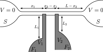
Figure 1: FSF structure under consideration.

The latter condition allows to perform the analysis of our $FSF$ system within the quasiclassical formalism of Usadel equations for the Green-Keldysh matrix functions $G$. In each of our metallic terminals these equations can be written in the form BWBSZ

$$iD\nabla(\check{G}\nabla\check{G})=[\check{\Omega}+eV,\check{G}],\quad\check{G}^{2}=1,$$ (1)

where $D$ is the diffusion constant, $V$ is the electric potential, $\check{G}$ and $\check{\Omega}$ are $8\times 8$ matrices in Keldysh-Nambu-spin space (denoted by check symbol)

$$\check{G}=\begin{pmatrix}\breve{G}^{R}&\breve{G}^{K}\\ 0&\breve{G}^{A}\\ \end{pmatrix},\quad\check{\Omega}=\begin{pmatrix}\breve{\Omega}^{R}&0\\ 0&\breve{\Omega}^{A}\\ \end{pmatrix},$$ (2)

$$\breve{\Omega}^{R}=\breve{\Omega}^{A}=\begin{pmatrix}\varepsilon-\hat{\bm{\sigma}}\bm{h}&\Delta\\ -\Delta^{*}&-\varepsilon+\hat{\bm{\sigma}}\bm{h}\\ \end{pmatrix},$$ (3)

$\varepsilon$ is the quasiparticle energy, $\Delta(T)$ is the superconducting order parameter which will be considered real in a superconductor and zero in both ferromagnets, $\bm{h}\equiv\bm{h}_{1(2)}$ in the first (second) ferromagnetic terminal, $\bm{h}\equiv 0$ outside these terminals and $\hat{\bm{\sigma}}=(\hat{\sigma}_{1},\hat{\sigma}_{2},\hat{\sigma}_{3})$ are Pauli matrices in spin space.

Retarded and advanced Green functions $\breve{G}^{R}$ and $\breve{G}^{A}$ have the following matrix structure

$$\breve{G}^{R,A}=\begin{pmatrix}\hat{G}^{R,A}&\hat{F}^{R,A}\\ -\hat{F}^{R,A}&-\hat{G}^{R,A}\\ \end{pmatrix}.$$ (4)

Here and below $2\times 2$ matrices in spin space are denoted by hat symbol.

Having obtained the expressions for the Green-Keldysh functions $\check{G}$ one can easily evaluate the current density $\bm{j}$ in our system with the aid of the standard relation

$$\bm{j}=-\frac{\sigma}{16e}\int\operatorname{\mathrm{Sp}}[\tau_{3}(\check{G}\nabla\check{G})^{K}]d\varepsilon,$$ (5)

where $\sigma$ is the Drude conductivity of the corresponding metal and $\tau_{3}$ is the Pauli matrix in Nambu space.

In what follows it will be convenient for us to employ the so-called Larkin-Ovchinnikov parameterization of the Keldysh Green function

$$\breve{G}^{K}=\breve{G}^{R}\breve{f}-\breve{f}\breve{G}^{A},\quad\breve{f}=\hat{f}_{L}+\tau_{3}\hat{f}_{T},$$ (6)

where the distribution functions $\hat{f}_{L}$ and $\hat{f}_{T}$ are $2\times 2$ matrices in the spin space.

For the sake of simplicity we will assume that magnetizations of both ferromagnets and the interfaces (see below) are collinear. Within this approximation the Green functions and the matrix $\check{\Omega}$ are diagonal in the spin space and the diffusion-like equations for the distribution function matrices $\hat{f}_{L}$ and $\hat{f}_{T}$ take the form

$$-D\nabla\left(\hat{D}^{T}(\bm{r},\varepsilon)\nabla\hat{f}_{T}(\bm{r},\varepsilon)\right)+2\hat{\Sigma}(\bm{r},\varepsilon)\hat{f}_{T}(\bm{r},\varepsilon)=0,$$ (7)

$$-D\nabla\left(\hat{D}^{L}(\bm{r},\varepsilon)\nabla\hat{f}_{L}(\bm{r},\varepsilon)\right)=0,$$ (8)

where

$$\hat{\Sigma}(\bm{r},\varepsilon)=-i\Delta\operatorname{\mathrm{Im}}\hat{F}^{R},$$ (9)

$$\hat{D}^{T}=\left(\operatorname{\mathrm{Re}}\hat{G}^{R}\right)^{2}+\left(\operatorname{\mathrm{Im}}\hat{F}^{R}\right)^{2},$$ (10)

$$\hat{D}^{L}=\left(\operatorname{\mathrm{Re}}\hat{G}^{R}\right)^{2}-\left(\operatorname{\mathrm{Re}}\hat{F}^{R}\right)^{2}.$$ (11)

The function $\hat{\Sigma}(\bm{r},\varepsilon)$ differs from zero only inside the superconductor. It accounts both for energy relaxation of quasiparticles and for their conversion to Cooper pairs due to Andreev reflection. The functions $\hat{D}^{T}$ and $\hat{D}^{L}$ acquire space and energy dependencies due to the presence of the superconducting wire and renormalize the diffusion coefficient $D$.

The solution of Eqs. (7)-(8) can be expressed in terms of the diffuson-like functions $\hat{\mathcal{D}}^{T}$ and $\hat{\mathcal{D}}^{L}$ which obey the following equations

$$\begin{split}-D\nabla\left[\hat{D}^{T}(\bm{r},\varepsilon)\nabla\hat{\mathcal{D}}^{T}(\bm{r},\bm{r}^{\prime},\varepsilon)\right]&\\ +2\hat{\Sigma}(\bm{r},\varepsilon)\hat{\mathcal{D}}^{T}(\bm{r},\bm{r}^{\prime},\varepsilon)=&\delta(\bm{r}-\bm{r}^{\prime}),\end{split}$$ (12)

$$-D\nabla\left[\hat{D}^{L}(\bm{r},\varepsilon)\nabla\hat{\mathcal{D}}^{L}(\bm{r},\bm{r}^{\prime},\varepsilon)\right]=\delta(\bm{r}-\bm{r}^{\prime}).$$ (13)

The solutions of Usadel equation (1) in each of the metals should be matched at $SF$-interfaces by means of appropriate boundary conditions which account for electron tunneling between these terminals. The form of these boundary conditions essentially depends on the adopted model describing electron scattering at $SF$-interfaces. Here we stick to the model of the so-called spin-active interfaces Eschrig which takes into account possibly different barrier transmissions for spin-up and spin-down electrons. This model was already extensively used for theoretical description of different physical phenomena, including spin-resolved CAR in ballistic structures Kalenkov07 ; Kalenkov07E and Josephson effect with triplet pairing Eschrig2 ; GKZ . Here we employ this model in the case of diffusive electrodes and also restrict our analysis to the case of tunnel barriers with channel transmissions much smaller than one. In this case the corresponding boundary conditions read Huertas02

$$\begin{split}\mathcal{A}\sigma_{+}&\check{G}_{+}\partial_{x}\check{G}_{+}=\dfrac{G_{T}}{2}[\check{G}_{-},\check{G}_{+}]\\ &+\dfrac{G_{m}}{4}[\{\hat{\bm{\sigma}}\bm{m}\tau_{3},\check{G}_{-}\},\check{G}_{+}]+i\dfrac{G_{\varphi}}{2}[\hat{\bm{\sigma}}\bm{m}\tau_{3},\check{G}_{+}],\end{split}$$ (14)

$$\begin{split}-\mathcal{A}&\sigma_{-}\check{G}_{-}\partial_{x}\check{G}_{-}=\dfrac{G_{T}}{2}[\check{G}_{+},\check{G}_{-}]\\ &+\dfrac{G_{m}}{4}[\{\hat{\bm{\sigma}}\bm{m}\tau_{3},\check{G}_{+}\},\check{G}_{-}]+i\dfrac{G_{\varphi}}{2}[\hat{\bm{\sigma}}\bm{m}\tau_{3},\check{G}_{-}],\end{split}$$ (15)

where $\check{G}_{-}$ and $\check{G}_{+}$ are the Green-Keldysh functions from the left ($x<0$) and from the right ($x>0$) side of the interface, $\mathcal{A}$ is the effective contact area, $\bm{m}$ is the unit vector in the direction of the interface magnetization, $\sigma_{\pm}$ are Drude conductivities of the left and right terminals and $G_{T}$ is the spin-independent part of the interface conductance. Along with $G_{T}$ there also exists the spin-sensitive contribution to the interface conductance which is accounted for by the $G_{m}$-term, whereas the $G_{\varphi}$-term arises due to different phase shifts acquired by scattered quasiparticles with opposite spin directions.

Employing the above boundary conditions we can establish the following linear relations between the distribution functions at both sides of the interface

$$\begin{split}\mathcal{A}\sigma_{+}\hat{D}_{+}^{T}&\partial_{x}\hat{f}_{+T}=\mathcal{A}\sigma_{-}\hat{D}_{-}^{T}\partial_{x}\hat{f}_{-T}\\ &=\hat{g}_{T}(\hat{f}_{+T}-\hat{f}_{-T})+\hat{g}_{m}(\hat{f}_{+L}-\hat{f}_{-L}),\end{split}$$ (16)

$$\begin{split}\mathcal{A}\sigma_{+}\hat{D}_{+}^{L}&\partial_{x}\hat{f}_{+L}=\mathcal{A}\sigma_{-}\hat{D}_{-}^{L}\partial_{x}\hat{f}_{-L}\\ &=\hat{g}_{L}(\hat{f}_{+L}-\hat{f}_{-L})+\hat{g}_{m}(\hat{f}_{+T}-\hat{f}_{-T}),\end{split}$$ (17)

where $\hat{g}_{T}$, $\hat{g}_{L}$, and $\hat{g}_{m}$ are matrix interface conductances which depend on the retarded and advanced Green functions at the interface

$$\hat{g}_{T}=G_{T}\left[\left(\operatorname{\mathrm{Re}}\hat{G}^{R}_{+}\right)\left(\operatorname{\mathrm{Re}}\hat{G}^{R}_{-}\right)+\left(\operatorname{\mathrm{Im}}\hat{F}^{R}_{+}\right)\left(\operatorname{\mathrm{Im}}\hat{F}^{R}_{-}\right)\right],$$ (18)

$$\hat{g}_{L}=G_{T}\left[\left(\operatorname{\mathrm{Re}}\hat{G}^{R}_{+}\right)\left(\operatorname{\mathrm{Re}}\hat{G}^{R}_{-}\right)-\left(\operatorname{\mathrm{Re}}\hat{F}^{R}_{+}\right)\left(\operatorname{\mathrm{Re}}\hat{F}^{R}_{-}\right)\right],$$ (19)

$$\hat{g}_{m}=G_{m}\hat{\bm{\sigma}}\bm{m}\left(\operatorname{\mathrm{Re}}\hat{G}^{R}_{+}\right)\left(\operatorname{\mathrm{Re}}\hat{G}^{R}_{-}\right).$$ (20)

The current density (5) can then be expressed in terms of the distribution function $\hat{f}_{T}$ as

$$\bm{j}=-\frac{\sigma}{4e}\int\operatorname{\mathrm{Sp}}[\hat{D}^{T}\nabla\hat{f}_{T}]d\varepsilon.$$ (21)

III Spectral conductances

Let us now employ the above formalism in order to evaluate electric currents in our $FSF$ device depicted in Fig. 1. The current across the first ($SF_{1}$) interface can be written as

$$I_{1}=\dfrac{1}{e}\int g_{11}(\varepsilon)\left[f_{0}(\varepsilon+eV_{1})-f_{0}(\varepsilon)\right]d\varepsilon\\ -\dfrac{1}{e}\int g_{12}(\varepsilon)\left[f_{0}(\varepsilon+eV_{2})-f_{0}(\varepsilon)\right]d\varepsilon,$$ (22)

where $f_{0}(\varepsilon)=\tanh(\varepsilon/2T)$, $g_{11}$ and $g_{12}$ are local and nonlocal spectral electric conductances. Expression for the current across the second interface can be obtained from the above equation by interchanging the indices $1\leftrightarrow 2$. Solving Eqs. (7)-(8) with boundary conditions (16)-(17) we express both local and nonlocal conductances $\hat{g}_{ij}(\varepsilon)$ in terms of the interface conductances and the function $\hat{\mathcal{D}}$. The corresponding results read

$$\begin{split}\hat{g}_{11}(\varepsilon)=\bigl{(}\hat{R}_{2}^{T}\hat{\mathcal{M}}^{L}+&\hat{R}_{2}^{T}\hat{R}_{2}^{L}\hat{R}_{1m}-\hat{R}_{1}^{L}\hat{R}_{2m}^{2}\\ +&\hat{R}_{12}^{T}\hat{R}_{12}^{L}\hat{R}_{2m}-\hat{R}_{1m}\hat{R}_{2m}^{2}\bigr{)}\hat{\mathcal{K}},\end{split}$$ (23)

$$\begin{split}\hat{g}_{12}(\varepsilon)=\hat{g}_{21}(\varepsilon)=\bigl{(}&\hat{R}_{12}^{T}\hat{\mathcal{M}}^{L}+\hat{R}_{2}^{T}\hat{R}_{12}^{L}\hat{R}_{1m}\\ +&\hat{R}_{12}^{L}\hat{R}_{1m}\hat{R}_{2m}+\hat{R}_{12}^{T}\hat{R}_{1}^{L}\hat{R}_{2m}\bigr{)}\hat{\mathcal{K}},\end{split}$$ (24)

where we defined

$$\hat{\mathcal{M}}^{T,L}=\hat{R}_{1}^{T,L}\hat{R}_{2}^{T,L}-(\hat{R}_{12}^{T,L})^{2},$$ (25)

$$\begin{split}\hat{\mathcal{K}}^{-1}=\hat{\mathcal{M}}^{T}\hat{\mathcal{M}}^{L}+&\hat{R}_{1m}^{2}\hat{R}_{2m}^{2}-\hat{R}_{2}^{T}\hat{R}_{2}^{L}\hat{R}_{1m}^{2}\\ -2&\hat{R}_{12}^{T}\hat{R}_{12}^{L}\hat{R}_{1m}\hat{R}_{2m}-\hat{R}_{1}^{T}\hat{R}_{1}^{L}\hat{R}_{2m}^{2}\end{split}$$ (26)

and introduced the auxiliary resistance matrix

$$\hat{R}_{1}^{T}=\hat{g}_{1T}(\varepsilon)[\hat{g}_{1T}(\varepsilon)\hat{g}_{1L}(\varepsilon)-\hat{g}_{1m}^{2}(\varepsilon)]^{-1}\\ +\dfrac{D_{1}\hat{\mathcal{D}}_{1}^{T}(\bm{r}_{1},\bm{r}_{1},\varepsilon)}{\sigma_{1}}+\dfrac{D_{S}\hat{\mathcal{D}}_{S}^{T}(\bm{r}_{1},\bm{r}_{1},\varepsilon)}{\sigma_{S}},$$ (27)

The resistance matrices $\hat{R}_{2}^{T}$, $\hat{R}_{1}^{L}$ and $\hat{R}_{2}^{L}$ can be obtained by interchanging the indices $1\leftrightarrow 2$ and $T\leftrightarrow L$ in Eq. (27). The remaining resistance matrices $\hat{R}_{12}^{T,L}$ and $\hat{R}_{jm}$ are defined as

$$\hat{R}_{12}^{T,L}=\hat{R}_{21}^{T,L}=\dfrac{D_{S}\hat{\mathcal{D}}_{S}^{T,L}(\bm{r}_{1},\bm{r}_{2},\varepsilon)}{\sigma_{S}},$$ (28)

$$\hat{R}_{jm}=\hat{g}_{jm}(\varepsilon)[\hat{g}_{jT}(\varepsilon)\hat{g}_{jL}(\varepsilon)-\hat{g}_{jm}^{2}(\varepsilon)]^{-1},$$ (29)

where $j=1,2$. The spectral conductance $g_{ij}$ can be recovered from the matrix $\hat{g}_{ij}$ simply by summing up over the spin states

$$g_{ij}(\varepsilon)=\dfrac{1}{2}\operatorname{\mathrm{Sp}}\left[\hat{g}_{ij}(\varepsilon)\right].$$ (30)

It is worth pointing out that Eqs. (23), (24) defining respectively local and nonlocal spectral conductances are presented with excess accuracy. This is because the boundary conditions (14)-(15) employed here remain applicable only in the tunneling limit and for weak spin dependent scattering $|G_{m}|,|G_{\varphi}|\ll G_{T}$. Hence, strictly speaking only the lowest order terms in $G_{m_{1,2}}$ and $G_{\varphi_{1,2}}$ need to be kept in our final results.

In order to proceed it is necessary to evaluate the interface conductances as well as the matrix functions $\hat{\mathcal{D}}^{T,L}_{1,2,S}$. Restricting ourselves to the second order in the interface transmissions we obtain

$$\hat{g}_{1T}(\varepsilon)=G_{T_{1}}\hat{\nu}_{S}(\bm{r}_{1},\varepsilon)+G_{T_{1}}^{2}\dfrac{\Delta^{2}\theta(\Delta^{2}-\varepsilon^{2})}{\Delta^{2}-\varepsilon^{2}}\hat{U}_{1}(\varepsilon),$$ (31)

$$\hat{g}_{1L}(\varepsilon)=G_{T_{1}}\hat{\nu}_{S}(\bm{r}_{1},\varepsilon)-G_{T_{1}}^{2}\dfrac{\Delta^{2}\theta(\varepsilon^{2}-\Delta^{2})}{\varepsilon^{2}-\Delta^{2}}\hat{U}_{1}(\varepsilon),$$ (32)

$$\hat{g}_{1m}(\varepsilon)=G_{m_{1}}\hat{\nu}_{S}(\bm{r}_{1},\varepsilon)\hat{\bm{\sigma}}\bm{m}_{1},$$ (33)

and analogous expressions for the interface conductances of the second interface. The matrix function

$$\hat{U}_{1}(\varepsilon)=\dfrac{D_{1}}{2\sigma_{1}}\Bigl{\{}\operatorname{\mathrm{Re}}\left[\mathcal{C}_{1}(\bm{r}_{1},\bm{r}_{1},2h_{1}^{+})+\mathcal{C}_{1}(\bm{r}_{1},\bm{r}_{1},2h_{1}^{-})\right]\\ -\hat{\bm{\sigma}}\bm{m}_{1}\operatorname{\mathrm{Re}}\left[\mathcal{C}_{1}(\bm{r}_{1},\bm{r}_{1},2h_{1}^{+})-\mathcal{C}_{1}(\bm{r}_{1},\bm{r}_{1},2h_{1}^{-})\right]\Bigr{\}}$$ (34)

with $h_{1}^{\pm}=h_{1}\pm\varepsilon$ defines the correction due to the proximity effect in the normal metal.

Taking into account the first order corrections in the interface transmissions one can derive the density of states inside the superconductor in the following form

$$\hat{\nu}_{S}(\bm{r},\varepsilon)=\dfrac{|\varepsilon|\theta(\varepsilon^{2}-\Delta^{2})}{\sqrt{|\varepsilon^{2}-\Delta^{2}|}}\\ +\dfrac{D_{S}}{\sigma_{S}}\dfrac{\Delta^{2}}{\Delta^{2}-\varepsilon^{2}}\sum_{i=1,2}\Biggl{[}G_{T_{i}}\operatorname{\mathrm{Re}}\mathcal{C}_{S}(\bm{r},\bm{r}_{i},2\omega^{R})\\ -\hat{\bm{\sigma}}\bm{m}_{i}G_{\varphi_{i}}\operatorname{\mathrm{Im}}\mathcal{C}_{S}(\bm{r},\bm{r}_{i},2\omega^{R})\Biggr{]},$$ (35)

where

$$\omega^{R}=\begin{cases}\sqrt{\varepsilon^{2}-\Delta^{2}},\quad&\varepsilon>\Delta,\\ i\sqrt{\Delta^{2}-\varepsilon^{2}},\quad&|\varepsilon|<\Delta,\\ -\sqrt{\varepsilon^{2}-\Delta^{2}},\quad&\varepsilon<\Delta,\end{cases}$$ (36)

and the Cooperon $\mathcal{C}_{j}(\bm{r},\bm{r}^{\prime},\varepsilon)$ represents the solution of the equation

$$\left(-D\nabla^{2}-i\varepsilon\right)\mathcal{C}(\bm{r},\bm{r}^{\prime},\varepsilon)=\delta(\bm{r}-\bm{r}^{\prime})$$ (37)

in the normal metal leads ($j=1,2$) and the superconductor ($j=S$). In the quasi-one-dimensional geometry the corresponding solutions take the form

$$\mathcal{C}_{j}(x_{j},x_{j},\varepsilon)=\dfrac{\tanh\left(k_{j}L_{j}\right)}{S_{j}D_{j}k_{j}},\quad j=1,2,$$ (38)

$$\mathcal{C}_{S}(x,x^{\prime},\varepsilon)=\dfrac{\sinh[k_{S}(L-x^{\prime})]\sinh k_{S}x}{k_{S}S_{S}D_{S}\sinh(k_{S}L)},\quad x^{\prime}>x,$$ (39)

where $S_{S,1,2}$ are the wire cross sections and $k_{1,2,S}=\sqrt{-i\varepsilon/D_{1,2,S}}$.

Substituting Eq. (35) into Eqs. (31) and (32) and comparing the terms $\propto G_{T_{1}}^{2}$ we observe that the tunneling correction to the density of states dominates over the terms proportional to $\hat{U}_{1}$ which contain an extra small factor $\sqrt{\Delta/h}\ll 1$. Hence, the latter terms in Eqs. (31) and (32) can be safely neglected. In addition, in Eq. (35) we also neglect small tunneling corrections to the superconducting density of states at energies exceeding the superconducting gap $\Delta$. Within this approximation the density of states inside the superconducting wire becomes spin-independent $\hat{\nu}_{S}(\bm{r},\varepsilon)=\hat{\sigma}_{0}\nu_{S}(\bm{r},\varepsilon)$. It can then be written as

$$\nu_{S}(\bm{r},\varepsilon)=\dfrac{|\varepsilon|}{\sqrt{|\varepsilon^{2}-\Delta^{2}|}}\theta(\varepsilon^{2}-\Delta^{2})\\ +\dfrac{D_{S}}{\sigma_{S}}\dfrac{\Delta^{2}\theta(\Delta^{2}-\varepsilon^{2})}{\Delta^{2}-\varepsilon^{2}}\sum\limits_{i=1,2}G_{T_{i}}\operatorname{\mathrm{Re}}\mathcal{C}_{S}(\bm{r},\bm{r}_{i},2\omega^{R}).$$ (40)

Accordingly, the interface conductances take the form

$$\hat{g}_{1T}(\varepsilon)=\hat{g}_{1L}(\varepsilon)=G_{T_{1}}\nu_{S}(\bm{r}_{1},\varepsilon),$$ (41)

$$\hat{g}_{1m}(\varepsilon)=G_{m_{1}}\nu_{S}(\bm{r}_{1},\varepsilon)\hat{\bm{\sigma}}\bm{m}_{1}.$$ (42)

In the limit of strong exchange fields $h_{1,2}\gg\Delta$ and small interface transmissions considered here the proximity effect in the ferromagnets remains weak and can be neglected. Hence, the functions $\hat{\mathcal{D}}^{T,L}_{1}(\bm{r}_{1},\bm{r}_{1},\varepsilon)$ and $\hat{\mathcal{D}}^{T,L}_{2}(\bm{r}_{2},\bm{r}_{2},\varepsilon)$ can be approximated by their normal state values

$$\hat{\mathcal{D}}^{T,L}_{1}(\bm{r}_{1},\bm{r}_{1},\varepsilon)=\sigma_{1}r_{N_{1}}\hat{1}/D_{1},$$ (43)

$$\hat{\mathcal{D}}^{T,L}_{2}(\bm{r}_{2},\bm{r}_{2},\varepsilon)=\sigma_{2}r_{N_{2}}\hat{1}/D_{2},$$ (44)

$$r_{N_{j}}=L_{j}/(\sigma_{j}S_{j}),\quad j=1,2,$$ (45)

where $r_{N_{1}}$ and $r_{N_{2}}$ are the normal state resistances of ferromagnetic terminals. In the the superconducting region an effective expansion parameter is $G_{T_{1,2}}r_{\xi_{S}}(\varepsilon)$, where $r_{\xi_{S}}(\varepsilon)=\xi_{S}(\varepsilon)/(\sigma_{S}S_{S})$ is the Drude resistance of the superconducting wire segment of length $\xi_{S}(\varepsilon)=\sqrt{D_{S}/2|\omega^{R}|}$. In the limit

$$G_{T_{1,2}}r_{\xi_{S}}(\varepsilon)\ll 1,$$ (46)

which is typically well satisfied for realistic system parameters, it suffices to evaluate the function $\hat{\mathcal{D}}^{T}_{S}(x,x^{\prime},\varepsilon)$ for impenetrable interfaces. In this case we find

$$\hat{\mathcal{D}}_{S}^{T}(x,x^{\prime},\varepsilon)=\begin{cases}\dfrac{\Delta^{2}-\varepsilon^{2}}{\Delta^{2}}\mathcal{C}_{S}(x,x^{\prime},2\omega^{R}),&|\varepsilon|<\Delta,\\ \dfrac{\varepsilon^{2}-\Delta^{2}}{\varepsilon^{2}}\mathcal{C}_{S}(x,x^{\prime},0),&|\varepsilon|>\Delta.\end{cases}$$ (47)

We note that special care should be taken while calculating $\mathcal{D}^{L}_{S}(x,x^{\prime},\varepsilon)$ at subgap energies, since the coefficient $D^{L}$ in Eq. (8) tends to zero deep inside the superconductor. Accordingly, the function $\mathcal{D}^{L}_{S}(x,x^{\prime},\varepsilon)$ becomes singular in this case. Nevertheless, the combinations $\hat{R}_{j}^{L}(\mathcal{M}^{L})^{-1}$ and $\hat{R}_{12}^{L}(\mathcal{M}^{L})^{-1}$ remain finite also in this limit. At subgap energies we obtain

$$\hat{R}_{1}^{L}(\hat{\mathcal{M}}^{L})^{-1}=\hat{R}_{2}^{L}(\hat{\mathcal{M}}^{L})^{-1}=\hat{R}_{12}^{L}(\hat{\mathcal{M}}^{L})^{-1}\\ =\dfrac{1}{r_{N_{1}}+r_{N_{2}}+\dfrac{2(\Delta^{2}-\varepsilon^{2})e^{d/\xi_{S}(\varepsilon)}}{\Delta^{2}r_{\xi_{S}}(\varepsilon)G_{T_{1}}G_{T_{2}}}},$$ (48)

where $d=|x_{2}-x_{1}|$ is the distance between two $SF$ contacts. Substituting the above relations into Eq. (24) we arrive at the final result for the non-local spectral conductance of our device at subgap energies

$$g_{12}(\varepsilon)=g_{21}(\varepsilon)=\dfrac{\Delta^{2}-\varepsilon^{2}}{\Delta^{2}}\dfrac{r_{\xi_{S}}(\varepsilon)\exp[-d/\xi_{S}(\varepsilon)]}{2[r_{N_{1}}+1/g_{T1}(\varepsilon)][r_{N_{2}}+1/g_{T2}(\varepsilon)]}\\ \times\left[1+\bm{m}_{1}\bm{m}_{2}\dfrac{G_{m1}}{g_{T1}(\varepsilon)}\dfrac{G_{m2}}{g_{T2}(\varepsilon)}\dfrac{\Delta^{2}}{\Delta^{2}-\varepsilon^{2}}\dfrac{1}{1-\dfrac{\varepsilon^{2}}{\Delta^{2}}+\dfrac{r_{N_{1}}+r_{N_{2}}}{2}r_{\xi_{S}}(\varepsilon)G_{T_{1}}G_{T_{2}}\exp[-d/\xi_{S}(\varepsilon)]}\right],\quad|\varepsilon|<\Delta.$$ (49)

Eq. (49) represents the central result of our paper. It consists of two different contributions. The first of them is independent of the interface polarizations $\bm{m}_{1,2}$. This term represents direct generalization of the result Golubev09 in two different aspects. Firstly, the analysis Golubev09 was carried out under the assumption $r_{N_{1,2}}g_{T1,2}(\varepsilon)\ll 1$ which is abandoned here. Secondly (and more importantly), sufficiently large exchange fields $h_{1,2}\gg\Delta$ of ferromagnetic electrodes suppress disorder-induced electron interference in these electrodes and, hence, eliminate the corresponding zero-bias anomaly both in local VZK ; HN ; Z and non-local Golubev09 spectral conductances. In this case with sufficient accuracy one can set $g_{Ti}(\varepsilon)=G_{Ti}\nu_{S}(x_{i},\varepsilon)$ implying that at subgap energies $g_{Ti}(\varepsilon)$ is entirely determined by the second term in Eq. (40) which yields in the case of quasi-one-dimensional electrodes

$$g_{T1}(\varepsilon)=\dfrac{\Delta^{2}G_{T_{1}}r_{\xi_{S}}(\varepsilon)}{2(\Delta^{2}-\varepsilon^{2})}\left[G_{T_{1}}+G_{T_{2}}e^{-d/\xi_{S}(\varepsilon)}\right],$$ (50)

$$g_{T2}(\varepsilon)=\dfrac{\Delta^{2}G_{T_{2}}r_{\xi_{S}}(\varepsilon)}{2(\Delta^{2}-\varepsilon^{2})}\left[G_{T_{2}}+G_{T_{1}}e^{-d/\xi_{S}(\varepsilon)}\right].$$ (51)

Note, that if the exchange field $h_{1,2}$ in both normal electrodes is reduced well below $\Delta$ and eventually is set equal to zero, the term containing $\hat{U}_{1}(\varepsilon)$ in Eqs. (31), (32) becomes important and should be taken into account. In this case we again recover the zero-bias anomaly VZK ; HN ; Z $g_{Ti}(\varepsilon)\propto 1/\sqrt{\varepsilon}$ and from the first term in Eq. (49) we reproduce the results Golubev09 derived in the limit $h_{1,2}\to 0$.

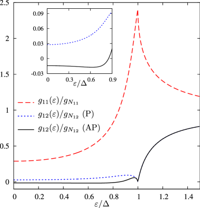
Figure 2: (Color online) Local (long-dashed line) and non-local (short-dashed and solid lines) spectral conductances normalized to its normal state values. Here we choose $r_{N_{1}}=r_{N_{2}}=5r_{\xi_{S}}(0)$, $x_{1}=L-x_{2}=5\xi_{S}(0)$, $x_{2}-x_{1}=\xi_{S}(0)$, $G_{T_{1}}=G_{T_{2}}=4G_{m_{1}}=4G_{m_{2}}=0.2/r_{\xi_{S}}(0)$. Energy dependence of non-local conductance is displayed for parallel (P) $\bm{m}_{1}\bm{m}_{2}=1$ and antiparallel (AP) $\bm{m}_{1}\bm{m}_{2}=-1$ interface magnetizations. Inset: The same in the limit of low energies.

The second term in Eq. (49) is proportional to the product $\bm{m}_{1}\bm{m}_{2}G_{m1}G_{m2}$ and describes non-local magnetoconductance effect in our system emerging due to spin-sensitive electron scattering at $SF$ interfaces. It is important that – despite the strong inequality $|G_{mi}|\ll G_{Ti}$ – both terms in Eq. (49) can be of the same order, i.e. the second (magnetic) contribution can significantly modify the non-local conductance of our device.

In the limit of large interface resistances $r_{N_{1,2}}g_{T1,2}(\varepsilon)\ll 1$ the formula (49) reduces to a much simpler one

$$g_{12}(\varepsilon)=g_{21}(\varepsilon)=\dfrac{r_{\xi_{S}}(\varepsilon)}{2}\exp[-d/\xi_{S}(\varepsilon)]\\ \times\left[\dfrac{\Delta^{2}-\varepsilon^{2}}{\Delta^{2}}g_{T1}(\varepsilon)g_{T2}(\varepsilon)+\bm{m}_{1}\bm{m}_{2}G_{m1}G_{m2}\dfrac{\Delta^{2}}{\Delta^{2}-\varepsilon^{2}}\right].$$ (52)

Interestingly, Eq. (52) remains applicable for arbitrary values of the angle between interface polarizations $\bm{m}_{1}$ and $\bm{m}_{2}$ and strongly resembles the analogous result for the non-local conductance in ballistic $FSF$ systems (cf., e.g., Eq. (77) in Ref. Kalenkov07, ). The first term in the square brackets in Eq. (52) describes the fourth order contribution in the interface transmissions which remains nonzero also in the limit of the nonferromagnetic leads Golubev09 . In contrast, the second term is proportional to the product of transmissions of both interfaces, i.e. only to the second order in barrier transmissions FFH ; Kalenkov07 . This term vanishes identically provided at least one of the interfaces is spin-isotropic.

Contrary to the non-local conductance at subgap energies, both local conductance (at all energies) and non-local spectral conductance at energies above the superconducting gap are only weakly affected by magnetic effects. Neglecting small corrections due to $G_{m}$ term in the boundary conditions we obtain

$$\hat{g}_{11}(\varepsilon)=\hat{R}_{1}^{T}(\hat{\mathcal{M}}^{T})^{-1},\quad\hat{g}_{22}(\varepsilon)=\hat{R}_{2}^{T}(\hat{\mathcal{M}}^{T})^{-1},$$ (53)

$$\hat{g}_{12}(\varepsilon)=g_{21}(\varepsilon)=\hat{R}_{12}^{T}(\hat{\mathcal{M}}^{T})^{-1},\quad|\varepsilon|>\Delta.$$ (54)

Eqs. (53) and (54) together with the above expressions for the non-local subgap conductance enable one to recover both local and non-local spectral conductances of our system at all energies. Typical energy dependencies for both $g_{11}(\varepsilon)$ and $g_{12}(\varepsilon)$ are displayed in Fig. 2. For instance, we observe that at subgap energies the non-local conductance $g_{12}$ changes its sign being positive for parallel and negative for antiparallel interface polarizations.

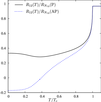
Figure 3: (Color online) Non-local resistance (normalized to its normal state value) versus temperature (normalized to the superconducting critical temperature $T_{C}$) for parallel (P) and antiparallel (AP) interface magnetizations. The parameters are the same as in Fig. 2.

Figure 4: (Color online) The same as in Fig. 3 for the following parameter values: $r_{N_{1}}=r_{N_{2}}=5r_{\xi_{S}}(0)$, $x_{1}=L-x_{2}=5\xi_{S}(0)$, $x_{2}-x_{1}=\xi_{S}(0)$, $G_{T_{1}}=G_{T_{2}}=50G_{m_{1}}=50G_{m_{2}}=0.025/r_{\xi_{S}}(0)$.

Having established the spectral conductance matrix $g_{ij}(\varepsilon)$ one can easily recover the complete $I-V$ curves for our hybrid $FSF$ structure. In the limit of low bias voltages these $I-V$ characteristics become linear, i.e.

$$I_{1}=G_{11}(T)V_{1}+G_{12}(T)V_{2},$$ (55)

$$I_{2}=G_{21}(T)V_{1}+G_{22}(T)V_{2},$$ (56)

where $G_{ij}(T)$ represent the linear conductance matrix defined as

$$G_{ij}(T)=\dfrac{1}{4T}\int g_{ij}(\varepsilon)\dfrac{d\varepsilon}{\cosh^{2}\dfrac{\varepsilon}{2T}}.$$ (57)

It may also be convenient to invert the relations (55)-(56) thus expressing induced voltages $V_{1,2}$ in terms of injected currents $I_{1,2}$:

$$V_{1}=R_{11}(T)I_{1}-R_{12}(T)I_{2},$$ (58)

$$V_{2}=-R_{21}(T)I_{1}+R_{22}(T)I_{2},$$ (59)

where the coefficients $R_{ij}(T)$ define local ($i=j$) and nonlocal ($i\neq j$) resistances

$$R_{11}(T)=\dfrac{G_{22}(T)}{G_{11}(T)G_{22}(T)-G_{12}^{2}(T)},$$ (60)

$$R_{12}(T)=R_{21}(T)=\dfrac{G_{12}(T)}{G_{11}(T)G_{22}(T)-G_{12}^{2}(T)}$$ (61)

and similarly for $R_{22}(T)$. In non-ferromagnetic $NSN$ structures the low temperature non-local resistance $R_{12}(T\to 0)$ turns out to be independent of both the interface conductances and the parameters of the normal leads Golubev09 . However, this universality of $R_{12}$ does not hold anymore provided non-magnetic normal metal leads are substituted by ferromagnets. Non-local linear resistance $R_{12}$ of our $FSF$ structure is displayed in Figs. 3, 4 as a function of temperature for parallel ($\bm{m}_{1}\bm{m}_{2}=1$) and antiparallel ($\bm{m}_{1}\bm{m}_{2}=-1$) interface magnetizations. In Fig. 3 we show typical temperature behavior of the non-local resistance for sufficiently transparent interfaces. For both mutual interface magnetizations $R_{12}$ first decreases with temperature below $T_{C}$ similarly to the non-magnetic case. However, at lower $T$ important differences occur: While in the case of parallel magnetizations $R_{12}$ always remains positive and even shows a noticeable upturn at sufficiently low $T$, the non-local resistance for antiparallel magnetizations keeps monotonously decreasing with $T$ and may become negative in the low temperature limit. In the limit of very low interface transmissions the temperature dependence of the non-local resistance exhibits a well pronounced charge imbalance peak (see Fig. 4) which physics is similar to that analyzed in the case of non-ferromagnetic $NSN$ structures KZ06 ; GZ07 ; GKZ . Let us point out that the above behavior of the non-local resistance is qualitatively consistent with available experimental observations Beckmann .

IV Concluding remarks

In this paper we developed a quantitative theory of non-local electron transport in three-terminal hybrid ferromagnet-superconductor-ferromagnet structures in the presence of disorder in the electrodes. Within our model transfer of electrons across $SF$ interfaces is described in the tunneling limit and magnetic properties of the system are accounted for by introducing ($i$) exchange fields $\bm{h}_{1,2}$ in both normal metal electrodes and ($ii$) magnetizations $\bm{m}_{1,2}$ of both $SF$ interfaces (the model of spin-active interfaces). The two ingredients ($i$) and ($ii$) of our model are in general independent from each other and have different physical implications. While the role of (comparatively large) exchange fields $h_{1,2}\gg\Delta$ is merely to suppress disorder-induced interference of electrons VZK ; HN ; Z penetrating from a superconductor into ferromagnetic electrodes, spin-sensitive electron scattering at $SF$ interfaces yields an extra contribution to the non-local conductance which essentially depends on relative orientations of the interface magnetizations. For anti-parallel magnetizations the total non-local conductance $g_{12}$ and resistance $R_{12}$ can turn negative at sufficiently low energies/temperatures. At higher temperatures the difference between the values of $R_{12}$ evaluated for parallel and anti-parallel magnetizations becomes less important. At such temperatures the non-local resistance behaves similarly to the non-magnetic case demonstrating, e.g., a well-pronounced charge imbalance peak GKZ in the limit of low interface transmissions.

We believe that our predictions can be directly used for quantitative analysis of future experiments on non-local electron transport in hybrid $FSF$ structures.

Acknowledgments

This work was supported in part by DFG and by RFBR grant 09-02-00886. M.S.K. also acknowledges support from the Council for grants of the Russian President (Grant No. 89.2009.2) and from the Dynasty Foundation.

References

- (1) A.F. Andreev, Sov. Phys. JETP 19, 1228 (1964).
- (2) J.M. Byers and M.E. Flatte, Phys. Rev. Lett. 74, 306 (1995); G. Deutscher and D. Feinberg, Appl. Phys. Lett. 76, 487 (2000).
- (3) G. Falci, D. Feinberg, and F.W.J. Hekking, Europhys. Lett. 54, 255 (2001).
- (4) M.S. Kalenkov and A.D. Zaikin, Phys. Rev. B 75, 172503 (2007); JETP Lett. 87, 140 (2008).
- (5) D. Beckmann, H.B. Weber, and H. v. Löhneysen, Phys. Rev. Lett. 93, 197003 (2004).
- (6) S. Russo, M. Kroug, T.M. Klapwijk, and A.F. Morpurgo, Phys. Rev. Lett. 95, 027002 (2005).
- (7) P. Cadden-Zimansky and V. Chandrasekhar, Phys. Rev. Lett. 97, 237003 (2006); P. Cadden-Zimansky, Z. Jiang, and V. Chandrasekhar, New J. Phys. 9, 116 (2007).
- (8) A. Kleine, A. Baumgartner, J. Trbovic, and C. Schönenberger, Europhys. Lett. 87, 27011 (2009); A. Kleine, A. Baumgartner, J. Trbovic, D.S. Golubev, A.D. Zaikin, and C. Schönenberger, arXiv:0911.4427 (2009).
- (9) B. Almog, S. Hacohen-Gourgy, A. Tsukernik, and G. Deutscher, Phys. Rev. B 80, 220512(R) (2009).
- (10) J. Brauer, F. Hübler, M. Smetanin, D. Beckmann, and H. v. Löhneysen, Phys. Rev. B 81, 024515 (2010).
- (11) A. Levy Yeyati, F.S. Bergeret, A. Martin-Rodero, and T.M. Klapwijk, Nat. Phys. 3, 455 (2007).
- (12) D.S. Golubev and A.D. Zaikin, Europhys. Lett. 86, 37009 (2009).
- (13) A. Brinkman and A.A. Golubov, Phys. Rev. B 74, 214512 (2006).
- (14) J.P. Morten, A. Brataas, and W. Belzig, Phys. Rev. B 74, 214510 (2006).
- (15) R. Melin, Phys. Rev. B 73, 174512 (2006).
- (16) D.S. Golubev and A.D. Zaikin, Phys. Rev. B 76, 184510 (2007).
- (17) D.S. Golubev, M.S. Kalenkov, and A.D. Zaikin, Phys. Rev. Lett. 103, 067006 (2009).
- (18) M.S. Kalenkov and A.D. Zaikin, Phys. Rev. B 76, 224506 (2007).
- (19) M.S. Kalenkov and A.D. Zaikin, Physica E 40, 147 (2007).
- (20) See, e.g., W. Belzig, F. Wilhelm, C. Bruder, G. Schön, and A.D. Zaikin, Superlatt. Microstruct. 25, 1251 (1999).
- (21) M. Eschrig, Phys. Rev. B 80, 134511 (2009).
- (22) M. Eschrig, J. Kopu, J. C. Cuevas, and G. Schön, Phys. Rev. Lett. 90, 137003 (2003); M. Eschrig and T. Lofwander, Nat. Phys. 4, 138 (2008).
- (23) A.V. Galaktionov, M.S. Kalenkov, and A.D. Zaikin, Phys. Rev. B 77, 094520 (2008); M.S. Kalenkov, A.V. Galaktionov, and A.D. Zaikin, Phys. Rev. B 79, 014521 (2009).
- (24) D. Huertas-Hernando, Yu.V. Nazarov, and W. Belzig, Phys. Rev. Lett. 88, 047003 (2002); A. Cottet, D. Huertas-Hernando, W. Belzig, and Yu.V. Nazarov, Phys. Rev. B 80, 184511 (2009).
- (25) A.F. Volkov, A.V. Zaitsev, and T.M. Klapwijk, Physica C 210, 21 (1993).
- (26) F.W.J. Hekking and Yu.V. Nazarov, Phys. Rev. Lett. 71, 1625 (1993).
- (27) A.D. Zaikin, Physica B 203, 255 (1994).