Giant Planet Occurrence in the Stellar Mass-Metallicity Plane

Abstract

Correlations between stellar properties and the occurrence rate of exoplanets can be used to inform the target selection of future planet search efforts and provide valuable clues about the planet formation process. We analyze a sample of 1266 stars drawn from the California Planet Survey targets to determine the empirical functional form describing the likelihood of a star harboring a giant planet as a function of its mass and metallicity. Our stellar sample ranges from M dwarfs with masses as low as 0.2 M_⊙ to intermediate-mass subgiants with masses as high as 1.9 M_⊙. In agreement with previous studies, our sample exhibits a planet-metallicity correlation at all stellar masses; the fraction of stars that harbor giant planets scales as $f\propto 10^{1.2\rm[Fe/H]}$. We can rule out a flat metallicity relationship among our evolved stars (at 98% confidence), which argues that the high metallicities of stars with planets is not likely due to convective envelope “pollution.” Our data also rule out a constant planet occurrence rate for [Fe/H] $<0$, indicating that giant planets continue to become rarer at sub-Solar metallicities. We also find that planet occurrence increases with stellar mass ($f\propto M_{\star}$), characterized by a rise from 3% around M dwarfs (0.5 M_⊙) to 14% around A stars (2 M_⊙), at Solar metallicity. We argue that the correlation between stellar properties and giant planet occurrence is strong supporting evidence of the core accretion model of planet formation.

1. Introduction

Mass and chemical composition are key quantities in the formation, evolution and fate of stars. A star of a given age is, to first order, characterized by these two physical parameters, and the influences of mass and metallicity extend to the formation and evolution of planets (johnson09rev). Even the first handful of exoplanet discoveries revealed that the likelihood of a star harboring a planet was closely tied to stellar iron content, or metallicity [Fe/H] (gonzalez97). Subsequent studies of larger samples of stars using uniform spectroscopic modeling techniques found that giant planet occurrence increases sharply for stellar metallicity in excess of the Solar value, rising from 3% for [Fe/H] $\lesssim 0$ to 25% for [Fe/H] $>+0.4$ (santos04; fischer05b, hereafter FV05).

In addition to informing models of planet formation (ida05a; mordasini09; johansen09), the planet-metallicity correlation (PMC) has provided a guide for the target selection of subsequent planet searches. The Next 2000 Stars (N2K) and Metallicity-Biased CORALIE surveys leveraged the higher metallicities of their samples to detect large numbers of close-in planets, many of which transit their host stars and thereby yield key insights into the interior structures of Jovian exoplanets (fischer05a; bouchy05; johnson06; moutou06). Indeed, studies of known transiting planets have revealed evidence of a correlation between planetary core mass and the metallicity of their host stars (sato05; torres08; guillot06; burrows07c).

While the first planet detections yielded a definitive correlation between giant planet occurrence and stellar metallicity, until recently very little was known about the effects of stellar mass (laws03). The first Doppler-based planet surveys concentrated primarily on stars with masses similar to the Sun, both because it was desirable to find Solar System analogs and because Sun-like stars make excellent planet-search targets. Compared to more massive stars, dwarfs with masses within $1.0\pm 0.2$ M_⊙ are relatively numerous, have cool atmospheres and slow rotational velocities ($V_{\rm rot}\sin{i}$ $\lesssim 5$ km s^-1). The latter two features result in a high density of narrow absorption lines in the spectra of Sun-like stars, which is ideal measuring for stellar Doppler shifts to high precision.

Stars at the lower end of the mass scale (the K and M stars) are even more numerous than the Sun and they also display large number of narrow absorption features in their spectra. However, most low-mass stars are optically faint ($V_{mag}\gtrsim 10$) and are thus not included in large numbers in most Doppler surveys. The faintness of late-K and M-type dwarfs can be overcome by using larger telescopes (butler04; bonfils05b), and more recently by observing at infrared wavelengths (bean10). Despite the small numbers of M dwarfs thus far monitored by Doppler surveys, one result has become apparent: M dwarfs harbor Jovian planets very infrequently. Only eight systems containing one or more giant planets have been found among the $\approx 300$ M dwarfs on various Doppler programs (johnson10a; nader10).

It was originally thought that the paucity of Jupiter-mass planets around M dwarfs was due to a metallicity bias among nearby, low-mass stars (bonfils05a). However, a recent study by johnson09b revealed that M dwarfs likely have the same metallicity distribution as Sun-like stars, and stars with masses $M_{\star}<0.5$ M_⊙ are 2-4 times less likely than Sun-like stars to have a Jupiter (johnson07b; johnson10a).

At the other end of the mass scale, the problems inherent to massive, early-type stars can be overcome by observing targets at a later stage of their evolution (hatzes03; setiawan05; sato05; reffert06; johnson07; nied07; liu08; dollinger09). Once stars exhaust their core hydrogen fuel sources they move off of the main sequence, become cooler, and shed a large fraction of their primordial angular momentum (gray85; donascimento00). The effects of stellar evolution transform a 2 M_⊙ star from an A-type dwarf with $V_{\rm rot}\sin{i}$ $\sim 100$ km s^-1 and $T_{\rm eff}$ $=8200$ K, to a K-type subgiant or giant with $V_{\rm rot}\sin{i}$ $<2$ km s^-1 and $T_{\rm eff}$ $\approx 4800$ K (demedeiros97; girardi02; sandage03). Surveys of “retired” massive stars have resulted in the discovery of $\approx 30$ Jupiter-mass planets with well-characterized orbits (see e.g. Table 1 of bowler10).

Using a sample of stars spanning a wide range of masses, johnson07b measured a positive correlation between stellar mass and the fraction of stars with detectable planets. In a related study, bowler10 measured a planet occurrence rate of $26^{+9}_{-8}$% among a uniform sample of 31 massive subgiants. Furthermore, based in part on a study of planets around K giants in nearby open clusters, lovis07 found that the average planet mass increases as a function of stellar mass, indicating that gas giant planets become either more massive on average, or more numerous (or both) with increasing stellar mass (see also bowler10).

The observed correlation between stellar mass and the occurrence of detectable planets, like the PMC before it, has added an important new variable to models of planet formation. While the Sun and Solar-mass stars serve as important benchmarks for understanding the formation of our own planetary system, successful, generalized planet formation theories must now account for the effects of stellar mass, and presumably by extension, disk mass (laughlin04; ida05a; kennedy08; currie09).

While previous studies have uncovered the existence of a positive correlation between stellar mass and planet occurrence, it is important to understand the underlying functional form of the relationship. For example, it would be advantageous to know whether the correlation is purely linear, or if it can instead be better described as some other functional form. Besides informing theories of planet formation, an improved understanding of the relationship between planet occurrence and stellar mass will also help guide the target selection of future surveys, and aid in the interpretation of results of current and future planet-search efforts. Just as some previous Doppler surveys biased their target selection toward high-metallicity stars to increase their yield, future direct-imaging, astrometric and Doppler surveys may benefit from concentrating on more massive stars. This strategy has paid off for one high-contrast imaging survey, resulting in the detection of three giant planets around the A5 dwarf HR 8799 (marois08). Another example of an imaged planet is Fomalhaut b, which is a giant planet ($\lesssim 3.3$ $M_{\rm Jup}$) orbiting just inside of a debris disk of an A3V star (kalas08; chiang09). Even in the cases when surveys do not yield detections, proper interpretation of null results requires knowledge of the expected number of detections (e.g. nielsen09).

Ascertaining the underlying form of the dependence of giant planet occurrence on stellar mass requires a larger sample than used in previous studies. Since the publication of johnson07b a sample of 240 new intermediate-mass subgiants have been added to the California Planet Survey (CPS) at Keck Observatory johnson10b. At the low-mass end, two new giant planets have been discovered among the CPS Keck sample of M dwarfs (johnson10a). Improvements in our ability to estimate the metallicities of M dwarfs and massive evolved stars have provided vital information about how to properly isolate the effects of stellar mass from the known effects of stellar metallicity. With these tools at hand, we are now poised to make an updated evaluation of the relationship between stellar mass and planet occurrence.

Our paper is organized as follows. In § 2 we present the characteristics of our three primary samples, including low-mass M dwarfs from Keck observatory; “Sun-like” late-F, G and K (FGK) dwarfs from the main CPS sample; and massive, evolved stars from the Lick and Keck subgiant surveys. In § 3 we examine the separate effects of mass and metallicity on planet occurrence. In § 4 we present our Bayesian inference technique of measuring correlations between planet occurrence and stellar characteristics and we provide the best-fitting parameters for the measured relationship in § 5. We compare our results with previous work in § 6. Finally, we summarize our key results and discuss our findings in the context of the current theoretical understanding of planet formation in § 7.

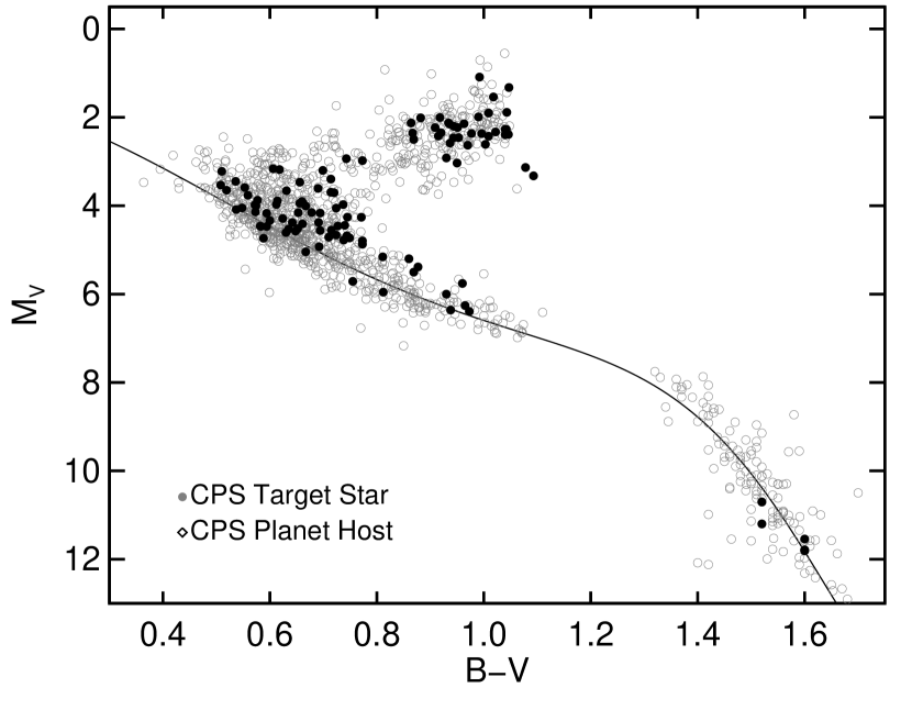
Figure 1.— H-R diagram showing our stellar sample (filled circles) and planet host stars (open circles). The solid line is the polynomial relationship describing the mean Hipparcos main sequence wright04. The excess scatter seen about the lower main sequence $B-V>1.2$ is primarily due to errors in the published V-band magnitudes and/or parallaxes for those faint stars.

2. Selection of Stars and Planets

Our goal is to measure planet occurrence as a function of stellar properties. Care must be exercised in selecting the sample of target stars such that planets of a given mass and orbital semimajor axis could be uniformly detected over the entire sample. The criteria for planet mass and semimajor axis translate into limits on velocity amplitudes, $K$, and orbital periods that can be tallied among the sample of planet detections. These criteria must be selected to ensure reasonably uniform detection characteristics across several Doppler surveys, which have different detection sensitivities and time baselines.

In what follows, we describe our selection of stars and planets from among the various CPS planet search programs. The CPS is a collection of Doppler surveys carried out primarily at the Lick and Keck Observatories. The CPS target lists provide a large stellar sample with a wide range of masses and metallicities. Specifically, our stars lie in the ranges $0.2<M_{\star}/M_{\odot}\lesssim 2.0$ and $-1.0<$ [Fe/H] $<+0.55$. The long time baselines ranging from 3 to 10 years, and Doppler precision ranging from 1–5 m s^-1 have resulted in a diverse and fairly complete sample of giant planets that have been compiled in the Catalog of Nearby Exoplanets (CNE, butler06) as updated by Wright et al. 2010 (in prep) in the Exoplanet Orbit Database.

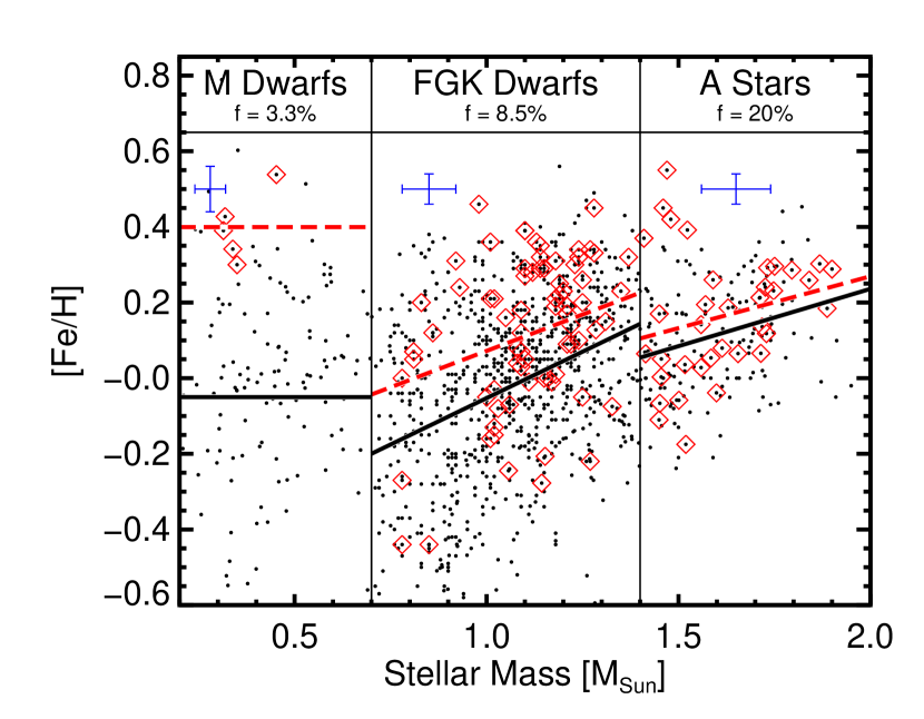
Figure 2.— A plot of stellar mass ($M_{\star}$) and metallicity ([Fe/H]) for the full stellar sample, comprised of 1194 stars (black dots), 115 of which harbor at least one detectable planet (red diamonds). For visualization, we have divided the stellar sample into three broad groups: M dwarfs, FGK dwarfs, and massive “retired” A stars. The fraction $f$ of stars with planets is printed above each group. The thick (black) lines each stellar mass group represent the best-fitting linear relationships between mass and metallicity (for the M dwarfs the lines represent the metallicity). The dashed (red) line is the best-fitting linear relationship between mass and metallicity for the stars with planets. For the M dwarfs we simply report the average metallicity for each population. The (blue) 2-dimensional error bars represent the typical measurement uncertainties. In each mass group, there is a systematic metallicity offset between the stars with and without planets. Discontinuities between the samples are not entirely physical, and are in large part due to the different target-selection criteria for the three surveys.

2.1. Stellar Sample

The low-mass stars in our sample are drawn from from the CPS Keck survey of late-K and M-type dwarfs (rauscher06; johnson10a). This sample comprises stars with $M_{\star}<0.6$ M_⊙ as estimated with the photometric calibration of delfosse00. We estimate the metallicities with the broadband photometric calibration of johnson09b, which relates the metallicity of a star to its “height” ($\Delta M_{K}$) above the mean main-sequence in the $\{V-K_{S}$, $M_{K_{S}}\}$ plane.

The bulk of our Solar-mass F, G and K dwarfs are taken from the Spectroscopic Properties of Cool Stars catalog (SPOCS; valenti05). Most of these stars have masses in the range $0.8<M_{\star}/M_{\sun}<1.2$. However, the SPOCS catalog contains some higher mass subgiants, which we fold into our high-mass stellar sample described herein. The spectroscopic properties listed in the SPOCS catalog were measured using the LTE spectral synthesis software package Spectroscopy Made Easy (SME; valenti96), as described by valenti05 and FV05. Stellar masses for the SPOCS catalog are cataloged by takeda07, who associate the spectroscopic stellar properties to isochrones computed using the Yale Stellar Evolution Code (YREC yrec).

We select our high-mass stellar sample from the Lick and Keck Subgiant Planet Surveys. The sample selection is described in johnson06 and johnson10b. The masses and metallicities of the subgiants in our sample are estimated using SME and are listed in the fourth contribution to the SPOCS catalog (Johnson et al. 2010c, submitted). The majority of our subgiants have masses in the range 1.3–2.0 M_⊙, with a tail in the distribution extending to 1.0 M_⊙. The metallicities of the subgiants range from [Fe/H] $=-0.2$ to $+0.5$.

Our full stellar sample contains 1194 stars: 142 M and late-K dwarfs from the Keck M Dwarf Survey (butler06b), 807 dwarf and subgiant stars from the original SPOCS catalog, and 246 subgiants from the SPOCS IV. catalog. Figure 1 shows our stars in the $\{M_{V},B-V\}$ H–R diagram. The open symbols are the positions of all of our stars, and the filled symbols are the stars known to harbor at least one detectable (giant) planet, as described in the following section.

2.2. Planet Detections

Following FV05, we restrict our analysis to systems with at least one “uniformly detectable planet,” which we define as those with velocity semiamplitudes $K>20$ m s^-1 and semimajor axes $a<2.5$ AU. We decreased threshold in $K$ from the value used by FV05 ($K>30$ m s^-1) because of the increased Doppler precision of HIRES since the 2005 detector upgrade (see e.g. howard10a). For reference, at 1 AU and for circular orbits, semiamplitudes $K=20$ m s^-1 corresponds to minimum planet masses $M_{P}\sin{i}$/ $M_{\rm Jup}$ $=\{0.44,0.82,1.12\}$ for M${}_{\star}/$M_⊙ $=\{0.4,1.0,1.6\}$.

Due to the limited time baselines of the Doppler surveys from which our targets are drawn, we also restrict our analysis to planets with $a<2.5$ AU. This criterion is set primarily by our sample of intermediate-mass subgiants, which are on surveys with time baselines ranging from 3–6 years. These criteria will, for most stellar masses, represent conservative cuts on the total number of giant planet detections. We defer the analysis of the frequency of less massive planets with $M_{P}\sin{i}$ $<1.0$ $M_{\rm Jup}$ or orbits wider than 2.5 AU to other studies (e.g. sousa08; howard09; gould10; cumming08).

To further ensure uniform detectability within our stellar sample we restrict our analysis to stars with a minimum number of observations. For the low-mass and Solar-mass samples we require $>10$ observations. For the high-mass subgiants we require $>6$ observations; a smaller number owing primarily to the shorter time baseline of our Keck survey. We also require minimum observational time baselines corresponding to our semimajor axis limit of $a<2.5$ AU. Thus, for the M dwarfs we require a baseline $>6.3$ years, using an average stellar mass $M_{\star}=0.4$ M_⊙; $>4$ years for the Solar-mass stars; and $>3$ years for the subgiants with an average stellar mass of $1.6$ M_⊙.

We compiled our sample of planet detections by cross-correlating our stellar samples with the Exoplanets Data Explorer, and recent planet announcements from the CPS (howard10b; johnson10b; johnson10a). We augmented this list of secure detections with unpublished detections from the Keck Subgiants Planet Survey. These unpublished candidates all have more than 10 observations over $\approx 3$ years, but lack strong enough constraints on the orbital parameters for publication. However, since the present study is concerned with planet occurrence we feel confident in including these secure, yet unpublished detections in our sample. All of the unpublished candidates have radial velocity variations consistent with Doppler amplitudes and periods that meet our criteria for uniform detectability.

Our sample of planet detections comprises 5 planets around M dwarfs, 74 planets around the SPOCS sample of FGK dwarfs, and 36 planets around subgiants.

3. Disentangling Mass and Metallicity

In our analysis we treat stellar mass and metallicity as separate independent variables affecting the likelihood that a star harbors a planet. The validity of this premise rests in part on the analysis of FV05, who noted an artificial correlation between mass and metallicity in the SPOCS sample that is due to the color and magnitude cuts used in the target selection: the more massive stars in the SPOCS sample have higher metallicities than the lower-mass stars (santos04; marcy05b, ;FV05). This selection effect is clearly seen in our updated data set shown in the middle panel of Figure 2. However, as can be seen in that figure and as noted by FV05, there is a metallicity offset between stars with and without planets at all masses between 0.7 M_⊙ and 1.4 M_⊙(see also santos04). Thus, despite the artificial mass-metallicity correlation in our sample of FGK dwarfs, there still exists a clear PMC. At a given mass, stars with planets have higher metallicities than the stars without planets.

The PMC is also apparent in the M dwarf sample. The low-mass stars with planets are extremely metal-rich compared to the full stellar sample. Also apparent from the M dwarf sample is that there are far fewer planet detections, both in an absolute and fractional sense, compared to the higher-mass stellar samples.

The far right-hand panel of Figure 2 shows that the metallicity offset between stars with and without planets is also present among the more massive subgiants, albeit at lower statistical significance. Like the FGK dwarfs, the subgiants have a artificial mass-metallicity correlation, owing to the red cutoff of ($B-V<1.1$) used in the selection of the subgiants from the Hipparcos catalog. A much higher fraction of massive stars have detected planets than do the M or FGK dwarfs.

The metallicity offsets among the stars with and without planets in the three mass-bins in Figure 2 are suggestive of a PMC that spans an order of magnitude in mass, from 0.2 M_⊙ to 2.0 M_⊙. Also seen among the three mass bins is a steadily increasing planet occurrence rate: while only 3.3% of the M dwarfs have a planet, 20% of the retired A stars harbor one or more giant planets. This is strong evidence that planet occurrence correlates with stellar mass, separately from the effects of stellar metallicity. In the following sections we examine these trends in further detail.

4. Quantifying Planet Occurrence

4.1. Parametric Description

We derive a parametric relationship between stellar properties and fraction of stars with planets using Bayesian inference. The resulting function, while ad hoc, can be used to predict yields of future planet surveys, interpret the results of ongoing planet search efforts, and compared directly to the output of theoretical models of planet formation.

Our choice of functional form follows from the metallicity analyses of FV05 and udrysantos07, who describe the fraction of stars with planets, $f$, as a function of metallicity in the form $f(F)\propto 10^{\beta F}$, where $F\equiv{\rm[Fe/H]}$. Our parametric model also needs to account for stellar mass. Previous observational studies suggest that planet occurrence should rise monotonically with stellar mass (laws03; johnson07b; lovis07). For the mass relationship we adopt a power law $f(M)\propto M^{\alpha}$, where $M\equiv M_{\star}/M_{\odot}$.

Since we assume that mass and metallicity produce separate effects, the fraction of stars with planets as a function of mass and metallicity can be described by

$$f(M,F)=CM^{\alpha}10^{\beta F}$$ (1)

We note that there exist many possible functional forms for $f(M)$ and $f(F)$. Indeed, any monotonic function should provide an adequate fit to our data set. For example, robinson06 use a logistic function to describe planet fraction as a function of stellar $\alpha$-element abundance, and they note that a power law is simply an approximation to the low-yield tail of such a function. However, we have decided to use power law descriptions due to the simplicity of the functional form and for ease of comparison with previous studies.

4.2. Fitting Procedure

For conciseness, we denote the parameters in Equation 1 by $X$. The parameters can be inferred from the measured number of planet hosts $H$ drawn from a larger sample of $T$ targets using Bayes’ theorem:

$$P(X\,|\,d)\propto P(d\,|\,X)P(X)$$ (2)

where $P(X\,|\,d)$ denotes the probability of $X$ conditioned on the data $d$. In our analysis, the data represent a binary result: a star does or does not have a detectable planet. The terms on the right of the proportionality are the probability of the data conditioned on the distribution of possible $X$, multiplied by the prior knowledge and assumptions we have for the parameters.

Each of the $T$ target stars represents a Bernoulli trial, so the probability of finding a planet at a given mass and metallicity is given the binomial distribution. The probability of a detection around star $i$ (of $H$ total detections) is given by $f(M_{i},F_{i})$. The probability of the $j$th nondetection is $1-f(M_{j},F_{j})$. Thus,

$$P(X\,|\,d) \propto P(X)\prod_{i}^{H}f(M_{i},F_{i})$$ (3)

$$\times \prod_{j}^{T-H}[1-f(M_{j},F_{j})]$$

For each detection or nondetection, our measurements of the stellar properties of each system, $M_{i}$ and $F_{i}$, are themselves probability distributions given by $p_{\rm obs}(M_{i},F_{i})$. We approximate these pdfs as the product of Gaussians with means $\{M_{i},F_{i}\}$ and standard deviations $\{\sigma_{M,i},\sigma_{F,i}\}$. The predicted planet fraction for the $i$th star can then be expressed as

$$f(M_{i},F_{i})=\int\int p_{\rm obs}(M_{i},F_{i})f(M,F)dMdF$$ (4)

For ease of calculation the products in Equation 3 can be rewritten as the sum of log-probabilities, or the marginal log-likelihood

$$\mathcal{L}\equiv\log{P(d\,|\,X)} \propto \sum_{i}^{H}\log{f(M_{i},F_{i})}+$$ (5)

$$+ \sum_{j}^{T-H}\log{[1-f(M_{j},F_{j})]}$$

$$+ \log{P(X)}$$

The parameters $X=\{C,\alpha,\beta\}$ are then optimized by maximizing $\mathcal{L}$ conditioned on the data.

We perform our maximum-likelihood analysis by numerically evaluating $\mathcal{L}$ on a 3-dimensional grid over intervals bounded by uniform priors on the parameters $\{C,\alpha,\beta\}$. In our case, the priors simply define the integration limits on the marginal probability density functions (pdf) of the parameters, e.g.

$$P(\alpha\,|\,d)=\int_{\beta_{\rm min}}^{\beta_{\rm max}}\int_{C_{\rm min}}^{C_{\rm max}}P(X\,|\,d)d\beta dC$$ (6)

The ranges of the uniform priors used in the analysis are listed in the second column of Table 1.

Table 1Model Parameters

Parameter	Uniform	Median	68.2% Confidence
Name	Prior	Value	Interval
$\alpha$	(0.0, 3.0)	1.0	(0.70, 1.30)
$\beta$	(0.0, 3.0)	1.2	(1.0, 1.4)
$C$	(0.01, 0.15)	0.07	(0.060, 0.08)

It might at first seem more appropriate to use a prior for $\beta$ from the analysis of FV05, e.g. a Gaussian centered on $\beta=2$, rather than a uniform function. However, we decided against this choice of prior because no confidence interval for $\beta$ was reported by FV05, and we could not be certain that their value was truly representative of our data due to fundamental differences in our methodology, as we discuss in § 5. Similarly, no functional form for $f(M)$ was reported by johnson07b.

However, our choice of a uniform prior is not entirely uninformed. Based on previous studies, we felt it was safe to consider only monotonically increasing functions ($\alpha>0$, $\beta>0$), and for $\beta$ we chose a range that encompasses the value measured by FV05.

5. Results

The best-fitting parameters and their 68.2% (“1-$\sigma$”) confidence intervals are listed in the third and fourth columns of Table 1. We estimated the confidence intervals by measuring the 15.9 and 84.1 percentile levels in the cumulative distributions (CDF) calculated from the marginal pdf of each parameter (e.g. Equation 6).

The marginal joint parameter pdfs are shown in Figure 3. The comparisons between the best-fitting relationship (Equation 1) and the data are shown in Figure 4 and 5. In both figures, the histograms show the “bulk” planet frequency, with bin widths of 0.15 M_⊙ and 0.1 dex, respectively. The filled circles denote the median planet fraction predicted by Equation 1 based on the masses and metallicities of the stars in each bin. The diamonds show the best-fitting metallicity and mass relationships, given by $f(M,F=0)$ and $f(M=1,F)$.

Our Bayesian inference analysis provides two additional assurances that stellar mass and metallicity correlate separately with planet fraction. The first is the lack of covariance between $\alpha$ and $\beta$ in Figure 3. This also demonstrates that our stellar sample adequately spans the mass-metallicity plane despite the artificial correlation between stellar parameters in part of our sample. The second check on our initial assumptions is seen in Figure 4. While some of the increase in planet fraction as a function of stellar mass is due to a rise in average stellar metallicity in our sample of high-mass stars (circles), there still exists a nearly linear increase owing to stellar mass alone (diamonds). Thus, there is an approximately order-of-magnitude increase in planet occurrence over the mass range spanning M dwarfs to A-type stars. Similarly, some of the metallicity relationship is due to the higher stellar masses among the metal-rich stars. However, there still exists a strong metallicity correlation spanning more than an order of magnitude in iron abundance.

In the following section we compare our results to those of related studies.

Figure 3.— Marginal posterior pdfs for the model parameters conditioned on the data.

6. Comparisons with Previous Work

6.1. Previous metallicity studies

FV05 studied planet occurrence as a function of metallicity among the Sun-like portion of our stellar sample and found $\beta=2$. By restricting our analysis to the SPOCS subset of our sample that overlaps with FV05, and by fitting a function of metallicity alone we find $\beta=1.7\pm 0.3$, which agrees with the FV05 value to within our 68.2% confidence interval. The significance of the difference is reduced further if we assume the uncertainty in their measurement is comparable to ours.

By fitting for both mass and metallicity we find $\beta=1.4\pm 0.3$ and $\alpha=0.7\pm 0.4$, which agree with the values in Table 1 measured for the full stellar sample. This provides assurance that our analysis is not overly sensitive to our high-mass stellar sample, among which our detection sensitivity is lower due to the shorter time baseline and fewer Doppler measurements per star.

It is likely that this smaller $\beta$ from our analysis of the Sun-like stars compared to that of FV05 is in part due to the different methods of fitting the planet-fraction relationship, i.e. their least-squares fit to histogram bins versus our Bayesian approach. The other key difference is that we simultaneously fit to both mass and metallicity. Since mass and metallicity are correlated in our samples some of the metallicity relationship observed by FV05 was due to stellar mass. This effect can also be seen in Figure 4. The joint mass-metallicity relationship sits above the metallicity power-law at high values of [Fe/H] since the metal-rich stars in our sample tend to be slightly more massive on average than the metal-poor stars.

udrysantos07 analyzed the FV05 sample, together with a sample of stars drawn from the CORALIE survey, and found $\beta=2.04$ for [Fe/H] $>0$. For lower metallicities they suggest a flat occurrence rate provides a better fit than the continuation of the exponential relationship to sub-Solar metallicities. We compared the two functional forms (exponential versus exponential-plus-constant) using the method of Bayesian model comparison. By integrating the right-hand side of Equation 2 over all parameters $X$, one obtains the evidence, or total probability of the model conditioned on the data:

$$P(d)=\int\int\int P(\alpha,\beta,C\,|\,d)\,d\alpha\,d\beta\,dC$$ (7)

The ratio of evidences provides a means of quantifying preference in one model over another. If a model has evidence more than a factor of 10 greater than the alternative, it is “strongly preferred” (bayesfactors). When fitting planet–fraction as a function of metallicity alone, the evidence for the exponential-only model is a factor of 1800 higher than the exponential-plus-constant. Thus, our data strongly prefer a model in which the fraction of stars with planets continues to decrease for [Fe/H] $<0$.

We can take the Bayesian evidence analysis a step further and compare our joint fit to the planet fraction as a function of mass and metallicity to previous fits to metallicity or mass alone. We find that the evidence for the joint fit is a factor of 2400 larger than that of the metallicity-only fit, and a factor of $10^{7}$ higher than a mass-only fit. The planet fraction among our sample is therefore best described as a function of metallicity and stellar mass.

6.2. Previous mass studies

johnson07b used roughly the same sample presented herein to measure the occurrence rate of planets in three coarse mass bins with widths of 0.6 M_⊙ centered on $M_{\star}=\{0.4,1.0,1.6\}$ M_⊙. In these three intervals they measured occurrence rates of $1.8\pm 1.0$%, $4.2\pm 0.7$% and $8.9\pm 2.9$%. After correcting for the average stellar metallicity in each bin, the fractions change slightly to $2.5\pm 1.2$%, $3.5\pm 0.7$, and a lower limit of 6.3% for the high-mass bin. Integrating our relationship over the same mass intervals yields $2.5\pm 0.9$%, $6.5\pm 0.7$%, and $11\pm 2$%.

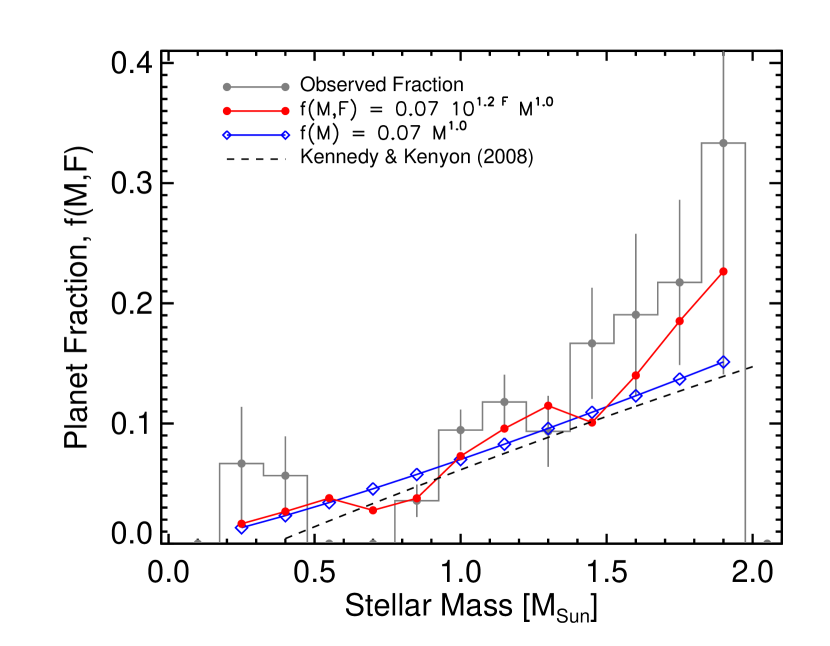
Figure 4.— Planet fraction ($f=N_{planets}/N_{stars}$) as a function of mass for our stellar sample (gray histogram). The red filled circles show the planet fraction predicted by Equation 1 for the masses and metallicities of the stars in each histogram bin. Note that we use a histogram only for visualization purposes; the data were fitted directly without binning. The open diamonds show the best-fitting relationship between planet fraction and stellar mass for [Fe/H] $=0$. The dashed line shows the stellar mass relationship predicted by kennedy08 for Solar metallicity.

The agreement for the low-mass bin is not too surprising since we are using the same sample of M dwarfs as used by Johnson et al. The disagreement for the FGK dwarfs is in part due to the different selection criteria for planet detections: we use a velocity amplitude cutoff of $K>20$ m s^-1, compared to the $M_{P}\sin{i}$ $>0.8$ $M_{\rm Jup}$ used by Johnson et al. Because of this, our sample of planet detections includes a larger number of low-mass planets at short orbital periods, particularly for the Sun-like stellar sample. At higher stellar masses, our measured planet fraction represents a significant refinement over the result of Johnson et al., which stems primarily from our larger sample size and higher Doppler precision with Keck/HIRES compared to Lick/Hamilton.

Our revised planet fraction for the high-mass stars appears much smaller than the recent results presented by bowler10, who measured $f=26^{+9}_{-8}$% for $1.5\leq M_{\star}/M_{\odot}<1.9$, based on the Lick subgiants sample. However, Bowler et al. reported the bulk occurrence rate, and did not attempt to correct or fit for metallicity. Our analysis shows that metallicity plays an important role in shaping the bulk occurrence rate among our subgiants, which are metal-rich by $+0.14$ dex compared to the less massive stars. This can be seen in the highest mass bin in Figure 4, in which the measured planet fraction is consistent with the value measured by Bowler et al. Similarly, in their analysis of the planet fraction for M dwarfs (johnson10a) noted the higher occurrence for metal-rich M dwarfs, but only reported a bulk occurrence rate for the sample.

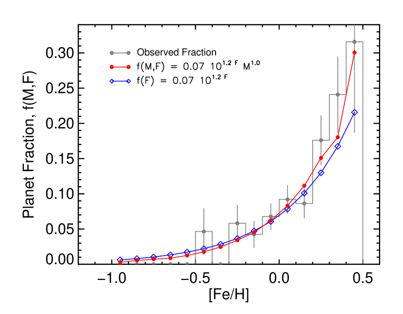
Figure 5.— Planet fraction ($f=N_{planets}/N_{stars}$) as a function of metallicity for our stellar sample (gray histogram). The red filled circles show the planet fraction predicted by Equation 1 for the masses and metallicities of the stars in each bin. Note that we use a histogram only for visualization purposes; the data were fitted directly without binning. The blue open diamonds show the best-fitting relationship between planet fraction and stellar metallicity for $M_{\star}=1$ M_⊙. None of the 52 stars with [Fe/H] $<-0.5$ harbor a giant planet.

6.3. Is there a planet-metallicity correlation among our evolved stars?

In their analysis of the metallicity distribution of K giants with planets, pasquini07 concluded there was no evidence of a PMC among their evolved stars. takeda08 found a similar result based on their sample of massive K giants, while hekker07 did find evidence supporting a PMC among their stellar sample. This somewhat contentious point has important implications for the interpretation of the PMC seen among Sun-like stars. Pasquini et al. argued that this lack of a metallicity correlation was evidence for the “pollution” scenario, in which only the outer layers of stars with planets were metal-enriched by the infall of gas-depleted planetesimals during the planet-formation epoch (gonzalez97; murray02). In this scenario, as stars evolve off of the main sequence their convective envelopes deepen and their polluted outer layers are diluted, erasing any “skin-deep” metallicity enhancement (laughlin00).

In our analysis, we implicitly assume that the PMC holds among the evolved stars in our sample. We can test this assumption by restricting our analysis to $M_{\star}>1.4$ M_⊙ and comparing the Bayesian evidence between two models: planet fraction as a function of stellar mass alone, $f(M)=CM^{\alpha}$ (corresponding to a flat metallicity distribution) versus planet fraction as a function of stellar mass and metallicity, $f(M,F)$, given by Equation 1. We fitted both models to the subsample of massive subgiants, which have deep convective envelopes according to the Padova stellar model grids (girardi02). We find that the planet fraction among these evolved stars is best described as a function of mass and metallicity, with an evidence ratio of order $10^{12}$.

The extreme magnitude of the Bayes factor is driven primarily by the 7 subgiants with $M_{\star}>1.4$ M_⊙ and [Fe/H] $>+0.35$ (Figure 2). It is highly improbable that a flat metallicity distribution would result in 5 out of 7 of these metal-rich subgiants harboring a planet. The best fitting parameters are $\alpha=1.5\pm 0.4$ and $\beta=0.73\pm 0.35$, which are lower than, yet consistent with the values we measure for the full stellar sample. However, the size and metallicity range of our sample of subgiants only allows us to rule out a flat metallicity relationship with 98% confidence. At present we can say that our data are consistent with a PMC among our massive subgiants.

We are not certain about the source of disagreement between our result and those of Pasquini et al. and Takeda et al. One possibility is the difference in our statistical methodologies. Both of those previous studies compared the histograms of stars with and without planets, and as a result did not quantify their confidence in a PMC or lack thereof. It will be informative to apply the techniques outlined in § 4 to the stellar and planet samples of the various K-giant surveys in order to make a meaningful comparison with our results.

7. Summary and Discussion

We have used a large sample of planet-search target stars and planet detections from the CPS to study the correlation between stellar properties and the occurrence of giant planets ($K>20$ m s^-1) with $a\lesssim$2.5 AU. We have derived an empirical relationship describing giant planet occurrence as a function of stellar mass and metallicity, given by

$$f(M_{\star},{\rm[Fe/H]}) = 0.07\pm 0.01\times(M_{\star}/M_{\odot})^{1.0\pm 0.3}$$ (8)

$$\times 10^{1.2\pm 0.2\rm[Fe/H]}.$$

Our understanding of planet formation is presently dominated by two theories: core accretion (e.g. pollack96) and disk instability (boss97). The core accretion model is a bottom-up process, by which protoplanetary cores are built up by the collisions of smaller planetesimals. Once the core reaches a critical mass of roughly 10 $M_{\oplus}$, it rapidly accretes gas from the surrounding disk material. The disk instability mechanism is a top-down process whereby giant planets form from the gravitational collapse of an unstable portion of the protoplanetary disk.

Both models depend on the existence of a massive gas disk, a portion of which forms the bulk of the final mass of the Jupiter-like planet. However, since the inner gas disks of protoplanetary disks disperse on timescales of 3-5 Myr, the process of planet formation is a race against time (e.g. pickett04). In this race the disk instability model holds a major advantage over the core accretion model because, under the right conditions, planets can form from disk collapse in a mere thousands of years, compared to of order Myr timescales required for core accretion.

The disk instability model predicts that there should be no dependence on planet formation and physical stellar properties. The simulations of boss06 showed that giant planets should readily form in even low-mass protoplanetary disks, and that in general giant planets should form efficiently via disk instability independent of stellar mass. The disk instability model also predicts that planet formation should also be independent of disk metallicity (boss02). Indeed, cai06 and meru10 show that the efficiency of disk instability to form giant planets decreases with increasing metallicity.

In contrast to these predictions of the disk instability model, we observe a strong dependence between planet occurrence and the physical properties of the star. Assuming that the present-day mass and metallicity of a star reflects the conditions in its protoplanetary disk, then our results suggest that disk instability is not the primary formation mechanism for the giant planets detected by Doppler surveys. Indeed, it has long been recognized in that there are theoretical complications in forming close-in planets via disk instability boley09. However, the mechanism may be responsible for planets in wide orbits (dr09), however see kratter10 for complications with this scenario.

An alternative explanation for the observed planet-metallicity correlation is the so-called “pollution” model. In this scenario, planet formation actually occurs around stars of all metallicities, and the accretion of gas-depleted protoplanets onto the thin convective layers of stars gives rise to an enhanced stellar metallicity that is actually only ”skin deep” (murray02). pasquini07 interpreted the flat metallicity distribution of K giants with planets as evidence for such an effect, since the deepening convective envelopes of evolved stars should dilute any metallicity enhancement of its outer layers. However, we find that the planet fraction among our massive subgiants is described well by a model with a monotonic rise as a function of both mass and metallicity (Section 6).

While much attention has been given to evolved, intermediate-mass stars in the investigation of the pollution paradigm (laughlin97, FV05), stars at the other end of the stellar mass scale provide another proving ground. M dwarfs have deep convective envelopes over their entire lifetimes, and stars with masses below 0.4 M_⊙ are expected to be completely convective, at least in the absence of strong magnetic activity (e.g. mullan01).

The evidence for a PMC among the subgiants, together with a strong PMC seen among the M dwarfs, are highly suggestive that the present-day metallicities of stars are representative of the compositions of their disks during the planet-formation era. One compelling explanation for both the observed PMC and stellar-mass correlation is that the surface density of solids is a key factor in the planet formation process (laughlin04; ida04; robinson06). If so, both higher stellar (disk) metallicity and higher stellar (disk) mass can generate the requisite surface density for planet formation.

The relationship between planet formation efficiency and stellar mass/metallicity has been previously studied in the context the core accretion paradigm (ikoma00; kornet05; kornet06; kennedy08; thommes08; kretke09; johansen09; mordasini09; dr09). kennedy08 modeled the evolution of the temperature profile at the disk midplanes of stars of various masses, and studied the width of the radial region of disks in which protoplanetary cores form most efficiently. They found that the disks around A-type stars on their descent to the main sequence have very broad formation regions, and their models predicted a positive correlation between stellar mass and giant planet formation efficiency. Their prediction for the planet fraction is shown as a dashed line in Figure 4, which we have approximated using the polynomial relationship $f(M)=-0.03633+0.0138M_{\star}-0.0060M_{\star}^{2}$. The agreement between theory and observation is striking.

The interplay between the mass and metallicity of protoplanetary disks is also apparent in the core accretion simulations of thommes08. In their analysis, they simulated disks with a wide variety of masses, viscosities and metallicities. Their models produce gas giants most effectively in disks with a combination of high masses ($M_{\rm disk}\gtrsim 0.04$ M_⊙) and low viscosities. In their simulations of the effects of metallicity, they found that gas giants can form in Solar-composition disks only if the disk masses exceed $\approx 0.06$ M_⊙, or twice the minimum-mass Solar nebula. This mass threshold decreases to $\approx 0.03$ M_⊙ for disks with [Fe/H] $=0.25$. Thus, Thommes et al. showed that there can be a trade-off between the mass and metallicity of a protoplanetary disk in forming giant planets. In the core accretion paradigm, M dwarfs can form giant planets, but only if they have high metallicities. Similarly, even low-metallicity A stars can form massive planets, owing to their more massive disks (see also dr09).

Theories of planet formation have progressed in large leaps thanks largely to the rapidly growing sample of exoplanets discovered around other stars. Successful, generalized theories of the origins of planetary systems must account for the observed correlations between planet occurrence and stellar properties. The findings presented herein are the result of more than 15 years of high-precision Doppler monitoring of nearby stars. Additional information will soon pour in from other surveys using techniques such as microlensing (e.g. dong09; gould10), astrometry (boss09), transits (kepler; corot1; irwin09) and direct imaging (sphere; nici; gpi).

Our results have important implications for the target selection of these future planet surveys. We find that A-type stars harbor planets at an elevated rate compared to less massive stars. However, it is not obvious whether A type stars make the most promising targets for other types of surveys. Where massive stars perhaps hold the most promise is for direct imaging surveys. The first two planetary systems imaged around normal stars were both young A-type dwarfs (kalas08; marois08). Are A dwarfs the ideal direct imaging targets? The answer to this question will rely on the results presented herein, along with a careful consideration of the mass, metallicity, luminosity and age distributions of nearby stars; and the orbital and physical properties of planets as a function of stellar mass. This issue will be addressed in a companion paper (Crepp & Johnson 2010).