Nematic liquid crystal dynamics under applied electric fields

Abstract

In this paper we investigate the dynamics of liquid crystal textures in a two-dimensional nematic under applied electric fields, using numerical simulations performed using a publicly available LIquid CRystal Algorithm (LICRA) developed by the authors. We consider both positive and negative dielectric anisotropies and two different possibilities for the orientation of the electric field (parallel and perpendicular to the two-dimensional lattice). We determine the effect of an applied electric field pulse on the evolution of the characteristic length scale and other properties of the liquid crystal texture network. In particular, we show that different types of defects are produced after the electric field is switched on, depending on the orientation of the electric field and the sign of the dielectric anisotropy.

I Introduction

Defects in the nematic liquid crystalline phase may appear when the symmetry of the isotropic phase is broken in a isotropic-nematic phase transition, or as a topological response to imposed boundary conditions de Gennes and Prost (1995). Confined nematics is a stimulating field of recent research Shin et al. (2008); Xing (2008); Lopez-Leon and Fernandez-Nieves (2009); Kamien et al. (2009) due to the possibility of different technological applications. The similarity with defect formation in the early universe has also turned liquid crystals into mini laboratories for testing the formation and dynamics of cosmic topological defects Chuang et al. (1991); Digal et al. (1999); Avelino et al. (2006); Mukai et al. (2007); Avelino et al. (2008). It has also led one of us (FM) and co-workers to explore the optical properties of defects in a liquid crystal in a geometric setting very much like their cosmic analogues Sátiro and Moraes (2005, 2006); Carvalho et al. (2007); Sátiro and Moraes (2008).

The complexity of the (dis)organization of nematic molecules in the presence of defects limits severely what can be analysed using analytical tools. Hence, computer simulations are an important complement in the study of the evolution of liquid crystalline systems with defects. Lattice simulations have been used extensively in the study of liquid crystals (see, for example, Billeter et al. (1999); Priezjev and Pelcovits (2002); Slavin et al. (2006); Bhattacharjee et al. (2008); de las Heras et al. (2009)) since the pioneering work of Lebwohl and Lasher Lebwohl and Lasher (1972). An order parameter is usually attached to each point of the lattice with orientational degrees of freedom only, so that the liquid does not flow but each molecule is free to orient itself in three-dimensional space. The fact that a relatively large number of particles enter the simulation is particularly useful to study collective behavior such as phase transitions and systems presenting large scale fluctuations and defects.

From the industry point of view, defects may be quite relevant. They are a problem for liquid crystal displays since they scatter light, but they are unavoidable in the switching of the cells. Consequently, it is interesting, both from scientific and technological points of view, to study how applied external electric fields influence the formation and dynamics of defects in nematics. External electric or magnetic fields couple to the director adding an extra ingredient to an already complex problem Dierking et al. (2005); Fukuda et al. (2009); Gartland et al. (2010); Singh et al. (2010); Prakash et al. (2005); Ostapenko et al. (2008); Fukuda (2010).

In this work we simulate the dynamics of defects in a two-dimensional nematic in the presence of an applied electric field, after quenching from the isotropic phase. The outline of this paper is as follows. In Sec. II we present the Landau-de Genes theory which we use to model the relaxational dynamics of nematic liquid crystals under applied electric fields. In Sec. III we report on a publicly available LIquid CRystal Algorithm (LICRA) developed by the authors and describe the specific numerical implementation used in this paper. In Sec. IV the results are presented, considering different possibilities for the orientation of the electric field and sign of the dielectric anisotropy. We conclude in Sec. V.

II Landau-de Gennes theory

The orientational order of a nematic liquid crystal is described by a symmetric traceless tensor, ${\bf Q}$, whose components are given by de Gennes and Prost (1995).

$$Q_{\alpha\beta}({\bf r}) = -\frac{1}{3}\delta_{\alpha\beta}+\langle{u_{\alpha}u_{\beta}}\rangle$$ (1)

$$= -\frac{1}{3}\delta_{\alpha\beta}+\int d^{2}{\bf u}\,f({\bf r},{\bf u},t)u_{\alpha}u_{\beta}\,,$$

where $f({\bf r},{\bf u},t)$ is the the molecular orientational distribution function at the position ${\bf r}$ and time $t$, measuring the number of molecules with orientation defined by the unit vector ${\bf u}$ with components $u_{\alpha}$. The order parameter, ${\bf Q}$, can be written as a function of the principal values $S$ and $T$ and the eigenvectors ${\bf n}$ (the director), ${\bf l}$ (the codirector) and ${\bf m}={\bf n}\times{\bf l}$. Its components are given by

$$Q_{\alpha\beta}=\frac{3}{2}S\mbox{$\hskip 1.00006pt\stackrel{{\scriptstyle\rule{0.4pt}{0.8288pt}\hskip 2.79996pt\!\!\!\overline{\hskip 0.41998pt\vphantom{\rule{0.4pt}{0.0pt}}\hphantom{\mbox{$\displaystyle n_{\alpha}n_{\beta}$}}\hskip 0.41998pt}\!\!\!\hskip 2.79996pt\rule{0.4pt}{0.8288pt}}}{{n_{\alpha}n_{\beta}}}\hskip 1.99997pt$ }-\frac{1}{2}T\left(l_{\alpha}l_{\beta}-m_{\alpha}m_{\beta}\right)\,,$$ (2)

where

$$\mbox{$\hskip 1.00006pt\stackrel{{\scriptstyle\rule{0.4pt}{0.8288pt}\hskip 2.79996pt\!\!\!\overline{\hskip 0.41998pt\vphantom{\rule{0.4pt}{0.0pt}}\hphantom{\mbox{$\displaystyle X_{\alpha\beta}$}}\hskip 0.41998pt}\!\!\!\hskip 2.79996pt\rule{0.4pt}{0.8288pt}}}{{X_{\alpha\beta}}}\hskip 1.99997pt$ }=\frac{1}{2}\left(X_{\alpha\beta}+X_{\beta\alpha}\right)-\frac{1}{3}\delta_{\alpha\beta}X_{\gamma\gamma}\,.$$ (3)

Defining $\theta$ and $\phi$ such that $\cos\theta={\bf u}\cdot{\bf n}$, $\sin\theta\cos\phi={\bf u}\cdot{\bf l}$ and $\sin\theta\sin\phi={\bf u}\cdot{\bf m}$, the principal values $S$ and $T$ can be written as

$$S = \langle\cos^{2}\theta\rangle-\frac{1}{3}\,,$$ (4)

$$T = \langle{\sin^{2}\theta\cos 2\phi}\rangle\,.$$ (5)

The inner product is defined by ${\bf a}\cdot{\bf b}=a_{\gamma}b_{\gamma}$ where we use the Einstein notation for the summation of repeated indices. Also, note that in Eq. (1) $d^{2}{\bf u}=\sin^{2}\theta\,d\theta\,d\phi$.

The free energy is given by

$$F=\int d^{3}{\bf r}\left(\mathcal{F}_{I}+\mathcal{F}_{II}+\mathcal{F}_{III}\right)\,,$$ (6)

where $\mathcal{F}_{I}$ is obtained from a local expansion in powers of rotationally invariant powers of the order parameter

$$\mathcal{F}_{I}=\frac{A}{2}\,Q_{2}+\frac{B}{3}\,Q_{3}+\frac{C}{4}\,Q_{2}^{2}+\frac{D}{6}\,Q_{3}^{2}\,,$$ (7)

$\mathcal{F}_{II}$ is a non-local contribution arising from rotationally invariant combinations of gradients of the order parameter

$$\mathcal{F}_{II}=\frac{R_{1}}{2}\,\partial_{\alpha}Q_{\beta\gamma}\,\partial_{\alpha}Q_{\beta\gamma}+\frac{R_{2}}{2}\,\partial_{\alpha}Q_{\alpha\beta}\,\partial_{\gamma}Q_{\beta\gamma}\,,$$ (8)

and $\mathcal{F}_{III}$ accounts for the effect of an external electric field ${\bf E}$

$$\mathcal{F}_{III}=-\frac{\tau_{E}}{2}Q_{\alpha\beta}E_{\alpha}E_{\beta}\,,$$ (9)

where $\tau_{E}=2\Delta\epsilon$ and $\Delta\epsilon$ is the dielectric anisotropy.

Static equilibrium can only be reached for a minimum value of the free energy ($\delta F/\delta Q_{\mu\nu}=0$). However, the evolution of the order parameter $\bf Q$ from a given set of initial conditions is not fully specified by the free energy functionals, and further assumptions have to be made on how the minimization process will take place. In the absence of thermal fluctuations and hydrodynamics flow, the time evolution of the order parameter is given by

$${\dot{Q}}_{\alpha\beta}({\bf r},t)=-\Gamma_{\alpha\beta\mu\nu}\frac{\delta F}{\delta Q_{\mu\nu}}\,.$$ (10)

Here the dot represents derivative with respect to the physical time, $t$, and the tensor

$$\Gamma_{\alpha\beta\mu\nu}=\Gamma\left(\delta_{\alpha\mu}\delta_{\beta\nu}+\delta_{\alpha\nu}\delta_{\beta\mu}-\frac{2}{3}\delta_{\alpha\beta}\delta_{\mu\nu}\right)\,,$$ (11)

satisfies $\Gamma_{\alpha\beta\mu\nu}=\Gamma_{\beta\alpha\mu\nu}=\Gamma_{\mu\nu\alpha\beta}$ and $\Gamma_{\alpha\alpha\mu\nu}=0$ thus ensuring that the order parameter $\bf Q$ remains symmetric and traceless. In the following we shall assume that the kinetic coefficient, $\Gamma$, is a constant.

The equation of motion can be written more explicitly as

$${\dot{Q}}_{\alpha\beta} = -\Gamma[(A+CQ_{2})Q_{\alpha\beta}+(B+DQ_{3})\mbox{$\hskip 1.00006pt\stackrel{{\scriptstyle\rule{0.4pt}{0.8288pt}\hskip 2.79996pt\!\!\!\overline{\hskip 0.41998pt\vphantom{\rule{0.4pt}{0.0pt}}\hphantom{\mbox{$\displaystyle Q_{\alpha\gamma}Q_{\gamma\beta}$}}\hskip 0.41998pt}\!\!\!\hskip 2.79996pt\rule{0.4pt}{0.8288pt}}}{{Q_{\alpha\gamma}Q_{\gamma\beta}}}\hskip 1.99997pt$ }$$ (12)

$$-R_{1}Q_{\alpha\beta,\gamma\gamma}-R_{2}\mbox{$\hskip 1.00006pt\stackrel{{\scriptstyle\rule{0.4pt}{0.8288pt}\hskip 2.79996pt\!\!\!\overline{\hskip 0.41998pt\vphantom{\rule{0.4pt}{0.0pt}}\hphantom{\mbox{$\displaystyle Q_{\beta\gamma,\gamma\alpha}$}}\hskip 0.41998pt}\!\!\!\hskip 2.79996pt\rule{0.4pt}{0.8288pt}}}{{Q_{\beta\gamma,\gamma\alpha}}}\hskip 1.99997pt$ }-\tau_{E}\mbox{$\hskip 1.00006pt\stackrel{{\scriptstyle\rule{0.4pt}{0.8288pt}\hskip 2.79996pt\!\!\!\overline{\hskip 0.41998pt\vphantom{\rule{0.4pt}{0.0pt}}\hphantom{\mbox{$\displaystyle E_{\alpha}E_{\beta}$}}\hskip 0.41998pt}\!\!\!\hskip 2.79996pt\rule{0.4pt}{0.8288pt}}}{{E_{\alpha}E_{\beta}}}\hskip 1.99997pt$ }]\,,$$

where a comma denotes a partial derivative.

III Numerical implementation

We solve Eq. (12) using a standard second-order finite difference algorithm for the spatial derivatives and a second order Runge-Kutta method for the time integration. All the simulations are performed on a two dimensional $256^{2}$ grid (in the $xy$ plane) with periodic boundary conditions. The order parameter ${\bf Q}$ has 5 degrees of freedom associated with $S$, $T$, $\bf n$, $\bf l$ ($\bf n$ accounts for two degrees of freedom). In the simulations, the initial conditions for $S$ and $T$ are randomly generated, at every grid point, from uniform distributions in the intervals $[0,1[$ and $[0,S[$, respectively. The director, ${\bf n}$, is also randomly generated, at every grid point, using the spherical vector distribuitions routines in the GNU Scientific Library and the codirector, $\bf l$ , was calculated by randomly choosing a direction perpendicular to ${\bf n}$.

We start our simulations with the electric field switched off, switching it on at a given time, $t_{\rm on}=400$, and disconnecting it at a later time, $t_{\rm off}=600$. We consider two different possibilities for the orientation of the applied electric field, perpendicular or parallel to the plane of the simulation. In each case we consider situations with either positive ($\Delta\epsilon>0$) or negative ($\Delta\epsilon<0$) dielectric anisotropies. The parameters used in the simulations are $\Delta x=\Delta y=1$, $\Delta t=0.1$ and $A=-0.1$, $B=-0.5$, $C=2.67$, $R_{1}=1.0$, $R_{2}=0.0$, $\Gamma=1.0$, corresponding to a uniaxial nematic phase Bhattacharjee et al. (2008)). The amplitude of the applied rectangular electric field pulse is taken to be $E=0.025/{\sqrt{|\Delta\epsilon|}}$.

In order to determine the evolution of the characteristic scale of the network we numerically calculate the function

$$P({\bf k},t)=\frac{Q_{\alpha\beta}({\bf k},t)Q_{\beta\alpha}({\bf-k},t)}{\int{d^{3}{\bf k}\;Q_{\alpha\beta}({\bf k},t)Q_{\beta\alpha}({\bf-k},t)}}\,,$$ (13)

after setting the infinite wavelength mode $Q_{\alpha\beta}({\bf 0})$ to zero. Here $Q_{\alpha\beta}({\bf k})$ is the Fourier transform of $Q_{\alpha\beta}({\bf r})$ (${\bf k}$ is the wavenumber). The characteristic scale, $L$, can then be defined as

$$\frac{1}{L^{2}}=\langle k^{2}\rangle=\sum_{{\bf k}}k^{2}P({\bf k},t)/\sum_{\bf k}P({\bf k},t)\,.$$ (14)

The set of C codes used to perform the simulation are available at http://faraday.fc.up.pt/licra along with Matlab/Octave routines that are used to generate the results visualization. This software is free and we have named it LICRA (LIquid CRystal Algorithm). LICRA can be used to perform numerical simulation of the dynamics of liquid crystal texture networks in both two- and three-dimensional nematics. LICRA also accounts for the application of an external electric field on the system. Simulation parameters may be modified in the file licra.h or directly on the code which is properly commented for this effect. The GNU Compiler Collection (gcc) and both the Fastest Fourier Transform in the West (FFTW) and the GNU Scientific Library (GSL) are required in order to compile the source code.

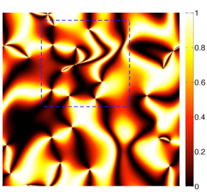
(a)

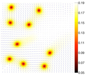
(b)

(c)

Figure 1: Topological defects in a coarsening nematic liquid crystal before the application of an external electric field. Fig. 1a represents the value of $\sin^{2}(2\chi)$ at every grid point (note that both half-integer and integer disclinations appear in the simulations). Fig. 1b shows the value of the parameter $S$ at every grid point inside the dashed region, as well as the projection of the director ${\bf n}$ onto the two dimensional grid. In Fig. 1c the value of the parameter $T$ in same region is given.

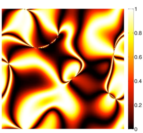
Figure 2: Similar to Fig. 1a but now after the application of an electric field pulse perpendicular to the lattice plane. The figure shows that, in the case of a positive dielectric anisotropy ($\Delta\epsilon>0$), only integer ($\pm 1$) disclinations remain in the simulation, after the application of the external electric field.

The code outputs contain the results for the order parameter $S$ and $T$, the director and codirector components at each grid point and the angle between the projection of the director onto the $x-y$ plane and the $x$ axis. The visualization routines generate the intensity of the transmitted light after passing thought a nematic liquid crystal sample with crossed polarizers, the parameters $S$ and $T$, and the evolution of characteristic length scale with time.

IV Results

Fig. 1 represents a texture network in a coarsening nematic liquid crystal just before the application of an external electric field at $t=t_{\rm on}$. The value of $\sin^{2}(2\chi)$ is plotted in Fig. 1a, where $\chi$ is the angle of an arbitrary axis on the plane of the simulation with the projection of the director ${\bf n}$ onto the same plane. Topological defects of both half-integer ($\pm 1/2$) and integer ($\pm 1$) charge appear in the simulations, corresponding to the meeting points of two and four dark brushes, respectively. Schlieren patterns similar to the ones shown in Fig. (1a) may be obtained experimentally using a linear polarized light microscope with a liquid crystal sample placed between crossed polarizers.

Fig. 1b shows the value of $S$ at every grid point inside the dashed region as well as the projection, onto the two dimensional grid, of the director ${\bf n}$. In Fig. 1c the value of the parameter $T$ is also shown for the same region. There is a rapid variation of the parameters $S$ and $T$ at the half-integer charge defect cores while no significant variation occurs in the case of integer charge defects. The non-zero values of $T$ are due to the biaxiality inside half-integer defect cores Schopohl and Sluckin (1987). It is also clear that integer charge defects are associated with regions where the projection of the director ${\bf n}$, onto the two-dimensional grid, is very small.

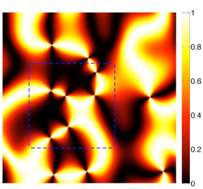
(a)

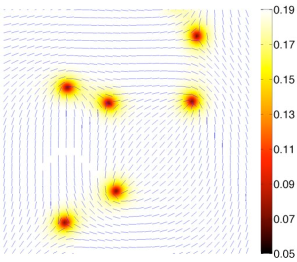
(b)

Figure 3: Similar to Figs. 1a and 1b except that now a negative dielectric anisotropy ($\Delta\epsilon<0$) was considered (again with an electric field pulse perpendicular to the lattice plane). In this case, only half-integer ($\pm 1/2$) disclinations survive, after the application of the external electric field.

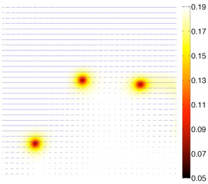
Figure 4: The figure represents the order parameter $S$ as well as the projection of the director, ${\bf n}$, onto the two-dimensional grid, after the application of an electric field pulse parallel to the lattice plane. A negative dielectric anisotropy ($\Delta\epsilon<0$) was considered in this case. All the defects appearing in the simulations correspond to half-integer twisted disclinations.

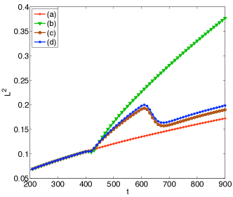
Figure 5: The evolution of the correlation length, $L(t)$, in four different situations: $(a)$ without external electric field, $(b)$ with an electric field perpendicular to the lattice plane and $\Delta\epsilon>0$, $(c)$ the same as $(b)$ but with $\Delta\epsilon<0$ and $(d)$ with an electric field parallel to the lattice plane and $\Delta\epsilon<0$. The electric field is connected when $t=t_{\rm on}=400$ and disconnected when $t=t_{\rm off}=600$.

Figs. 2, 3 and 4 represent a texture network in a coarsening nematic liquid crystal after the application of an external electric field ($t=800\ (>t_{\rm off})$). Fig. 3 shows the value of $\sin^{2}(2\chi)$ at every grid point after the application of an electric field pulse perpendicular to the lattice in the case of a positive dielectric anisotropy ($\Delta\epsilon>0$). After the field is switched on, the molecules (and the director ${\bf n}$ at each grid point) tend to become aligned parallel to the field, which results in the rapid suppression of half-integer disclinations (only integer ones remain in the simulations). Accordingly, $S$ is roughly constant and $T$ is very close to zero at all network points. In this case the projection of the director ${\bf n}$, onto the two-dimensional grid, is very small at every grid point. Apart from the modification of the background values of $S$ and $T$ there is no significant modification to the network evolution when the electric field is switched off (this can be confirmed in Fig. 5).

(a)

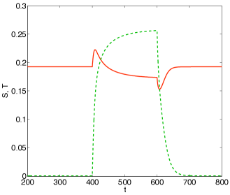
(b)

Figure 6: Figs. 6a and 6b represent the evolution of the parameters $S$ and $T$ for the case of an homogeneous director, ${\bf n}$, initially aligned parallel to the lattice plane considering, respectively, either a positive ($\Delta\epsilon>0$) or negative ($\Delta\epsilon<0$) dielectric anisotropy. In both cases an electric field perpendicular to the plane is connected for $t=t_{\rm on}=400$ and disconnected for $t=t_{\rm off}=600$.

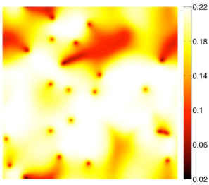
(a)

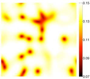
(b)

Figure 7: Figs. 7a and 7b represent the order parameter $S$ at every grid point at the times corresponding to the maximum and minimum of $S$ in Fig. 6b, after the application of an electric field perpendicular to the lattice plane, for a negative dielectric anisotropy ($\Delta\epsilon<0$).

Figs. 3a and 3b are analogous to Figs. 1a and 1b except that, in this case, a negative dielectric anisotropy ($\Delta\epsilon<0$) was considered (again with an electric field pulse perpendicular to the lattice plane). After the electric field is switched on the molecules (and the director ${\bf n}$) tend to become perpendicular to the electric field, which results in the rapid suppression of integer disclinations (only half-integer ones remain in the simulations). As expected there is a rapid variation of the parameter $S$ (and $T$) at the half-integer charge defect cores, which can be seen in Fig. 3b.

If the electric field is applied in a direction parallel to the plane of the simulation and $\Delta\epsilon>0$ then the director ${\bf n}$ at each grid point will become aligned parallel to the electric field and both integer and half-integer defects are suppressed. The most interesting situation, with the electric field parallel to the lattice plane, is that of a negative dielectric anisotropy ($\Delta\epsilon<0$). In this case, the director ${\bf n}$ at each grid point becomes perpendicular to the electric field generating half-integer twist disclinations Billeter et al. (1999); Callan-Jones et al. (2006). The value of $\sin^{2}(2\chi)$ is equal to zero at every grid point but the defects can be seen in Fig. 4 which shows the order parameter $S$ at various grid points as well as the projection of the director ${\bf n}$ onto the lattice plane. All the defects appearing in the simulations correspond to half-integer twisted disclinations which can be identified by the values of the projections of ${\bf n}$ around them.

The evolution of the characteristic length scale, $L(t)$, is shown in Fig. 5, in units of the simulation box size. Four different situations have been considered: $(a)$ without external electric field, $(b)$ with an electric field perpendicular to the lattice plane and $\Delta\epsilon>0$, $(c)$ the same as $(b)$ but with $\Delta\epsilon<0$ and $(d)$ with an electric field parallel to the lattice plane and $\Delta\epsilon<0$. In each case an average over $100$ different simulations with random initial conditions considering has been made. The electric field is connected at the time $t=t_{\rm on}=400$ and disconnected at $t=t_{\rm off}=600$. In all cases the characteristic length scale evolves roughly as $L^{2}\propto t$ but the slope is rapidly modified when the electric field is switched on (or switched off in cases (c) and (d)).

Figs. 6a and 6b show the evolution of the parameters $S$ and $T$ for the case of an homogeneous director, ${\bf n}$, initially aligned parallel to the lattice plane considering, respectively, either a positive ($\Delta\epsilon>0$) or negative ($\Delta\epsilon<0$) dielectric anisotropy. In both cases an electric field perpendicular to the plane is connected for $t=t_{\rm on}=400$ and disconnected for $t=t_{\rm off}=600$. As expected, Fig. 6a shows that the system develops a large biaxiality right after the electric field is switched on since, initially, there are two distinct preferred directions defined by the director and the external electric field. After some time, the director becomes aligned with the electric field ($\Delta\epsilon>0$), $T$ is again driven towards zero and $S$ tends to larger value than before the electric field is switched on (this is expected since the dispersion of molecular orientations around ${\bf n}$, is reduced due to the external electric field). After the electric field is switched off at $t=t_{\rm off}$, $S$ returns to the value it had before $t_{\rm on}$.

For $\Delta\epsilon<0$, Fig. 6b shows that again the system develops a large biaxiality right after the electric field is generated but, in this case, the biaxiality does not go away before $t_{\rm off}$ since the two distinct preferred directions defined by the director and the external electric field will remain perpendicular to each other. Right after the electric field is switched on, the value of $S$ increases sharply, before moving to a value smaller than before $t_{\rm on}$. The sharp growth of $S$ right after $t_{\rm on}$ is due to an initial decrease of the dispersion of molecular orientations around ${\bf n}$ due to the presence of the external electric field. In the subsequent evolution of $S$, before $t_{\rm off}$, the molecules are forced into the plane by the perpendicular electric field. This accounts for the fact that the value of $S(t_{\rm on})$ is slightly smaller than $S(t_{\rm off})$. Right after $t_{\rm off}$ the value of $T$ decreases sharply towards zero, which is responsible for corresponding sharp decrease of $S$. After that, $S$ increases again returning to the value it had before $t_{\rm on}$.

Figs. 7a and 7b represent the parameter, $S$, at every grid point, at the times corresponding to the maximum and minimum of $S$ in Fig. 6b, after the application of an electric field pulse perpendicular to the lattice plane, for a negative dielectric anisotropy ($\Delta\epsilon<0$). They confirm the background evolution shown in Fig. 6b and they also reveal a dramatic change on the characteristic scale of defect cores which is associated with the behaviour of the characteristic scale shown in Fig. 5 for cases (c) and (d).

V Conclusions

In this paper we investigated the effect that an applied electric field pulse has on the dynamics of a liquid crystal texture network, using numerical simulations performed with LICRA, a publicly available LIquid CRystal Algorithm developed by the authors. We have demonstrated that the presence of an electric field can lead to significant changes of the molecular orientational distribution function, including the background value of the parameters $S$ ad $T$ as well as their profile at the defect cores. We have further shown that an electric field pulse may lead to a defect network whose properties depend on the orientation of the applied electric field and the sign of the dielectric anisotropy. Depending on the case, topological defects with integer or half integer topological charges remain after the electric pulse has been applied. In summary, our results describe how an applied electric field can be used to as control the nature of the defects in a liquid crystal texture network.