Confinement-induced resonance in quasi-one-dimensional systems under transversely anisotropic confinement

Abstract

We theoretically investigate the confinement-induced resonance for quasi-one-dimensional quantum systems under transversely anisotropic confinement, using a two-body s-wave scattering model in the zero-energy collision limit. We predict a single resonance for any transverse anisotropy, whose position shows a slight downshift with increasing anisotropy. We compare our prediction with the recent experimental result by Haller et al. [Phys. Rev. Lett. 104, 153203 (2010)], in which two resonances are observed in the presence of transverse anisotropy. The discrepancy between theory and experiment remains to be resolved.

I Introduction

Recently ultracold low-dimensional atomic gases have attracted a great deal of interest as they show unique quantum signatures not encountered in three dimension (3D) LowDimRMP . For example, a one-dimensional (1D) gas of bosonic atoms with strongly repulsive interparticle interactions acquires fermionic properties Petrov . A 1D gas of fermionic atoms may exhibit exotic inhomogeneous superfluidity hldprl2007 ; xiajifflo2007 ; xiajifflo2008 and cluster-pairing xiajiclusterpairing . In two dimensions, the Berezinskii-Kosterlitz-Thouless (BKT) phase transition is very different from the usual finite-temperature phase transitions Dalibard . Experimentally, ultracold low-dimensional atomic systems are conveniently accessible upon introducing tight confinement via optical lattices that remove one or two spatial degrees of freedom LowDimRMP . Furthermore, the interactions between atoms can also be tuned precisely and arbitrarily by a collisional Feshbach resonance Feshbach1962 ; FRreview . Using these means, low-dimensional atomic systems now provide an ideal experimental model to test fundamental many-body physics, and are much simpler than corresponding systems in condensed matter physics.

Confinement-induced resonance (CIR) is an intriguing phenomenon found when one relates the effective 1D coupling constant of quasi-1D quantum gases, $g_{1D}$, to the 3D s-wave scattering length, $a_{3D}$ Olshanii1998 ; Bergeman2003 ; Kim2005 ; Mora ; Naidon2007 ; Saeidian . Considering a tight transverse confinement ($\omega_{\perp}=\omega_{x}=\omega_{y}$) with the characteristic length scale $a_{\perp}=\sqrt{\hbar/(m\omega_{\perp})}$, Olshanii showed that the effective 1D coupling strength diverges at a particular ratio of $a_{3D}/a_{\perp}$ Olshanii1998 . The underlying physics of the CIR is very similar to the well-known Feshbach resonance Bergeman2003 , if we assume that under tight confinement the ground-state transverse mode and the other transverse modes play respectively the roles of the scattering “open” channel and “closed” channels. The scattering state of two colliding atoms in the ground-state transverse mode can be brought into resonance with a bound molecular state in other high-lying transverse modes by tuning the ratio of $a_{3D}/a_{\perp}$. This causes a confinement induced resonance.

This type of novel resonance was recently confirmed in several ultracold atom experiments Kinoshita ; Paredes ; Esslinger ; Haller2009 ; Haller2010 . In particular, the properties of CIR for an ultracold quantum gas of Cs atoms were studied systematically by measuring atom loss and heating rate under transversely anisotropic confinement near a rather narrow Feshbach resonance Haller2010 . Upon increasing the transverse anisotropy, two CIRs were observed, splitting from the single CIR in the isotropic limit.

In this paper, we theoretically investigate the CIR under transversely anisotropic confinement, using a zero-energy pseudopotential approach Olshanii1998 , which is a useful generalization of Olshanii’s method. We find a single resonance in the scattering amplitude, except with a downshift of the resonance position with increasing transverse anisotropy. We calculate also the bound state of the decoupled excited transverse manifold and find only one such bound state exists. Taken together, we believe that there is only one CIR in an anisotropic two-body s-wave scattering model at zero-energy limit. The two (splitting) resonances found experimentally therefore must be caused by some other reasons beyond the simple s-wave, zero-energy scattering model.

In the following, we first present the essence of s-wave scattering approach and calculate the bound state of the excited transverse manifold (Sec. II) and then discuss in detail the CIR as a function of the transverse anisotropy (Sec. III). Sec. IV is devoted to conclusions and further remarks.

II CIR under transversely anisotropic confinement

II.1 The scattering amplitude

In this section, we calculate the effective 1D coupling constant under transversely anisotropic confinement by generalizing the zero-energy s-wave scattering approach developed by Olshanii Olshanii1998 . Let us consider two atoms in a harmonic trap with weak confinement in $z$-axis and tight confinement in the transverse direction such that $\omega_{x}=\eta\omega_{y}\gg\omega_{z}$. The transverse anisotropy is characterized by the ratio $\eta=\omega_{x}/\omega_{y}$ . The motion along the $z$-axis is approximately free. To consider the scattering in this direction, we therefore set $\omega_{z}=0$. Owing to the separability of center-of-mass motion and relative motion in harmonic traps, the low-energy s-scattering along z-axis is described by the following single-channel Hamiltonian:

$$\hat{H}_{rel}=-\frac{\hbar^{2}}{2\mu}\frac{\partial^{2}}{\partial z^{2}}+{\cal\hat{H}}_{\bot}+g_{3D}\delta({\bf r})\frac{\partial}{\partial r}r,$$ (1)

where

$$\hat{H}_{\perp}=-\frac{\hbar^{2}}{2\mu}\left(\frac{\partial^{2}}{\partial x^{2}}+\frac{\partial^{2}}{\partial y^{2}}\right)+\frac{1}{2}\mu\omega_{y}^{2}\left(\eta^{2}x^{2}+y^{2}\right),$$ (2)

Here, $g_{3D}=4\pi\hbar^{2}a_{3D}/m$ is the 3D coupling constant, and $\mu=m/2$ is the reduced mass for the relative motion. The effective 1D coupling constant $g_{1D}$ is obtained by matching the scattering amplitude of the exact 3D solution $\Psi({\bf r})$ of Eq. (1) to that of a 1D Hamiltonian

$${\cal H}_{1D}=-\frac{\hbar^{2}}{2\mu}\frac{\partial^{2}}{\partial z^{2}}+g_{1D}\delta(z).$$ (3)

The latter scattering amplitude $f_{e}(k_{z})$, with low scattering energy $E=\hbar^{2}k_{z}^{2}/2\mu$, is then given by,

$$\Psi(x=0,y=0,z)\propto e^{ik_{z}z}+f_{e}(k_{z})e^{ik_{z}\left|z\right|}$$ (4)

for $\left|z\right|\rightarrow\infty$ , and the effective 1D coupling constant $g_{1D}$ can be determined by using

$$g_{1D}=\lim_{k_{z}\rightarrow 0}\frac{\hbar^{2}k_{z}}{\mu}\frac{\mathop{\rm Re}f_{e}(k_{z})}{\mathop{\rm Im}f_{e}(k_{z})}.$$ (5)

Next, we shall calculate the 3D exact solution $\Psi({\bf r})$, from which we can extract the effective 1D scattering amplitude $f_{e}(k_{z})$ at the collision energy $E=\hbar^{2}k_{z}^{2}/2\mu+\hbar\omega_{x}/2+\hbar\omega_{y}/2$, when $k_{z}\rightarrow 0$. Using the complete set of eigenstates of the non-interacting Hamiltonian, the (un-normalized) scattering wavefunction can be expanded as,

$$\Psi({\bf r})=\int_{-\infty}^{\infty}dk\sum_{n_{1},n_{2}}A_{n_{1}n_{2}}\left(k\right)\phi_{n_{1}}(\frac{\sqrt{\eta}x}{d})\phi_{n_{2}}(\frac{y}{d})e^{ikz},$$ (6)

where $\phi_{n}(\xi)=(\sqrt{\pi}2^{n}n!)^{-1/2}e^{-\xi^{2}/2}H_{n}\left(\xi\right)$ is the $n$-th eigenstate of a 1D harmonic oscillator ($n=0,2,4,...$), and $d=\sqrt{\hbar/\left(\mu\omega_{y}\right)}$ is the oscillator length in the $y$-axis. In the summation, the integers $n_{1},n_{2}$ can be restricted to even numbers, as $s$-wave scattering preserves parity. The expansion coefficients $A_{n_{1}n_{2}}(k)$ may be determined by substituting the wavefunction (6) into the Schrödinger equation $\hat{H}_{rel}\Psi({\bf r})=E\Psi({\bf r})$ and then projecting both sides of the equation onto noninteracting states (i.e., the expansion basis) Busch ; Idziaszek ; Liang . Owing to the contact interaction, the expansion coefficient takes the form,

$$A_{n_{1}n_{2}}(k)=-\frac{g_{3D}\phi_{n_{1}}^{*}(0)\phi_{n_{2}}^{*}(0){\cal F}}{n_{1}\hbar\omega_{x}+n_{2}\hbar\omega_{y}+\frac{\hbar^{2}}{2\mu}\left(k^{2}-k_{z}^{2}\right)},$$ (7)

depending on a single parameter

$${\cal F}=\left[\frac{\partial\left(r\Psi({\bf r})\right)}{\partial r}\right]_{r=0}=\left[\frac{\partial\left(z\Psi(0,0,z)\right)}{\partial z}\right]_{z\rightarrow 0^{+}}.$$ (8)

The summation over $n_{1},n_{2}$ and $k$ in the scattering wavefunction $\Psi({\bf r})$ can then be performed Idziaszek ; Liang , yielding

$$\frac{\Psi\left(0,0,z\right)}{\phi_{0}^{2}\left(0\right)} = e^{ik_{z}z}-i\frac{\eta^{1/4}\mu g_{3D}{\cal F}}{\sqrt{\pi}\hbar^{2}dk_{z}}e^{ik_{z}|z|}$$ (9)

$$-\frac{\eta^{1/4}g_{3D}\mu{\cal F}}{2\sqrt{\pi}\hbar^{2}}\Lambda\left[\frac{2\left|z\right|}{d},-\left(\frac{dk_{z}}{2}\right)^{2}\right],$$

where the function $\Lambda[\xi,\epsilon]$ takes the form

$$\Lambda=\int\limits_{0}^{\infty}dt\frac{e^{-\epsilon t-\frac{\xi^{2}}{4t}}}{\sqrt{\pi t}}\left[\frac{1}{\sqrt{\left(1-e^{-\eta t}\right)\left(1-e^{-t}\right)}}-1\right].$$ (10)

The parameter ${\cal F}$ is to be determined and it should satisfy the boundary condition, Eq. (8). We thus have to check the asymptotic behavior of the wavefunction (9) as $z\rightarrow 0^{+}$, or to check $\Lambda[\xi,\epsilon]$ as $\xi\rightarrow 0$. After some algebra, one finds that,

$$\Lambda[\xi,\epsilon]\stackrel{{\scriptstyle\xi\rightarrow 0}}{{=}}\frac{1}{\sqrt{\eta}}\left[\frac{2}{\xi}+{\cal L}\left(\epsilon\right)+{\cal L}_{1}\left(\epsilon\right)\xi+\cdots\right].$$ (11)

At low energy, the zero-order term of ${\cal L}\left(\epsilon\right)$ has the form ${\cal L}\left(\epsilon\right)=-{\cal C}+\overline{{\cal L}}\left(\epsilon\right)$, where the constant ${\cal C}$ is defined as

$${\cal C}=-\frac{1}{\sqrt{\pi}}\int\limits_{0}^{\infty}dt\left\{\frac{\sqrt{\eta}}{\sqrt{t}}\left[\frac{1}{\sqrt{\left(1-e^{-\eta t}\right)\left(1-e^{-t}\right)}}-1\right]-\frac{1}{t^{3/2}}\right\}$$ (12)

and

$$\overline{{\cal L}}\left(\epsilon\right) = \sqrt{\frac{\eta}{\pi}}\sum_{n=1}^{\infty}\frac{\left(-\right)^{n}\epsilon^{n}}{n!}\times$$ (13)

$$\int\limits_{0}^{\infty}dt\left[\frac{1}{\sqrt{\left(1-e^{-\eta t}\right)\left(1-e^{-t}\right)}}-1\right]t^{n-1/2}$$

Using the above asymptotic form of $\Lambda[\xi,\epsilon]$, the parameter ${\cal F}$ can be easily determined, and hence the effective 1D scattering amplitude by comparing Eq (9) and Eq. (4). We finally arrive at,

$$\frac{1}{f_{e}\left(k_{z}\right)} = -1+ik_{z}\frac{d^{2}}{2\sqrt{\eta}a_{3D}}\left(1-\frac{{\cal C}a_{3D}}{d}\right)$$ (14)

$$+i(dk_{z}/2\sqrt{\eta})\overline{{\cal L}}\left(-\left(dk_{z}/2\right)^{2}\right).$$

In the limit of an isotropic transverse confinement ($\eta=1$), the constant ${\cal C}$ is

$${\cal C}=-\frac{1}{\sqrt{\pi}}\int\limits_{0}^{\infty}dt\left[\frac{1}{\sqrt{t}}\frac{1}{e^{t}-1}-\frac{1}{t^{3/2}}\right]=-\zeta\left(\frac{1}{2}\right).$$ (15)

The function $\overline{{\cal L}}\left(\epsilon\right)$ has the form

$$\overline{{\cal L}}\left(\epsilon\right)=\frac{1}{\sqrt{\pi}}\sum_{n=1}^{\infty}\frac{\left(-\right)^{n}\epsilon^{n}}{n!}\int\limits_{0}^{\infty}dt\frac{t^{n-1/2}}{e^{t}-1}.$$ (16)

Using the integral form of the Riemann zeta function

$$\zeta\left(s\right)=\frac{1}{\Gamma\left(s\right)}\int\limits_{0}^{\infty}dx\frac{x^{s-1}}{e^{x}-1},$$ (17)

we find that

$$\overline{{\cal L}}\left(\epsilon\right)=\sum_{n=1}^{\infty}\left(-\right)^{n}\frac{\left(2n-1\right)!!}{2^{n}n!}\zeta\left(n+\frac{1}{2}\right)\epsilon^{n}.$$ (18)

Eqs. (15) and (18) reproduce the well-known result by Olshanii Olshanii1998 .

We can easily obtain the 1D coupling constant $g_{1D}$ from Eq.(5) and (14),

$$g_{1D}=\frac{2\hbar^{2}a_{3D}}{\mu d^{2}}\frac{\sqrt{\eta}}{1-{\cal C}(a_{3D}/d)},$$ (19)

which diverges at $(a_{3D}^{(R)}/a_{y})=\sqrt{2}/{\cal C}$ , where $a_{y}=\sqrt{\hbar/m\omega_{y}}=d/\sqrt{2}$ . Therefore, there is only one CIR, whose position depends on the ratio $\eta=\omega_{x}/\omega_{y}$ for a given length scale $a_{y}$. At $\eta=1$, the constant in Eq. (12) can be calculated analytically, giving ${\cal C}_{\eta=1}=-\zeta(1/2)=1.4603...$. This recovers the well-known result given by Olshanii Olshanii1998 .

II.2 Bound state of the excited transverse manifold

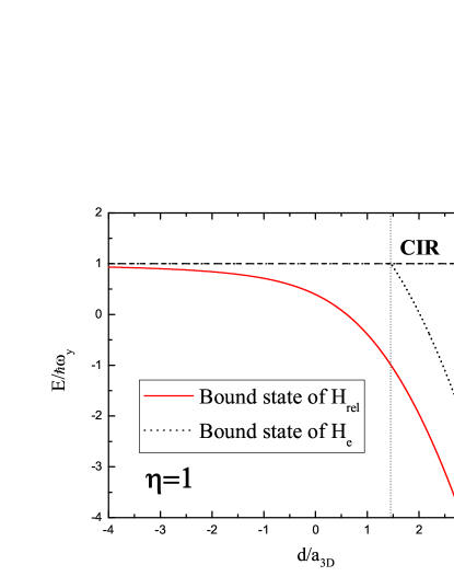
Figure 1: (Color online) The bound states of the total relative Hamiltonian $\hat{H}_{rel}$ (the solid curve) and the excited Hamiltonian $\hat{H}_{e}$ (the dotted curve) with $\eta=1$ .

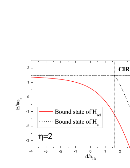
Figure 2: (Color online) The same as Fig.1 but for $\eta=2$ .

Bergeman, et al. Bergeman2003 show that the physical origin of the CIR is a zero-energy Feshbach resonance under tight transverse confinement. The ground transverse mode and the manifold of excited modes play the roles of the open channel and the closed channel, respectively. If a bound state exists in the closed channel, a resonance will occur when the bound-state energy is equal to the incident energy of two colliding atoms in the ground transverse mode of the total Hamiltonian. In this section, we calculate the bound state of the decoupled excited manifold. We find that a resonace will appear at $a_{3D}^{(R)}/a_{y}=\sqrt{2}/{\cal C}$, consistent with the calculations in Sec.II.1.

Using a similar method to Sec.II.1, the wavefunction of the total relative Hamiltonian $\hat{H}_{rel}$ can be expanded in terms of the eigenstates of the non-interacting Hamiltonian, Eq.(6). After substituting Eq.(6) into the Schroedinger equation and using the normalization and orthogonality of the wavefunctions, we arrive at,

$$\left[\frac{\partial}{\partial r}r\mathcal{H}\left(\vec{r}\right)\right]_{r=0}=-\frac{1}{2\pi a_{3D}d^{2}}$$ (20)

where

$$\mathcal{H}\left(\vec{r}\right)=\int_{-\infty}^{\infty}\frac{dk_{z}}{2\pi}\sum_{n_{1}=0}^{\infty}\sum_{n_{2}=0}^{\infty}\frac{e^{ik_{z}z}\phi_{n_{1}}^{*}\left(0\right)\phi_{n_{2}}^{*}\left(0\right)\phi_{n_{1}}\left(x\right)\phi_{n_{2}}\left(y\right)}{\frac{1}{2}d^{2}k_{z}^{2}+n_{1}\eta+n_{2}-\epsilon}$$ (21)

and $\epsilon=E/\hbar\omega_{y}-\eta/2-1/2$ . Using

$$\frac{1}{n}=\int_{0}^{1}dqq^{n-1}\qquad\left(n>0\right)$$ (22)

and

$$\sum_{k=0}^{\infty}\frac{t^{k}}{2^{k}k!}H_{k}(x)H_{k}(y)=\frac{exp(\frac{2txy-t^{2}x^{2}-t^{2}y^{2}}{1-t^{2}})}{\sqrt{1-t^{2}}}\,,$$ (23)

Eq.(21) can be written as

$$\mathcal{H}\left(\vec{r}\right) = \frac{\eta^{1/2}}{2\pi^{3/2}d^{3}}exp\left[-\frac{1}{2d^{2}}\left(\eta x^{2}+y^{2}\right)\right]\times$$ (24)

$$\int_{0}^{\infty}dt\frac{exp\left[\frac{t\epsilon}{2}-\frac{1}{t}\frac{z^{2}}{d^{2}}\right]}{\sqrt{t}}\frac{exp\left[-\frac{\eta e^{-\eta t}x^{2}}{\left(1-e^{-\eta t}\right)d^{2}}\right]}{\sqrt{1-e^{-\eta t}}}\times$$

$$\frac{exp\left[-\frac{e^{-t}y^{2}}{\left(1-e^{-t}\right)d^{2}}\right]}{\sqrt{1-e^{-t}}}$$

for $\epsilon<0$ . As $r\rightarrow 0$ , only the small $t$ terms dominate the integral, so that

$$\mathcal{H}\left(r\rightarrow 0\right) = \frac{\eta^{1/2}}{2\pi^{3/2}d^{3}}\int_{0}^{\infty}dt\frac{exp\left[-\frac{r^{2}}{td^{2}}\right]}{\eta^{1/2}t^{3/2}}$$ (25)

$$= \frac{1}{2\pi d^{2}r}\,.$$

Hence, the function $\mathcal{H}\left(\vec{r}\right)$ can be rewritten as,

$$\mathcal{H}\left(\vec{r}\right)=\frac{1}{2\pi^{3/2}d^{3}}\mathcal{F}\left(\epsilon,\vec{r}\right)+\frac{1}{2\pi d^{2}r}$$ (26)

and the regular part $\mathcal{F}\left(\epsilon,\vec{r}\right)$ has the form,

$$\mathcal{F}\left(\epsilon,\vec{r}\right) = exp\left[-\frac{1}{2d^{2}}\left(\eta x^{2}+y^{2}\right)\right]\times$$ (27)

$$\int_{0}^{\infty}dt\left\{\frac{\sqrt{\eta}exp\left[\frac{t\epsilon}{2}-\frac{1}{t}\frac{z^{2}}{d^{2}}\right]}{\sqrt{t}}\frac{exp\left[-\frac{\eta e^{-\eta t}x^{2}}{\left(1-e^{-\eta t}\right)d^{2}}\right]}{\sqrt{1-e^{-\eta t}}}\times\right.$$

$$\frac{exp\left[-\frac{e^{-t}y^{2}}{\left(1-e^{-t}\right)d^{2}}\right]}{\sqrt{1-e^{-t}}}-\left.\frac{exp\left[-\frac{r^{2}}{td^{2}}\right]}{t^{3/2}}\right\}\,.$$

Next, from Eq.(20), we obtain,

$$\mathcal{F}\left(\epsilon,0\right)=-\frac{\sqrt{\pi}d}{a_{3D}}$$ (28)

where

$$\mathcal{F}\left(\epsilon,0\right)=\int_{0}^{\infty}dt\left\{\frac{\sqrt{\eta}exp\left(\frac{t\epsilon}{2}\right)}{\sqrt{t\left(1-e^{-\eta t}\right)\left(1-e^{-t}\right)}}-\frac{1}{t^{3/2}}\right\}$$ (29)

for $\epsilon<0$ . Eq.(28) and (29) determine the bound-state energy of the total relative Hamiltonian depending on the interaction strength, which is denoted by the 3D scattering length $a_{3D}$ .

If the transverse ground state is projected out from the Hilbert space, we can define the excited Hamiltonian as,

$$\hat{H}_{e}\equiv\hat{H}_{rel}-\hat{P_{g}}\hat{H}_{rel}\hat{P}_{g}$$ (30)

where $\hat{P}_{g}=\left|g\right\rangle\left\langle g\right|$ is the projection operator of the transverse ground mode $\left|g\right\rangle$ . We can also calculate the bound-state energy of the excited Hamiltonian $\hat{H}_{e}$ by removing the $n_{1}=n_{2}=0$ term from the summation of the function $\mathcal{H}\left(\vec{r}\right)$ , i.e., Eq.(21). Then the bound-state energy of the excited Hamiltonian $\hat{H}_{e}$ should be determined by,

$$\left[\frac{\partial}{\partial r}r\mathcal{H}_{e}\left(\vec{r}\right)\right]_{r=0}=-\frac{1}{2\pi a_{3D}d^{2}}$$ (31)

where

$$\mathcal{H}_{e}\left(\vec{r}\right) = \mathcal{H}\left(\vec{r}\right)-\frac{L\sqrt{\eta}}{\sqrt{2}\pi d^{3}\sqrt{-\epsilon}}exp\left[-\frac{1}{2d^{2}}\left(\eta x^{2}+y^{2}\right)\right]\times$$ (32)

$$exp\left(-\sqrt{-2\epsilon}\frac{\left|z\right|}{d}\right)$$

for $\epsilon<0$ . Consequently, we can redefine the regular part of $\mathcal{H}_{e}\left(\vec{r}\right)$ as

$$\mathcal{F}_{e}\left(\epsilon,\vec{r}\right) = \mathcal{F}\left(\epsilon,\vec{r}\right)-\sqrt{\frac{2\pi\eta}{-\epsilon}}exp\left[-\frac{1}{2d^{2}}\left(\eta x^{2}+y^{2}\right)\right]\times$$ (33)

$$exp\left(-\sqrt{-2\epsilon}\frac{\left|z\right|}{d}\right)\,.$$

Then, using Eq.(31) and (33), we arrive at

$$\mathcal{F}_{e}\left(\epsilon,0\right)=-\frac{\sqrt{\pi}d}{a_{3D}}$$ (34)

where

$$\mathcal{F}_{e}\left(\epsilon,0\right) = \int_{0}^{\infty}dt\left\{\frac{exp\left(\frac{t\epsilon}{2}\right)\sqrt{\eta}}{\sqrt{t}}\times\right.$$

$$\left.\left[\frac{1}{\sqrt{\left(1-e^{-\eta t}\right)\left(1-e^{-t}\right)}}-1\right]-\frac{1}{t^{3/2}}\right\}\,.$$

This determines the bound-state energy of the excited Hamiltonian $\hat{H}_{e}$ .

For isotropic confinement ($\eta=1$), it is obvious that,

$$\mathcal{F}_{e}\left(\epsilon,0\right)=\mathcal{F}\left(\epsilon-2\hbar\omega,0\right)$$ (35)

Hence, from Eq.(28) and (34), the bound state of the excited Hamiltonian $\hat{H}_{e}$ is $2\hbar\omega$ higher than that of the total relative Hamiltonian $\hat{H}_{rel}$ , which is consistent with the conclusion of Bergeman Bergeman2003 .

The bound states of the total relative Hamiltonian $\hat{H}_{rel}$ and the excited Hamiltonian $\hat{H}_{e}$ are plotted as functions of the 3D scattering length $a_{3D}$ in Fig.1 and Fig.2 with transverse aspect ratios $\eta=1$ and $\eta=2$ for isotropic and the anisotropic confinement, respectively. It is obvous that there is only one bound state for the excited Hamiltonian $\hat{H}_{e}$ both for isotropic and anisotropic confinement. A confinement-induced resonance occurs when this bound state becomes degenerate with the threshold of the transverse ground mode of the total relative Hamiltonian. The position of the CIR in terms of the 3D scattering length is determined by Eq.(34) with $\epsilon=0$,

$$\frac{d}{a_{3D}^{(R)}} = -\frac{1}{\sqrt{\pi}}\int_{0}^{\infty}dt\left\{\frac{\sqrt{\eta}}{\sqrt{t}}\left[\frac{1}{\sqrt{\left(1-e^{-\eta t}\right)\left(1-e^{-t}\right)}}-1\right]\right.$$ (36)

$$\left.-\frac{1}{t^{3/2}}\right\}$$

$$\equiv {\cal C}.$$

This result is consistent with that in the Sec.II.1 which is $(a_{3D}^{(R)}/a_{y})=\sqrt{2}/{\cal C}$.

III Results and discussions

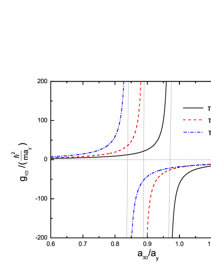
Figure 3: (Color online) The effective 1D coupling constant, $g_{1D}$ (in units of $\hbar^{2}/(ma_{y})$), as a function of $a_{3D}/a_{y}$ at different transverse anisotropy $\eta=1$ (solid line), $1.5$ (dashed line), and $3$ (dot-dashed line).

We plot in Fig.3 the effective 1D coupling constant as a function of the 3D s-wave scattering length at $\eta=1$, $1.5$, and $3$. In this parameter range, with increasing transverse anisotropy, the resonance position of CIR shifts from $(a_{3D}/a_{y})_{\eta=1}^{(R)}=\sqrt{2}{\cal C}_{\eta=1}^{-1}=0.9684...$ to lower values. For the experimental situation with a 3D scattering length tuned by a magnetic Feshbach resonance, this decrease corresponds to a shift to the deep BEC side of the Feshbach resonance.

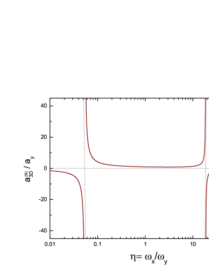
Figure 4: (Color online) Resonance positions of CIR, $a_{3D}^{(R)}/a_{y}$, as a function of the transverse anisotropy $\eta=\omega_{x}/\omega_{y}$. For sufficient large or small values of transverse anisotropy, the quasi-1D system crosses over to the quasi-2D regime.

In a wider parameter space, however, we observe an interesting non-monotonic behavior of the resonance position as a function of the ratio $\eta$. As shown in Fig.4, at sufficiently large (or small) values of the transverse anisotropy $\eta$, the resonance position $a_{3D}^{(R)}$ increases with increasing (or decreasing) transverse anisotropy, and diverges at a critical frequency ratio $\eta_{0}\simeq 18.551$ (or $\eta_{0}^{-1}\simeq 0.0539$). For $a_{3D}^{(R)}$, this corresponds to a bend-back to the magnetic Feshbach resonance from the BEC limit. On further increasing (or decreasing) the transverse anisotropy, the quasi-1D quantum gas crosses over to a pancake-shaped, horizontally-oriented 2D system, which would lead to a negative value for $a_{3D}^{(R)}$. This observation is in agreement with theoretical calculationsNaidon2007 showing that for a quasi-2D system, the $s$-wave CIR occurs always at a negative 3D scattering length ($a_{3D}<0$) or on the BCS side of the magnetic Feshbach resonance.

We now compare our theoretical results with the experimental data Haller2010 . This experiment uses a narrow Feshbach resonance in ${}^{133}Cs$ Kraemer2004 , together with a nonadiabatic jump to a particular magnetic field to initiate the resonance with a finite kinetic energy. As a result, one may expect some differences to the simplest single-channel model used here. The single-channel model does not include the molecular field corresponding to the bound molecule state. It is known from both mean-field Diener2004 and beyond mean-field xiajiggtheory calculations that, the single-channel model describes only a broad Feshbach resonance. As illustrated in Fig.5, our prediction of $a_{3D}^{(R)}$ is just between the two CIRs observed in the experiment, and disagrees with either of them. In fact, the observation of a single CIR s-wave resonance in our theoretical calculation can be easily understood. Recall that the CIR is a kind of Feshbach resonance, which occurs when the scattering state in an open channel becomes degenerate in energy with the bound states in the closed channel. The number of CIRs is therefore simply equal to the number of bound states in the closed channel. For a quasi-1D quantum gas, the excited transverse modes are grouped together and regarded as closed channels (see, for example, ref. Bergeman2003 for a detailed discussion of closed channels). In our model, the sub-Hilbert space of the excited transverse modes can only sustain a single bound state, no matter how large large the transverse anisotropy is. The experimental observation of two resonances must therefore have a different origin than the simple zero-energy s-wave scattering picture pursued in this work.

Interestingly, we obtain a good agreement with experimental data if we include in the resonance condition an additional factor of $\sqrt{\eta}$. As shown in Fig. 5, the CIR₁ and CIR₂ resonances are well reproduced theoretically if we use the conditions, $a_{3D}^{(R)}/a_{y}=\sqrt{2\eta}/\mathcal{C}$ and $a_{3D}^{(R)}/a_{y}=\sqrt{2/\eta}/\mathcal{C}$, respectively. This additional factor however can not justified.

It should be note that, by keeping $\omega_{x}$ invariant and weakening the confinement $\omega_{y}$ - which therefore gives an alternative way to increase the value of $\eta$ - the observed CIR₁ displays additional structure. It further splits into many sub-resonances at $\eta>1.5$ and finally disappears at sufficiently large values of transverse anisotropy. At the same time the CIR₂ persists. Also, in the limit of a 2D system ($\eta\rightarrow\infty$), the resonance position of the surviving CIR₂ is at a positive 3D scattering length. These experimental observations also disagree with our simple zero-energy s-wave scattering calculation, and with previous calculationsNaidon2007 of 2D s-wave CIR. One possibility is that many-body physics of the quantum bosonic gas may come into play. A likely explanation therefore is that the CIRs observed in this experiment are associated with the failure of Olshanii’s model Olshanii1998 which is only a zero-energy single-channel s-wave description of the inter-atomic interactions, and the experimental conditions are different to this simple model. An advanced theory of CIRs need to be introduced, e.g., multi-channel scattering theory including molecular channels, non-zero collision energy theory, or many-body effects.

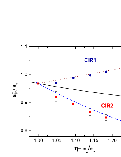
Figure 5: (Color online) Resonance positions of CIRs, obtained by solving $a_{3D}^{(R)}/a_{y}=\sqrt{2}/\mathcal{C}$, as a function of the transverse anisotropy $\eta=\omega_{x}/\omega_{y}$. The experimental results (symbols) are compared with our zero-energy s-wave scattering prediction (solid line). In the presence of transverse anisotropy, it is difficult to determine directly the resonance positions from atom loss. Therefore, experimentally the positions were obtained by determining the associated atom number minima and then subtracting a constant offset. In accord with this procedure, we have uniformly offset the experimental data in such a way that the measured resonance position in the symmetric limit ($\eta=1$) is equal to the known theoretical prediction by Olshanii Olshanii1998 . The dashed and dot-dashed lines are the resonance positions, obtained respectively by solving, $a_{3D}^{(R)}/a_{y}=\sqrt{2\eta}/\mathcal{C}$ and $a_{3D}^{(R)}/a_{y}=\sqrt{2/\eta}/\mathcal{C}$. See the text for more details.

IV Conclusions and remarks

In conclusion, we have presented a theoretical calculation of confinement-induced resonance (CIR) under transversely anisotropic confinement, by extending the standard zero-energy s-wave scattering approach to incorporate transverse anisotropy. We have theoretically found a single CIR and have explained its physical origin. The position of our predicted CIR disaggrees with either of the two CIRs measured most recently in a quasi-1D quantum bosonic gas of ${}^{133}Cs$ atoms. Therefore, the CIRs observed in the experiment cannot be explained simply by the zero-energy s-wave scattering theory. There are also several discrepancies when the quasi-1D system crosses over to the quasi-2D regime, which may arise either from the many-body physics of Cs atoms, or the residual molecular fraction and angular momentum of the magnetic Feshbach resonance. To take these aspects into account, we look forward to improving the current s-wave scattering calculation by replacing the two-body scattering matrix with its many-body counterpart and/or adopting a two-channel model to describe the magnetic Feshbach resonance.

- (1) I. Bloch, J. Dalibard, and W. Zwerger, Rev. Mod. Phys. 80, 885 (2008).
- (2) H. Hu, X.-J. Liu, and P. D. Drummond, Phys. Rev. Lett. 98, 070403 (2007).
- (3) X.-J. Liu, H. Hu, and P. D. Drummond, Phys. Rev. A 76, 043605 (2007).
- (4) X.-J. Liu, H. Hu, and P. D. Drummond, Phys. Rev. A 78, 023601 (2008).
- (5) X.-J. Liu, H. Hu, and P. D. Drummond, Phys. Rev. A 77, 013622 (2008).
- (6) D. S. Petrov, G. V. Shlyapnikov, and J. T. M. Walraven, Phys. Rev. Lett. 85, 3745 (2000).
- (7) Z. Hadzibabic, P. Krüger, M. Cheneau, B. Battelier, J. Dalibard, Nature 441, 1118 (2006).
- (8) H. Feshbach, Ann. Phys. 19, 287 (1962).
- (9) T. Koehler, K. Goral, and P. S. Julienne, Rev. Mod. Phys. 78, 1311 (2006).
- (10) M. Olshanii, Phys. Rev. Lett. 81, 938 (1998).
- (11) T. Bergeman, M. G. Moore, and M. Olshanii, Phys. Rev. Lett. 91, 163201(2003).
- (12) J. I. Kim, J. Schmiedmayer, and P. Schmelcher, Phys. Rev. A 72, 042711(2005).
- (13) C. Mora, R. Egger, and A. O. Gogolin, Phys. Rev. A 71, 052705 (2005).
- (14) P. Naidon, E. Tiesinga, W. F. Mitchell, and P. S Julienne, New J. Phys. 9, 19 (2007).
- (15) S. Saeidian, V. S. Melezhik, and P. Schmelcher, Phys. Rev. A 77, 042721 (2008).
- (16) T. Kinoshita, T. Wenger, and D. S. Weiss, Science 305, 1125 (2004).
- (17) B. Paredes, A. Widera, V. Murg, O. Mandel, S. Fölling, I. Cirac, G. V. Shlyapnikov, T. W. Hänsch, and I. Bloch, Nature 429, 277 (2004).
- (18) K. Günter, T. Stöferle, H. Moritz, M. Köhl, and T. Esslinger, Phys. Rev. Lett. 95, 230401(2005).
- (19) E. Haller, M. Gustavsson, M. J. Mark, J. G. Danzl, R. Hart, G. Pupillo, and H.-C. Nägerl, Science 325, 1224 (2009).
- (20) E. Haller, M. J. Mark, R. Hart, J. G. Danzl, L. Reichsöllner, V. Melezhik, P. Schmelcher, and H.-C. Nägerl, Phys. Rev. Lett. 104, 153203(2010).
- (21) T. Busch, B.-G. Englert, K. Rzażewski, and M. Wilkens, Found. Phys. 28, 549 (1998).
- (22) Z. Idziaszek and T. Calarco, Phys. Rev. A 74, 022712 (2006).
- (23) J.-J. Liang and C. Zhang, Phys. Scr. 77, 025302 (2008).
- (24) T. Kraemer, J. Herbig, M. Mark, T. Weber, C. Chin, H.-C. Nagerl and R. Grimm, App. Phys. B 79, 1013 (2004).
- (25) R. B. Diener and T.-L. Ho, arXiv:0405174 (2004).
- (26) X.-J. Liu and H. Hu, Phys. Rev. A 72, 063613 (2005).