Cavitation and thermal photon production in relativistic heavy ion collisions

Abstract

We investigate the thermal photon production-rates using one dimensional boost-invariant second order relativistic hydrodynamics to find proper time evolution of the energy density and the temperature. The effect of bulk-viscosity and non-ideal equation of state are taken into account in a manner consistent with recent lattice QCD estimates. It is shown that the non-ideal gas equation of state i.e $\varepsilon-3\,P\,\neq 0$ behaviour of the expanding plasma, which is important near the phase-transition point, can significantly slow down the hydrodynamic expansion and thereby increase the photon production-rates. Inclusion of the bulk viscosity may also have similar effect on the hydrodynamic evolution. However the effect of bulk viscosity is shown to be significantly lower than the non-ideal gas equation of state. We also analyze the interesting phenomenon of bulk viscosity induced cavitation making the hydrodynamical description invalid. It is shown that ignoring the cavitiation phenomenon can lead to a very significant over estimation of the photon flux. It is argued that this feature could be relevant in studying signature of cavitation in relativistic heavy ion collisions.

I INTRODUCTION

Thermal photons emitted from the hot fireball created in relativistic heavy-ion collisions is a promising tool for providing a signature of quark-gluon plasma kapu91 ; baier92 ; Ruus92 ; thoma95 ; traxler95 ; arnoldJHEP (see Alam01R ; Peitz-Thoma:02R ; Gale:03R for recent reviews). Since they participate only in electromagnetic interactions, they have a larger mean free path compared to the transverse size of the hot and dense matter created in nuclear collisions kapusta . Therefore these photons were proposed to verify the existence of the QGP phase Feinberg76 ; Shyryak78 . Spectra of thermal photons depend upon the fireball temperature and they can be calculated from the scattering cross-section of the processes like $q\bar{q}\rightarrow g\gamma$, bremsstrahlung etc. Time evolution of the temperature can be calculated using hydrodynamics with appropriate initial conditions. Thus the spectra depend upon the equation of state (EoS) of the medium and they may be useful in finding a signature of the quark-gluon plasmadk99:EPJC ; thoma07 ; dkdir08 ; Liu09 . Recently the thermal photons are proposed as a tool to measure the shear viscosity of the strongly interacting matter produced in the collisionsskv-photon ; dusling09 .

Understanding shear viscosity of QGP is one of the most intriguing aspects of the experiments at Relativistic Heavy Ion Collider (RHIC). Analysis of the experimental data collected from RHIC show that the strongly coupled matter produced in the collisions is not too much above the phase transition temperature $T_{c}$ and it may have extremely small value of shear viscosity $\eta$. In fact the ratio of the shear viscosity $\eta$ to the entropy density $s$ i.e. $\eta/s$ is around $1/4\pi$ which is the smallest for any known liquid in the natureSchf-Teaney-09R . In fact the arguments based on AdS-CFT suggest that the values of $\eta/s$ can not become lower than $1/4\pi$. This is now known as Kovtun-Son-Starinets or ’KSS- bound’ kss05 . Thus the quark-gluon plasma produced in RHIC experiments is believed to be in a form of the most perfect liquidHirano:2005wx . No wonder ideal hydrodynamic appears to be best description of such matter as suggested by comparison between the experimental dataRHIC and the calculations done using second-order relativistic hydrodynamics BR07 ; rom:PRL ; DT08 ; hs08 ; LR08 ; Molnar08 ; Song:2008hj ; LR09 .

However there remains uncertainties in understanding the application and validity of the hydrodynamical procedure in the relativistic heavy-ion collision experiments. It is only very recently realized that the effect of bulk viscosity can bring complications in the hydrodynamical description of the heavy-ion collisions. Generally it was believed that the bulk viscosity does not play a significant role in the hydrodynamics of relativistic heavy-ion collisions. It was argued that that since $\zeta$ scaled like $\varepsilon-3P$ at very high energy the bulk viscosity may not play a significant role because the matter might be following the ideal gas type equation of statewein . But during its course of expansion the fireball temperature can approach values close to $T_{c}$. Recent lattice QCD results may not have ideal gas EoS and the ratio $\zeta/s$ show a strong peak around $T_{c}$ Bazavov:2009 ; Meyer:2008 . The bulk viscosity contribution in this regime can be much larger than that of the the shear viscosity. Recently the role of bulk viscosity in heating and expansion of the fireball was analyzed using one dimensional hydrodynamicsfms08 . Another complication that bulk viscosity brings in hydrodynamics of heavy-ion collisions is phenomenon of cavitationkr:2010cv . Cavitation arises when the fluid pressure becomes smaller than the vapour pressure. Since the bulk viscosity (and also shear viscosity) contributes to the pressure gradient with a negative contribution, it may be possible for the effective fluid pressure to become zero. Once the cavitation sets in the hydrodynamical description breaks down. It was shown in Ref.kr:2010cv that cavitation may happen in RHIC experiments when the effect of bulk viscosity is included in manner consistent with the lattice results. It was shown that the cavitation may significantly reduce the time of hydrodynamical evolution.

One of the main objectives of this paper is to study the photon spectra with the effect of bulk viscosity and cavitation. Finite $\zeta$ effect can either significantly reduce the time for the hydrodynamical evolution (by onset of cavitation) or it can increase the time by which the system reaches $T_{c}$! Moreover the non-ideal gas EoS can also significantly influence the hydrodynamics (see below). In what follows, we use equations of relativistic second order hydrodynamics to incorporate the effects of finite viscosity. We take the value of $\zeta/s$ same as that in Ref.kr:2010cv and keep $\eta/s=1/4\pi$. Further we use one dimensional boost invariant hydrodynamics in the same spirit as in Refs.fms08 ; kr:2010cv . One of the limitations of this approach is that the effects of transverse flow cannot be incorporated. As the boost-invariant hydrodynamics is known to lead to underestimation of the effects of bulk viscosityfms08 , we believe that our study of the photon spectra will provide a conservative estimate of the effect.

II FORMALISM

II.1 Viscous Hydrodynamics

We represent the energy momentum tensor of the dissipative QGP formed in high energy nuclear collisions as

$$T^{\mu\nu}=\varepsilon\,u^{\mu}\,u^{\nu}\,-P\,\Delta^{\mu\nu}+\Pi^{\mu\nu}$$ (1)

where $\varepsilon$, $P$ and $u^{\mu}$ are the energy density, pressure and four velocity of the fluid element respectively. The operator $\Delta^{\mu\nu}~{}=~{}g^{\mu\nu}-u^{\mu}\,u^{\nu}$ acts as a projection perpendicular to four velocity. The viscous contributions to $T^{\mu\nu}$ are represented by

$$\Pi^{\mu\nu}=\pi^{\mu\nu}-\,\Delta^{\mu\nu}\,\Pi$$ (2)

where $\pi^{\mu\nu}$, the traceless part of $\Pi^{\mu\nu}$; gives the contribution of shear viscosity and $\Pi$ gives the bulk contribution. The corresponding equations of motion are given by,

$$D\varepsilon+(\varepsilon+P)\,\theta-\Pi^{\mu\nu}\nabla_{(\mu}\,u_{\nu)}=0$$ (3)

$$(\varepsilon+P)\,Du^{\alpha}-\nabla^{\alpha}P\,+\,\Delta_{\alpha\nu}\,\partial_{\mu}\Pi^{\mu\nu}=0$$ (4)

where $D\equiv u^{\mu}\partial_{\mu}$, $\theta\equiv\partial_{\mu}\,u^{\mu}$, $\nabla_{\alpha}=\Delta_{\mu\alpha}\partial^{\mu}$ and $A_{(\mu}\,B_{\nu)}=\frac{1}{2}[A_{\mu}\,B_{\nu}+A_{\nu}\,B_{\mu}]$ gives the symmetrization.

We employ Bjorken’s prescriptionbjor to describe the one dimensional boost invariant expanding flow, were we use the convenient parametrization of the coordinates using the proper time $\tau=\sqrt{t^{2}-z^{2}}$ and space-time rapidity $y=\frac{1}{2}\,ln[\frac{t+z}{t-z}]$; $t=\tau$ cosh$\,y$ and $z=\tau$ sinh$\,y$. Then the four velocity is given by,

$$u^{\mu}=(\rm{cosh}\,y,0,0,\rm{sinh}\,y).$$ (5)

We note that with this transformation of the coordinates, $D=\frac{\partial\,}{\partial\tau}$ and $\theta=1/\tau$.

Form of the energy momentum tensor in the local rest frame of the fireball is then given byTeaney03 ; SHC06 ; AM07 ; AM-prl02

$$T^{\mu\nu}=\left(\begin{array}[]{cccc}\varepsilon&0&0&0\\ 0&P_{\perp}&0&0\\ 0&0&P_{\perp}&0\\ 0&0&0&P_{z}\end{array}\right)$$ (6)

where the effective pressure of the expanding fluid in the transverse and longitudinal directions are respectively given by

$$P_{\perp} = P+\Pi+\frac{1}{2}\Phi$$

$$P_{z} = P+\Pi-\Phi$$ (7)

Here $\Phi$ and $\Pi$ are the non-equilibrium contributions to the equilibrium pressure $P$ coming from shear and bulk viscosities. Respecting the symmetries in the transverse directions the traceless shear tensor has the form $\pi^{ij}=\mathrm{diag}(\Phi/2,\Phi/2,-\Phi)$.

In the first order Navier-Stokes dissipative hydrodynamics

$$\Pi=-\zeta\partial_{\mu}u^{\mu}\quad\rm{and}\quad\pi^{\mu\nu}=2\eta\nabla^{\langle\mu}u^{\nu\rangle}\,,$$ (8)

with $\zeta,\eta>0$ and $\nabla_{\langle\mu}u_{\nu\rangle}=2\nabla_{(\mu}\,u_{\nu)}-\frac{2}{3}\,\Delta_{\mu\nu}\nabla_{\alpha}u^{\alpha}$. So for first order theories with Bjorken flow we have

$$\Pi=-\frac{\zeta}{\tau}\quad\rm{and}\quad\Phi=\frac{4\eta}{3\tau}.$$ (9)

The Navier-Stokes hydrodynamics is known to have instabilities and acausal behaviourslindblom ; BRW-06 ; second order theories removes such unphysical artifacts.

We use causal dissipative second order hydrodynamics of Isreal-StrewartIsrael:1979wp to study the expanding plasma in the fireball. In this theory we have evolution equations for $\Pi$ and $\Phi$ governed by their relaxation times $\tau_{\Pi}$ and $\tau_{\pi}$. We refer AM-DR:04 ; ROM:09R for more details on the recent developments in the theory and its application to relativistic heavy ion collisions.

Under these assumptions, the set of equations (i.e., equation of motion (3) and relaxation equations for viscous terms) dictating the longitudinal expansion of the medium are given byAM07 ; BRW-06 ; Heinz05

$$\frac{\partial\varepsilon}{\partial\tau} = -\frac{1}{\tau}(\varepsilon+P+\Pi-\Phi)\,,$$ (10)

$$\frac{\partial\Phi}{\partial\tau} = -\frac{\Phi}{\tau_{\pi}}+\frac{2}{3}\frac{1}{\beta_{2}\tau}-\left[\frac{4\tau_{\pi}}{3\tau}\Phi+\frac{\lambda_{1}}{2\eta^{2}}\Phi^{2}\right]\,,$$ (11)

$$\frac{\partial\Pi}{\partial\tau} = -\frac{\Pi}{\tau_{\Pi}}-\frac{1}{\beta_{0}\tau}.$$ (12)

where $\Phi=\pi^{00}-\pi^{zz}$. The terms in the square bracket in Equation(11) are needed for the conformality of the theoryBaier:2008:JHEP . The coefficients $\beta_{0}$ and $\beta_{2}$ are related with the relaxation time by

$$\tau_{\Pi}=\zeta\,\beta_{0}\,,\tau_{\pi}=2\eta\,\beta_{2}.$$ (13)

We use the $\mathcal{N}\,=\,4$ supersymmetric Yang-Mills theory expressions for $\tau_{\pi}$ and $\lambda_{1}$ Baier:2008:JHEP ; Okamura:N=4 ; shiraz:N=4 :

$$\tau_{\pi}=\frac{2-\ln 2}{2\pi T}$$ (14)

and

$$\lambda_{1}=\frac{\eta}{2\pi T}\,.$$ (15)

We set $\tau_{\pi}(T)=\tau_{\Pi}(T)$ as we don’t have any reliable prediction for $\tau_{\Pi}$fms08 .

In order to close the hydrodynamical evolution equations (10 - 12) we need to supply the equation of state.

II.2 Equation of state, $\zeta/s$ and $\eta/s$

We are interested in the effect of bulk viscosity on the hydrodynamical evolution of the plasma and recent studies show that near the critical temperature $T_{c}$ effect of bulk viscosity becomes importantkarsch07 ; Kharzeev:2007wb . We use the recent lattice QCD result of A. Bazavov $\it{et~{}al.}$Bazavov:2009 for equilibrium equation of state (EoS) (non-ideal: $\varepsilon-3P\neq 0$). Parametrised form of their result for trace anomaly is given by

$$\frac{\varepsilon-3P}{T^{4}}=\left(1-\frac{1}{\left[1+\exp\left(\frac{T-c_{1}}{c_{2}}\right)\right]^{2}}\right)\left(\frac{d_{2}}{T^{2}}+\frac{d_{4}}{T^{4}}\right)\ ,$$ (16)

where values of the coefficients are $d_{2}=0.24$ GeV², $d_{4}=0.0054$ GeV⁴, $c_{1}=0.2073$ GeV, and $c_{2}=0.0172$ GeVkr:2010cv . Their calculations predict a cross over from QGP to hadron gas around .200-.180 GeV. We take critical temperature as .190 GeV throughout the analysis. The functional form of the pressure is given by Bazavov:2009

$$\frac{P(T)}{T^{4}}-\frac{P(T_{0})}{T_{0}^{4}}=\int_{T_{0}}^{T}dT^{\prime}\,\frac{\varepsilon-3P}{T^{\prime 5}}\ ,$$ (17)

with $T_{0}~{}$= 50 MeV and $P(T_{0})$ = 0 kr:2010cv .

From Equations (16) and (17) we get $\varepsilon$ and $P$ in terms of $T$.

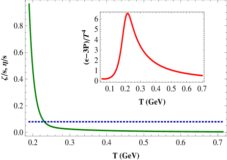
Figure 1: $(\varepsilon-3P)/T^{4}\,,\zeta/s$ (and $\eta/s=1/4\pi$) as functions of temperature T. One can see around critical temperature ($T_{c}=.190$ GeV) $\zeta\gg\eta$ and departure of equation of state from ideal case is large.

We rely upon the lattice QCD calculation results for determining $\zeta/s$. We use the result of MeyerMeyer:2008 , which indicate the existence a peak of $\zeta/s$ near $T_{c}$, however the height and width of this curve are not well understood. We follow parametrization of Meyer’s result from Ref.kr:2010cv , given by

$$\frac{\zeta}{s}=a\exp\left(\frac{T_{c}-T}{\Delta T}\right)+b\left(\frac{T_{c}}{T}\right)^{2}\quad{\rm for}\ T>T_{c},$$ (18)

where $b$ = 0.061. The parameter $a$ controls the height and $\Delta T$ controls the width of the $\zeta/s$ curve and are given by

$$a=0.901,\,\Delta T=\frac{T_{c}}{14.5}.$$ (19)

We will change these values to explore the various cases of $\zeta/s$ to account for the uncertainty of the height and width of the curve. In FIG.2 we show the change in bulk viscosity profile by varying the width of the $\zeta/s$ curve by keeping the height intact.

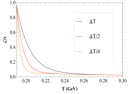
Figure 2: Various bulk viscosity scenarios by changing the width of the curve through the parameter $\Delta T$.

We use the lower bound of the shear viscosity to entropy density ratio known as KSS boundkss05

$$\eta/s=1/4\pi$$ (20)

in our calculations. We note that the entropy density is obtained from the relation

$$s=\frac{\varepsilon+P}{T}.$$ (21)

In FIG.1 we plot the trace anomaly $(\varepsilon-3P)/T^{4}$ and $\zeta/s$ for desired temperature range. We also plot the constant value of $\eta/s=1/4\pi$ for a comparison. It is clear that the non-ideal EoS deviates from the ideal case ($\varepsilon=3P$) significantly around the critical temperature. Around same temperature $\zeta/s$ starts to dominate over $\eta/s$ significantly. We would like to note that these results are qualitatively in agreement with Ref.fms08 .

II.3 Thermal photons

During QGP phase thermal photons are originated from various sources, like Compton scattering $q(\bar{q})g\rightarrow q(\bar{q})\gamma$ and annihilation processes $q\bar{q}\rightarrow g\gamma$. Recently Aurenche et al. showed that two loop level bremsstrahlung process contribution to photon production is as important as Compton or annihilation contributions evaluated up to one loop levelaurenche:98 . They also discuss a new mechanism for hard photon production through the annihilation of an off-mass shell quark and an antiquark, with the off-mass shell quark coming from scattering with another quark or gluon. These processes in the context of hydrodynamics of heavy ion collisions were studied in Refs.dk99:EPJC ; thoma07 . Until recently only the processes of Compton scattering and $q\bar{q}$-annihilation were considered in studying the photon production rates.

The production rate for hard ($E>T$) thermal photons from equilibrated QGP evaluated to the one loop order using perturbartive thermal QCD based on hard thermal loop (HTL) resummation to account medium effects. The Compton scattering and $q\bar{q}$-annihilation contribution iskapu91 ; baier92 ; traxler95

$$E\frac{dN}{d^{4}xd^{3}p}~{}=~{}\frac{1}{2\pi^{2}}\alpha\alpha_{s}\left(\sum_{f}e_{f}^{2}\right)~{}T^{2}~{}e^{-E/T}~{}\rm{ln}\left(\frac{cE}{\alpha_{s}T}\right),$$ (22)

where the constant $c\approx$ 0.23 and $\alpha$ and $\alpha_{s}$ are the electromagnetic and strong coupling constants respectively. In summation $f$ denotes the flavours of the quarks and $e_{f}$ is the electric charge of the quark in units of the charge of the electron.

The rate of photon production due to Bremsstrahlung processes is given byaurenche:98

$$E\frac{dN}{d^{4}xd^{3}p}~{}=~{}\frac{8}{\pi^{5}}\alpha\alpha_{s}\left(\sum_{f}e_{f}^{2}\right)~{}\frac{T^{4}}{E^{2}}~{}e^{-E/T}~{}(J_{T}-J_{L})~{}I(E,T)$$ (23)

where $J_{T}\approx 1.11$ and $J_{L}\approx−1.06$ for two flavours and three colors of quarksthoma07 . The expression for $I(E,T)$ is given by

$$I(E,T)=\left[3\zeta(3)+\frac{\pi^{2}}{6}\frac{E}{T}+\left(\frac{E}{T}\right)^{2}\rm{ln}(2)+4~{}\rm{Li}_{3}\left(-e^{-|E|/T}\right)+2\left(\frac{E}{T}\right)\rm{Li}_{2}\left(-e^{-|E|/T}\right)-\left(\frac{E}{T}\right)^{2}~{}\rm{ln}\left(1+e^{-|E|/T}\right)\right]$$ (24)

and $\rm{Li}$ are the polylogarithmic functions given by

$$\rm{Li_{a}}(z)=\sum_{n=1}^{+\infty}\frac{z^{n}}{n^{a}}.$$

Now the rate due to $q\bar{q}$-annihilation with an additional scattering in the medium is given by,

$$E\frac{dN}{d^{4}xd^{3}p}~{}=~{}\frac{8}{3\pi^{5}}\alpha\alpha_{s}\left(\sum_{f}e_{f}^{2}\right)~{}E~{}T~{}e^{-E/T}~{}(J_{T}-J_{L}).$$ (25)

We use the parametrization of $\alpha_{s}(T)$ by Karschkarsch88 :

$$\alpha_{s}(T)=\frac{6\pi}{(33-2N_{f})~{}\rm{ln(8T/T_{c})}}$$ (26)

for our rate calculations. Here $N_{f}$ is the number of quark flavors in consideration.

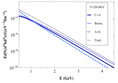
Figure 3: Hard thermal photon rates in QGP as a function of energy for a fixed temperature T=250 MeV. Photon rates are plotted for different relevant processes.

In Fig.3, we plot the different photon rates for a fixed temperature $T=250~{}MeV$. It shows the contributions from Bremsstrahlung (Brems), annihilation with scattering (A+S) and Compton scattering together with $q\bar{q}$-annihilation (C+A). Bremsstrahlung contributes to the photon production rate upto $E\sim 1~{}GeV$ only, afterwards A+S and C+A processes become dominant. This observation is in complete agreement with with Ref.thoma07 .

The total photon rate is obtained by adding different temperature depended photon rate expressions. Once the evolution of temperature is known from the hydrodynamical model, the total photon spectrum is obtained by integrating the total rate over the space time history of the collisionthoma ,

$$\left(\frac{dN}{d^{2}p_{\bot}dy}\right)_{y,p_{\bot}} = \int d^{4}x\left(E\frac{dN}{d^{3}pd^{4}x}\right)$$

$$= Q\int_{\tau_{0}}^{\tau_{1}}d\tau~{}\tau\int_{-y_{nuc}}^{y_{nuc}}dy^{{}^{\prime}}\left(E\frac{dN}{d^{3}pd^{4}x}\right)$$

where $\tau_{0}$ and $\tau_{1}$ are the initial and final values of time we are interested. $y_{nuc}$ is the rapidity of the nuclei whereas $Q$ is its transverse cross-section. For a $Au$ nucleus $Q\sim 180fm^{2}$. $p_{\bot}$ is the photon momentum in direction perpendicular to the collision axis. The quantity $\left(E\frac{dN}{d^{3}pd^{4}x}\right)$ is Lorentz invariant and it is evaluated in the local rest frame in equation (II.3). Now the photon energy in this frame, i.e., in the frame comoving with the plasma, is given as $p_{\bot}cosh(y-y^{\prime})$. So once the rapidity and $p_{\bot}$ are given we get the total photon spectrum.

III RESULTS AND DISCUSSION

Table 1: Initial conditions for RHIC

$y_{nuc}$	$\tau_{0}$	$\rm{T_{0}}$
	$(fm/c)$	$(GeV)$
5.3	0.5	.310

In order to understand the temporal evolution of temperature $T(\tau)$, pressure $P(\tau)$ and viscous stresses - $\Phi(\tau)~{}\rm{and}~{}\Pi(\tau)$, we numerically solve the hydrodynamical equations describing the longitudinal expansion of the plasma: (10-12). We use the non-ideal EoS obtained from equations (16) and (17). Information about viscosity coefficients $\zeta$ and $\eta$ are obtained from equations (18-20) using equation (21). We need to specify the initial conditions to solve the hydrodynamical equations, namely the initial time $\tau_{0}$ and $T_{0}$. We use the initial values relevant for RHIC experiment given in Table I, taken from Ref.dk99:EPJC . We will take initial values of viscous contributions as $\Phi(\tau_{0})=0$ and $\Pi(\tau_{0})=0$. We would like to note that our hydrodynamical results are in complete agreement with that of Ref.kr:2010cv .

Once we get the temperature profile we calculate the photon production rates. Total photon spectrum $E\frac{dN}{d^{3}pd^{4}x}$ (as a function of rapidity, $y$ and transverse momentum of photon, $p_{\bot}$) is obtained by adding different photon rates using equations (22),(23),(25) and convoluting with the space time evolution of the heavy-ion collision with equation (II.3). The final value of time $\tau_{1}$ is the time at which temperature evolves to critical value $\tau_{f}$, i.e.; $T(\tau_{1})=T_{c}$. In all calculations we will consider the photon production in mid-rapidity region ($y=0$) only.

We will be exploring various values of viscosity and its effect on the system. Since there is an ambiguity regarding the height and width of $\zeta/s$ curve, we will vary the parameters $a~{}\rm{and}~{}\Delta T$ from its base value given in equation (19). By this we will able to study the effect of variation of $\zeta$ on the system. The varied values of the parameters are represented by $a^{\prime}~{}\rm{and}~{}\Delta T^{\prime}$. We note that unless specified we will be using the base values of bulk viscosity parameters (19) in our calculations. Throughout the analysis we will keep the shear viscosity $\eta$ to its base value given by equation (20).

In order to understand the effect of non-ideal EoS in hydrodynamical evolution and subsequent photon spectra we compare these results with that of an ideal EoS ($\varepsilon=3P$). We consider the EoS of a relativistic gas of massless quarks and gluons. The pressure of such a system is given by

$$P=a~{}T^{4}\,;\,a=\left(16+\frac{21}{2}N_{f}\right)~{}\frac{\,\pi^{2}}{90}$$ (28)

where $N_{f}=2$ in our calculations. Hydrodynamical evolution equations of such an EoS within ideal (without viscous effects) Bjorken flow can be solved analytically and the temperature dependence is given bybjor

$$T=T_{0}~{}\left(\frac{\tau_{0}}{\tau}\right)^{1/3},$$ (29)

where $\tau_{0}~{}\rm{and}~{}T_{0}$ are the initial time and temperature. While considering the viscous effect of this ideal EoS, we will solve the set of hydrodynamical equations (10 - 11), since effect of bulk viscosity can be neglected in the relativistic limit when the equation of state $P=\varepsilon/3$ is obeyed wein .

Hydrodynamics with non-ideal and ideal EoS

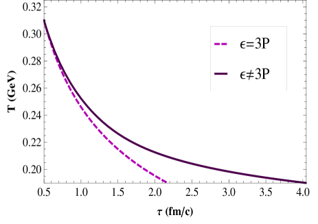
Figure 4: Temperature profile using massless (ideal) and non-ideal EoS in RHIC scenario. Viscous effects are neglected in both cases. System evolving with non-ideal EoS takes a significantly larger time to reach $T_{c}$ as compared to $ideal$ EoS scenario.

FIG. (4) shows plots of temperature versus time for the ideal and non-ideal equation of states. The temperature profiles are obtained from the hydrodynamics without incorporating the effect of viscosity. The figure shows system with non-ideal EoS takes almost the double time than the system with ideal massless EoS to reach $T_{c}$. So even when the effect of viscosity is not considered, inclusion of the non-ideal EoS makes significant change in temperature profile of the system. This can affect the corresponding photon production rates (below).

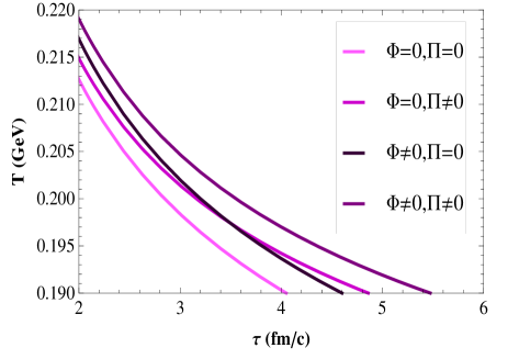
Figure 5: Figure shows time evolution of temperature with non-ideal EoS for different combinations of bulk ($\Pi$) and shear ($\Phi$) viscosities. Non zero value of bulk viscosity refers to equations (18-19) and non zero shear viscosity is calculated from equation (20).

Now we analyse the viscous effects. Role of shear viscosity in the boost invariant hydrodynamics of heavy ion collisions, for a chemically nonequilibrated system, was already considered in Ref.skv-photon .

Next we consider possible combinations of $\Phi$ and $\Pi$ in non-ideal EoS case and study the corresponding temperature profiles as shown in FIG. (5). As expected viscous effects is slowing down temperature evolution. For the case of non zero bulk and shear viscosities ($\Pi\neq 0;~{}\Phi\neq 0$), temperature takes the longest time to reach $T_{c}$ as indicated by the top most curve. This is $\sim 1.5~{}fm/c$ greater than the no viscosity case (the lowest curve). The remaining two curves show that the bulk viscosity dominates over the shear viscosity when the value of $T$ approaches $T_{c}$ and this makes the system to spend more time around $T_{c}$. However the intersection point of the two curves may vary with values of $a$ and $\Delta T$ as highlighted by FIG.2.

Non-ideal EoS and Cavitation

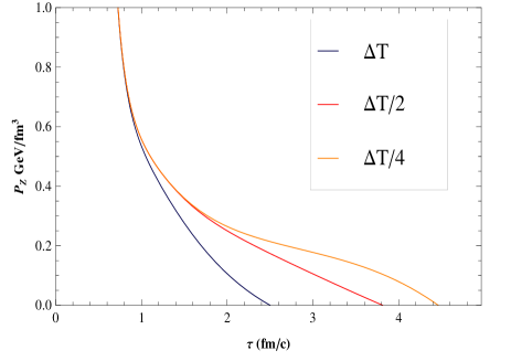
Figure 6: Longitudinal pressure $P_{z}$ for various viscosity cases shown in FIG.2.

Let us note the fact that $\Pi<0$ kr:2010cv . From the definition of longitudinal pressure $P_{z}=P+\Pi-\Phi$ it is clear that if either $\zeta$ ($\Pi$) or $\eta$ ($\Phi$) is large enough it can drive $P_{z}$ to negative values. $Pz=0$ defines the condition for the onset of cavitation. At this instant when of $P_{z}$ becoming zero the expanding fluid will break apart in to fragments and hydrodynamic treatment looses its validity (see for e.g. Ref.kr:2010cv ). Recent experiments at RHIC suggest $\eta/s$ to its smallest value $\sim 1/4\pi$. And such a small value of $\eta/s$ alone is inadequate to induce cavitation. Therefor we vary the bulk viscosity values by changing $a~{}\rm{and}~{}\Delta T$ to study the cavitation. In the discussion that follows we will use $\tau_{c}$ to denote the time when cavitation occurs.

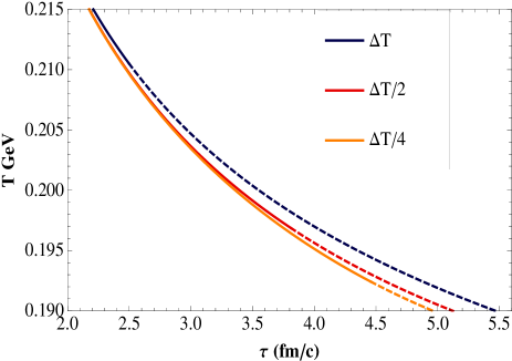
Figure 7: Temperature is plotted as a function of time. With peak value ($a$) of $\zeta/s$ remains same while width ($\Delta T$) varies. Solid line in the curve ends at the time of cavitation, while the dashed lines shows that how system would continue till $T_{c}$ if cavitation is ignored. Figure shows that larger the $\Delta T$ shorter the cavitation time.

In FIGs.6 and 7 we plot $P_{z}$ and $T$ as functions of time for different values of $\Delta T$ while keeping $a$ (=0.901) fixed. It shows that higher value of $\Delta T$ is leading to a shorter cavitation time. For the values of $a~{}\rm{and}~{}\Delta T$ given by equation (19) we find that around $\tau_{c}=2.5~{}fm/c$, $P_{z}$ becomes zero as shown by the curve at the bottom of the FIG.6. In this case cavitation occurs when system temperature is larger than $T_{c}$. This can be seen from the top curve of the in FIG.7. End point of the solid line in the top curve occurs at $T\sim 210~{}MeV$ and $\tau_{c}=2.5~{}fm/c$. Had we ignored the cavitation, system would have taken a time $\tau_{f}=5.5~{}fm/c$ to reach $T_{c}$ which is significantly larger than $\tau_{c}$ as seen from FIG.7. This shows that cavitation occurs rather abruptly without giving any sign in the temperature profile of the system. The hydrodynamic evolution without calculating $P_{z}$ may end up in over estimating the evolution time and subsequent photon production.

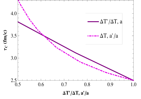
Figure 8: Cavitation time $\tau_{c}$ as a function of different values of height ($a^{\prime}$) and width ($\Delta T^{\prime}$) of $\zeta/s$ curve.

A similar analysis can be carried out by keeping $\Delta T$ fixed ($=T_{c}/14.5$) and varying parameter $a$. We show the cavitation times corresponding to changes in $a$ and $\Delta T$ (denoted by $a^{\prime}$ and $\Delta T^{\prime}$) in FIG.8. The dashed curve in FIG.8 shows $\tau_{c}$ as a function of $a$, while keeping $\Delta T$ fixed. The curve shows that $\tau_{c}$ decreases with with increasing $a$. Solid line shows how $\tau_{c}$ varies while keeping $a$ fixed and changing $\Delta T$.

Thermal Photon Production

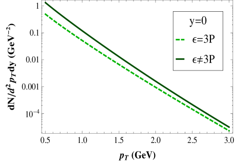
Figure 9: Photon flux as function of transverse momentum for different equation of states. No effect of viscosity included in the hydrodynamical equations.

We have already seen that the calculation of photon production rates require the initial time $\tau_{0}$, final time $\tau_{1}$ and $T(\tau)$. $\tau_{1}$ and $T(\tau)$ are determined from the hydrodynamics. Generally $\tau_{1}$ is taken as the time taken by the system to reach $T_{c}$, i.e.; $\tau_{f}$. But when there is cavitation, we must set $\tau_{1}=\tau_{c}$. Therefor photon productions will be influenced by cavitation, temperature profile and non-ideal EoS near $T_{c}$.

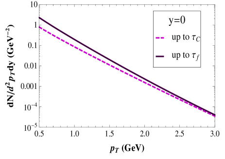
Figure 10: Photon spectrum obtained by considering the effect of cavitation (dashed line). For a comparison we plot the spectrum without incorporating the effect of cavitation (solid line).

FIG. (9) shows the photon production rate calculated using ideal (massless) and non-ideal EoS. The figure shows that non-ideal EoS case can yield significantly larger photon flux as compared to the ideal EoS. At energy $E=1$ GeV, photon flux for the non-ideal EoS is 60$\%$ larger than that of ideal EoS case. This is because the calculation of the photon flux is done by performing time integral over the interval between the initial time $\tau_{0}$ and the final time $\tau_{f}$. $\tau_{0}$ is same for both the system while the $\tau_{f}$ for the case with non-ideal EoS is two times larger than the ideal EoS. Since the non-ideal EoS allows the system to have consistently higher temperature over a longer period as compared to the massless ideal-gas EoS, more photons are produced.

Next we try to observe the effect of cavitation in photon production. We emphasis that rates should only be integrated up to $\tau_{c}$. In FIG.10, photon rates are calculated for the two cases. In the dashed curve the effect of cavitation is taken into account and $\tau_{1}=\tau_{c}=2.5~{}fm/c$. The solid line represent the same case but with the effect of the cavitation is ignored and $\tau_{1}=\tau_{f}=5.5~{}fm/c$. We see from the solid curve that we end up over estimating the photon rates at $p_{\bot}=0.5$ GeV by $\sim$ 200 $\%$ and $p_{\bot}=2$ GeV over estimation is about 50$\%$. So it is clear that information about cavitation time is crucial for correctly estimating thermal photon production rate.

In the FIG.11 we plot photon production rates for various cavitation times obtained by varying $\Delta T$ (with $a=0.901$ is fixed). Here the enhancement in the photon production when $\Delta T$ is reduced to half of its base value is $\sim 75\%$ at $p_{\bot}=0.5$ GeV and $\sim 55\%$ at $p_{\bot}=1$ GeV. A further reduction of the parameter value to $\Delta T/4$ is enhancing the photon production by $\sim 110\%$ at $p_{\bot}=0.5$ GeV and $\sim 80\%$ at $p_{\bot}=1$ GeV. Reduction in $\Delta T$ amounts to increase in the cavitation time, which in turn would increase the time interval over which photon production is calculated. Therefor this increases the photon flux.

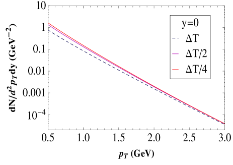
Figure 11: Photon production rates showing the effect of different cavitation time.

IV SUMMARY AND CONCLUSIONS

Thus using the second order relativistic hydrodynamics we have analyzed the role of non-ideal effects near $T_{c}$ arising due to the equation of state, bulk-viscosity and cavitation on the thermal photon production. Since the experiments at RHIC imply extremely small values for $\eta/s$, the shear viscosity play a sub dominant role near $T_{c}$ in the photon production.

We have shown using non-ideal EoS using the recent lattice results that the hydrodynamical expansion gets significantly slow down as compared to the case with the massless EoS. This in turn enhances the flux of hard thermal photons.

Bulk viscosity play a dual role in heavy-ion collisions: On one hand it enhances the time by which the system attains the critical temperature, while on the other hand it can make the hydrodynamical treatment invalid much before it reaches $T_{c}$. We have shown that if the phenomenon of cavitation is ignored one can have erroneous estimates of the photon production. Another result we would like to emphasize is that reduction in cavitation time can lead to significant reduction in the photon production. We hope that this feature may be useful in investigating the signature of cavitation.

References

- (1) J. Kapusta, P. Lichard and D. Seibert, Phys. Rev. D 44, 2774 (1991).
- (2) R. Baier, H. Nakkagawa, and K. Redlich, Z. Phys. C 53, 433 (1992).
- (3) P. V. Ruuskanen, Nucl. Phys. A 544, 169c, (1992).
- (4) M. H. Thoma, Phys. Rev. D 51, 862, (1995).
- (5) C. T. Traxler, H. Vija, and M. H. Thoma, Phys. Lett. B 346, 329 (1995)
- (6) P. Arnold, G. D. Moore and L. G. Yaffe, JHEP 057, 011 (2001); P. Arnold, G. D. Moore and L. G. Yaffe, JHEP 09, 012 (2001).
- (7) J. Alam, S. Sarkar, P. Roy, T. Hatsuda and B. Sinha, Ann. Phys. (NY) 286, 159 (2001).
- (8) T. Peitzmann and M. H. Thoma, Phys. Rept. 364, 175-246 (2002), arXiv: hep-ph/0111114.
- (9) C. Gale and K. L. Haglin, arXiv: hep-ph/0306098v3.
- (10) J. Kapusta and C. Gale, Finite Temperature Field Theory, Cambridge University Press, (2006).
- (11) E. L. Fienberg, Nuovo Cim. A 34, 391 (1976)
- (12) E. V. Shuryak, Phys. Lett. 78, 150 (1978)
- (13) D. K. Srivastava, Eur. Phys. J. C 10, 487-490 (1999)
- (14) F. D. Steffen, and M. H. Thoma, Phys. Lett. B 510, 98-106 (2001)
- (15) D. K. Srivastava, J. Phys. G: Nucl. Part. Phys. 35, 104026, (2008).
- (16) F. M. Liu and K. Werner, J. Phys. G: Nucl. Part. Phys. 36, 035101, (2009).
- (17) J. R. Bhatt and V. Sreekanth, Int. J. Mod. Phys. E 19, 299-306, (2010)
- (18) K. Dusling, arXiv:0903.1764 [hep-th]
- (19) T. Schaefer and D. Teaney, Rept. Prog. Phys. 72, 126001, (2009).
- (20) P. K. Kovtun, D. T. Son and A. O. Starinets, Phys. Rev. Lett. 94, 111601 (2005)
- (21) T. Hirano and M. Gyulassy, Nucl. Phys. A769, 71 (2006).
- (22) K. Adcox et al. [PHENIX Collaboration]; Nucl. Phys. A757, 184 (2005); B. B. Back et al. [PHOBOS Collaboration]; Nucl. Phys. A757, 28 (2005) [arXiv:nucl-ex/0410022]; I. Arsene et al. [BRAHMS Collaboration]; Nucl. Phys. A757, 1 (2005) J. Adams et al. [STAR Collaboration]; Nucl. Phys. A757, 102 (2005) B. Alver et al. [PHOBOS Collaboration], Phys. Rev. Lett. 98, 242302 (2007) B. I. Abelev et al. [STAR Collaboration], Phys. Rev. C 77, 054901 (2008)
- (23) R. Baier and P. Romatschke, Eur. Phys. J. C 51, 677 (2007).
- (24) P. Romatschke and U. Romatschke, Phys. Rev. Lett. 99, 172301 (2007).
- (25) K. Dusling and D. Teaney, Phys. Rev. C 77, 034905 (2008).
- (26) H. Song and U.W. Heinz, Phys. Rev. C 77, 064901 (2008).
- (27) M. Luzum and P. Romatschke, Phys. Rev. C 78, 034915 (2008) [Erratum-ibid. C 79, 039903 (2009)]
- (28) D. Molnar and P. Huovinen, J. Phys. G 35, 104125 (2008)
- (29) H. Song and U. W. Heinz, arXiv:0812.4274 [nucl-th].
- (30) M. Luzum and P. Romatschke, arXiv:0901.4588 [nucl-th].
- (31) S. Weinberg, Gravitation and Cosmology, (John Wiley & Sons, 1972).
- (32) A. Bazavov et al., Phys. Rev. D 80, 014504 (2009)
- (33) H. B. Meyer, Phys. Rev. Lett. 100, 162001 (2008)
- (34) R. J. Fries, B. Müller, and A. Schäffer, Phys. Rev. C 78, 034913 (2008)
- (35) K. Rajagopal, and N. Tripuraneni, JHEP 1003, 018 (2010)
- (36) J. D. Bjorken, Phys. Rev. D 27, 140 (1983).
- (37) D. Teaney, Phys. Rev. C 68, 034913 (2003).
- (38) U. W. Heinz, H. Song, and A. K. Chaudhuri, Phys. Rev. C 73, 034904 (2006).
- (39) A. Muronga, Phys. Rev. C 76, 014909 (2007).
- (40) A. Muronga, Phys. Rev. Lett. 88, 062302 (2002), [Erratum-ibid. 89, 159901 (2002)].
- (41) W. A. Hiscock and L. Lindblom, Phys. Rev. D 31, 725 (1985).
- (42) R. Baier, P. Romatschke, and U. A. Wiedemann, Phys. Rev. C 73, 064903 (2006).
- (43) W. Israel, Ann. Phys. 100, 310 (1976); W. Israel and J. M. Stewart, Ann. Phys. 118, 341 (1979).
- (44) A. Muronga and D. H. Rischke, (2004) arXiv:nucl-th/0407114.
- (45) P. Romatschke, Int. J. Mod. Phys. E 19, 1-53, (2010).
- (46) U. Heinz, arXiv:nucl-th/0512049.
- (47) R. Baier, P. Romatschke, D. T. Son, A. O. Starinets and M. A. Stephanov, JHEP 0804, 100 (2008).
- (48) M. Natsuume and T. Okamura, Phys. Rev. D 77, 066014 (2008).
- (49) S. Bhattacharyya, V. E. Hubeny, S. Minwalla and M. Rangamani, JHEP 0802, 045 (2008)
- (50) F. Karsch, D. Kharzeev, and K. Tuchin, Phys. Lett. B 663, 217 (2008)
- (51) D. Kharzeev and K. Tuchin, JHEP 0809, 093 (2008)
- (52) P. Aurenche, F. Gelis, H. Zaraket, and R. Kobes, Phys. Rev. D 58, 085003 (1998)
- (53) F. Karsch, Z. Phys. C 38, 147 (1988)
- (54) C. T. Traxler and M. H. Thoma, Phys. Rev. C 53, 1348 (1996)