MODELS AND SIGNATURES OF EXTRA DIMENSIONS AT THE LHC

Models for extra dimensions and some of the most promising ensuing signals for experimental discovery at the LHC are briefly reviewed. The emphasis will be put on the production of Kaluza Klein states from both flat and warped extra-dimensions models.

1 Introduction

One of the first motivation for the recent renewed interest for extra dimensions (since the early years of the 20th century, back in the G.  Nordström $\!{}^{{\bf?}}$, T. Kaluza $\!{}^{{\bf?}}$, O. Klein $\!{}^{{\bf?}}$ A. Einstein and P. Bergmann $\!{}^{{\bf?}}$ time where they were first discussed from the physics point of view  and since some further developments from the 50’s to the 70’s) comes from the possibility they have to address the hierarchy problem of the standard model of particle physics. In the course of their development, it quickly appears that they can also address some other issues such as symmetry breaking, provide some understanding for masses and mixing of the Standard Model fermions, allow for TeV scale unification without supersymmetry and provide dark matter candidates. There are also strong motivations for extra dimensions from more fundamental underlying candidate theories such as for example string theories that will not be discussed in the following since it would bring this short review too far out of scope.

There are many possible approaches for extra dimensions models connected to basic questions such as: how many extra dimensions can there be ? Which geometry can they have ? How large can they be, with which consequences for the phenomenology ? Which fields are sitting where ?

There are two kinds of possible geometries for extra dimensions. One is called factorizable or flat where one can have in principle any number of extra dimensions i.e. 3 space dimensions + 1 time dimension + $D-4$ extra-dimensions, with a metric written in the so called usual way $ds^{2}=g_{\mu\nu}dx^{\mu}dx^{\nu}$ ($\mu,\nu=0,1,2,3...D$). The other one is called non factorizable or warped and is characterized by the presence of a warp factor $a(y)$, depending on usually only one extra-dimension $y$, put in front of the 4 dimensional metric (often identified with the Minkowki metric $\eta_{\mu\nu}$) $ds^{2}=a(y)(\eta_{\mu\nu}dx^{\mu}dx^{\nu})+dy^{2}$ (where here $\mu,\nu=0,1,2,3$).

Extra dimensions have not yet been seen experimentally so if they exist they must be small (for flat geometries) i.e. compact. Compactifying extra dimensions leads to some periodicity conditions on fields so that one can Fourier expand them:

$$\phi(x_{\mu},y)=\sum_{k=-\infty}^{+\infty}{\phi^{(k)}(x_{\mu})}e^{{{iky}\over{R}}}$$ (1)

and separate the 4 dimensional component which gives rise to the so called Kaluza-Klein (KK) modes or states or excitations ${\phi^{(k)}(x_{\mu})}$. The number of KK states is infinite. They are massive and the mass of the $k^{th}$ mode is given by the inverse compactification size/radius $R$:

$$m^{2}_{k}=m^{2}_{o}+{{k^{2}}\over{R^{2}}}.$$ (2)

Answering the question which field is sitting where leads to an immense variety of possible approaches for extra dimensions. One of the first and simplest approach is the so called ADD model $\!{}^{{\bf?}}$ where only gravity propagates in the full D dimensional spacetime with flat geometry and with n compactified extra space dimensions which will be called the bulk . The compactified extra dimensions can be quite large as we will see later on. The Standard Model fields are confined on a 4 dimensional sub-spacetime which will be called brane. The so called $TeV^{-1}$ models are models where one can have one or more small compactified extra dimensions with flat geometries with sizes of the order of the inverse of the TeV scale i.e. $O(10^{-19})\,m$, where the Standard Model gauge bosons can propagate  $\!{}^{{\bf?}}$. This whole setup can be embedded in a larger space where gravity propagates. The fermions of the Standard Model are still confined on a 4 dimensional sub-spacetime. Universal extra-dimension (UED) models $\!{}^{{\bf?}}$ are models with flat geometry where Standard Model gauge bosons as well as fermions can propagate in the bulk with one (or more recently two) extra dimension. An important set-up is the so called RS setup $\!{}^{{\bf?}}$ which is a setup where gravity only propagates in a 5 dimensional warped bulk with one compactified extra dimensions and with two 4 dimensional branes. The Standard Model fields are confined on one brane i.e. the infrared or TeV brane, is at the TeV scale while the other brane, the Planck brane, is at the Planck scale. One can further extend the previous minimal RS setup by putting a scalar field in the warped bulk which will allow to stabilize the interbrane distance $\!{}^{{\bf?}}$. In the following, this approach will be referred to as the stabilized RS approach. One can further extend the previous setup by putting Standard Model gauge boson as well Standard Model fermions in the warped bulk (with the Higgs boson field being localized near the TeV brane) which is presently giving rise to a huge activity and, in the following, will be referred to as the bulk RS approach.

Anticipating a bit on the following, extra dimensions model building becomes very challenging especially in view of the present electroweak precision measurements and the experimental constraints from flavor physics.

The outline of this short overview naturally follows the above discussion and will be divided into two main parts. The first part will focus on the flat extra dimension models with the ADD, $TeV^{-1}$ and UED models. The second part will be devoted to the warped extra dimension models with minimal RS, stabilized RS and Bulk RS models.

Every possible models and signatures at the LHC will not be touched upon in this short overview because there are way too many for the size of this mini-eview but instead some examples will be picked up to illustrate each topic mentioned in the outline.

Higgsless models is discussed in $\!{}^{{\bf?}}$. Black holes, string states, supersymmetric extra dimensions models as well as models from intersecting branes (including intersecting branes at angle) will not be discussed in this short overview.

2 Flat compactified extra dimensions models

2.1 ADD models

As already mentioned, the ADD model is an approach where only gravity propagates in a bulk of $4+n$ dimensions with $n$ compactified extra dimensions. The Standard Model fields are confined on a 4 dimensional brane. This model addresses the hierarchy problem since one can relate the ordinary 4 dimensional Planck scale $M^{2}_{Pl(4)}$ to a fundamental TeV scale via an extra-dimension volume factor $R^{n}$:

$$M^{2}_{Pl(4)}=M^{n+2}_{Pl(4+n)}R^{n}$$ (3)

where $R$ stands for the size of the $n$ compact extra dimensions. For a fundamental scale $M_{D}=M_{Pl(4+n)}$ of the order of 1 TeV, very large extra dimensions can be expected. For example, in the case of one extra dimension, the size of the extra dimension can be of the order of the size of the solar system. Having in mind that the ADD approach also predicts important deviations from the Newton law of classical gravitation, one can see that the one extra dimension case is already ruled out experimentally since no subsequent effect of have been observed at the level of the solar system. In the case of 2 or more extra dimensions the size can be of the order of the millimeter or nanometer. This scenario does not contradict submillimetric gravity measurements $\!{}^{{\bf?}}$ especially if the effects of the shape of the compactifying space is taken into account, even in the simplest case of toroïdal compactifications $\!{}^{{\bf?}}$.

In addition to submillimetric gravity measurements one can also constrain the ADD scenario from various areas such as astrophysics and cosmology as well collider physics and explore its phenomenology. In the following the focus will be put on collider physics $\!{}^{{\bf?}}$ and more specifically the LHC. At colliders the production of KK graviton states provides the handle to sign the existence of compact extra dimensions. One can have so called direct searches where KK gravitons are present in the final state. In the ADD approach the KK graviton states are close to each other in mass namely with mass differences down to a fraction of electron volt:

$$\Delta m\sim({M_{D}\over TeV})^{{n+2}\over 2}10^{{12n-31\over n}}$$ (4)

so that they form a quasi continuum of states which compensates the smallness of their individual coupling to Standard Model field which is of the order of the inverse of the usual 4 dimensional Planck mass $1/M_{Pl(4)}$. At the LHC KK gravitons can be produced in association with a jet from a quark or a gluon, with a photon ($\gamma$) or a Z boson thus giving rise to jet + missing energy, $\gamma$ + missing energy or Z + missing energy signature respectively (where the missing energy component is due to the escaping KK graviton). The production cross sections are sizeable and directly related to the number of extra dimensions $n$ and to the scale $M_{D}$. One can also have indirect searches where no KK graviton states are present in the final states. Thus one has to look for deviations in fermion or boson pair production with respect to the prediction of the Standard Model. In contrast to the direct searches, the cross sections are not directly related to the fundamental scale. For 2 and more extra dimensions the cross sections diverge and, in the context of field theory , the introduction of a cut-off is required. However this cut-off is related to the fundamental scale only through an arbitray factor which is usually taken equal to 1. Current collider constraints from HERA, LEP and Tevatron on scales are of the order of $1.6-2.1$ TeV for 2 extra dimensions.

At the LHC one can look at mono-jet events as done for example by the CMS experiment $\!{}^{{\bf?}}$. One can look for an excess of events over the background in observables such as the vectorial sum of jets $p_{T}$ after a simple set of cuts. Either exclusions above the current constraints or discovery can be achieved with relatively low luminosities i.e. O(100) pb^-1, as shown in Fig. 1 from $\!{}^{{\bf?}}$. Similar conclusions can be reached for indirect searches for example in the $\gamma\gamma$ channel as shown in $\!{}^{{\bf?}}$.

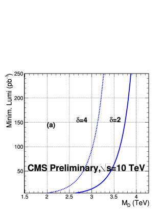
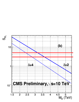
Figure 1: (a): exclusion at 95% C.L. showing the minimum luminosity to exclude a given value of $M_{D}$. (b): discovery potential as a function of $M_{D}$ for various number of extra dimensions $\delta$ after 200 pb^-1 of integrated luminosity. The horizontal lines correspond to $3\sigma$ and $5\sigma$ significance level. Both plots assume ${\sqrt{s}}=$10 TeV.

2.2 $TeV^{-1}$ Models

As already mentioned TeV^-1 models are models where the Standard Model gauge bosons can propagate in a bulk with small compactified extra-dimensions of size of the order of TeV^-1. For simplicity we can here consider models with only one extra dimension. In fact it has been shown that the 5 dimensional effective gauge couplings are finite while for more than one extra dimension they become divergent . The standard model fermions are confined on a 4 dimensional brane and the KK 0^th mode of the gauge bosons are identified with the 4 dimensional Standard Model gauge bosons. A global fit including not only electroweak precision measurements but also high energy data from LEP, HERA and the Tevatron Run 1 allows to set a lower limit of 6.8 TeV on the KK gauge bosons masses $\!{}^{{\bf?}}$. Direct searches at present colliders set lower limits of the order of 1 TeV. If kinematically allowed, KK gauge bosons can be resonantly produced at the LHC and one can look for a resonance decaying into fermions pairs. Otherwise one has to rely on indirect effects and look for deviations in fermion pair production cross sections measurements and asymmetries with respect to the predictions of the Standard Model. For example the study of the search for resonances has been done in a quite generic way at the LHC for both Z’ and W’ types of gauge bosons. Depending on particular models and detector performances (lepton identification, missing energy resolution) one can achieve a $5\sigma$ discovery from 1 TeV with O(10) pb^-1 of well understood data up to 3 TeV where much more integrated luminosities are required namely in the O(10-100) fb^-1 region as shown by the ATLAS collaboration $\!{}^{{\bf?}}$.

2.3 Universal extra dimension (UED) models

UED models are models where all Standard Model fields propagate in the bulk (gravity is not included). The minimal versions of such models are 5 dimensional models with one extra compact dimension. The KK 0^th modes are identified with the 4 dimensional Standard Model particles. The non-zero KK modes are massive and loop corrections involving bulk fields lead to non degenerate mass spectra $\!{}^{{\bf?},{\bf?}}$. The electroweak precision measurements set constraints on the typical mass scale $M$ of this UED scenario $\!{}^{{\bf?}}$ i.e. $M>300$ GeV. These constraints increase up to $M>700$ GeV when taking into account two-loop standard model contributions as well as LEP2 analyses $\!{}^{{\bf?}}$. Momentum conservation considerations in the bulk lead to the conservation of a number call KK-parity which in turn lead to a phenomenology resembling to the phenomenology of supersymmetry with conserved R-parity. Namely UED KK states are pair produced, a UED KK state decays into a UED KK state and a particle of the Standard Model i.e. cascade decays can occur, and finally there exists a lightest KK particle, the LKP, which is stable and which can escape a detector at colliders thus being a source of missing energy. The LKP provides a dark matter candidate which can be either the first KK mode of a photon $\gamma_{1}$ or the first KK mode of a neutrino $\nu_{1}$ $\!{}^{{\bf?}}$. At the LHC the pair production of the lightest coloured KK states have the largest production cross-sections $\!{}^{{\bf?}}$. The production of UED KK states, after cascade decays, can then lead to signatures such as multileptons and missing transverse energy or multi leptons , multijets and missing transverse energy or multijets and missing transverse energy i.e. similar to supersymmetry signatures. As shown for example in $\!{}^{{\bf?}}$, in the 4 leptons and missing transverse energy channels, one can expect a $5\sigma$ discovery (at ${\sqrt{s}}=14$ TeV) above the current constraints with more than O(1) fb^-1 of integrated luminosity. It would also be desirable to distinguish minimal UED signatures from supersymmetry signatures. In order to achieve this goal, one of the best way would be to search for the second level of KK states, namely start to look for the KK tower structure. At similar masses the cross sections of UED processes are greater than the cross section of supersymmetric processes (because both left and right handed SU(2) doublet KK fermions are present in UED while one has only left handed SU(2) squarks doublet, one integrates different angular distribution i.e. $(1+\cos^{2}\theta)$ for fermions versus ($1-\cos^{2}\theta$) for scalars and for production close to threshold one has different cross section threshold suppression i.e. $\beta$ for fermions versus $\beta^{3}$ for scalars). Level 2 KK quarks can be directly pair produced (or produced in association with KK gluons). However cross section times branching ratios for multi-leptons and missing transverse energy channels, for example, are still challengingly small and there are challengingly small statistics to distinguish from level 1 modes. Alternatively the search for level 2 KK gauge boson $V_{2}$ offers good prospect $\!{}^{{\bf?}}$ in particular when one includes the possibility of single KK gauge boson production via KK number violation interactions (but still with KK parity conservation) i.e. looking for processes such as $pp\rightarrow V_{2}\rightarrow f_{0}{\bar{f}}_{0}$ where $f_{0}$ stands for fermion a 0^th KK level namely a fermion of the Standard Model. One striking signature would be a double peak structure of $\gamma_{2}$ and $Z_{2}$ in dilepton invariant masses as shown in Fig. 2 with near mass degeneracy further corrobating the UED interpretation. Preliminary studies $\!{}^{{\bf?}}$ show that one should be able to explore the O(0.6-1) TeV mass range using from O(1) fb^-1 up to O(100) fb^-1 of integrated luminosity (at ${\sqrt{s}}=14$ TeV).

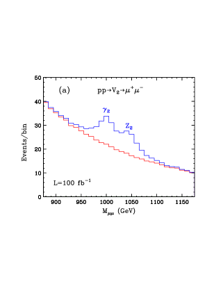
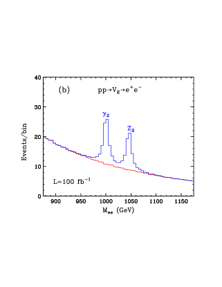
Figure 2: The $\gamma_{2}-Z_{2}$ diresonance structure in UED (see text) with with $R^{-1}=500$ GeV for the dimuons (a) and dielectron channel (b) at the LHC with with 100 fb^-1 of integrated luminosity (at ${\sqrt{s}}=14$ TeV) .

3 Warped extra dimension models

3.1 Minimal Randall Sundrum (RS) models

As mentioned in the introduction, Randall and Sundrum (RS) $\!{}^{{\bf?}}$ proposed a phenomenological model with two 4 dimensional branes in a 5 dimensional space-time with a warped geometry where gravity propagates (minimal RS). One can write the metric as $ds^{2}=e^{-2kr_{c}\phi}\eta_{\mu\nu}dx^{\mu}dx^{\nu}+r_{c}d\phi^{2}$ with a compact 5^th dimension where $\phi$ sits in $[0,\pi]$ and with the warp factor $e^{-2kr_{c}\phi}$ where $k$ is a dimensionful parameter of the order of the 5 dimensional Planck scale $M_{5}$. In contrast to the ADD relation (eq. 3), the 4 dimensional Planck scale in the RS approach is given by:

$${M}^{2}_{Pl(4)}={M^{3}_{5}\over k}[1-e^{-2kr_{c}\pi}]$$ (5)

so that $k$, $M_{5}$ and ${M}^{2}_{Pl(4)}$ have comparable magnitude when the warp factor is small. The warp factor allows to generate a low energy scale on one brane (TeV brane), from a high energy scale, typically the Planck scale, on the other brane (the Planck brane). In particular a $\Lambda_{\pi}=M_{pl(4)}e^{-kr_{c}\pi}$=1 TeV energy scale can be generated from the 4 dimensional Planck scale if $kr_{c}\sim 12$ ($r_{c}=10^{-32}$ m) thus allowing to solve the hierarchy problem. In contrast to the ADD approach the graviton field expansion into KK modes in the RS approach is given by a linear combination of Bessel functions. In consequence the masses of the KK gravitons are not regularly spaced but are given by $m_{n}=x_{n}ke^{-k\pi r_{c}}$ where $x_{n}$ are the roots of Bessel functions. Furthermore the order of magnitude of the mass of the first KK graviton mode is O(1) TeV. The Standard Model fields are localized on the TeV brane. The coupling of the 0^th mode graviton to standard model fields is inversely proportional to the 4 dimensional Planck mass and is thus suppressed. Nevertheless the coupling of the non zero KK graviton modes is inversely proportional to $e^{-k\pi r_{c}}M_{Pl}$ namely the 4 dimensional Planck mass multiplied by the warp factor. i.e. the coupling of the non zero KK graviton modes to the standard model fields is enhanced by the warp factor $e^{k\pi r_{c}}$. KK graviton modes are resonantly produced at colliders if they are kinematically accessible. Once they are produced they decay predominantly into two jets $\!{}^{{\bf?}}$ and then into other decay channels such as $W^{+}W^{-}$, $ZZ$, $l^{+}l^{-}$, $t\bar{t}$ and $hh$. Although leptonic decay channels are not dominant they offer a clear signature in particular at the LHC. The phenomenomlogy of this minimal RS approach can be described by two parameters namely the mass $M_{1}$ of the first KK graviton mode and a parameter $c=M_{1}/(x_{1}\Lambda_{\pi})$ where typically $0.01<c<0.1$. Searches for the KK graviton have been performed at the Tevatron and constraints have been set $\!{}^{{\bf?}}$. By looking for a resonance decaying into electron pairs it has also been shown that the LHC should be able to cover the whole region of interest with less than 100 fb^-1 at ${\sqrt{s}}=14$ TeV as shown in $\!{}^{{\bf?}}$ and $\!{}^{{\bf?}}$. It has also been shown that one should be able to distinguish between spin 1 and spin 2 resonances by using angular distribution in the lepton lepton center of mass frame $\!{}^{{\bf?}}$.

3.2 Stabilized RS

There are gravitational fluctuations around the RS metric which contain a massless scalar mode called the radion. The presence of this scalar field in the bulk with interactions localized on the branes allows to stabilize the value of $r_{c}$ i.e. the interbrane distance $\!{}^{{\bf?}}$. In order to recover ordinary 4 dimensional Einstein gravity the radion must be massive and, for this stabilized RS model to still solve the hierarchy problem, the radion should be lighter than the KK graviton. It turns out out that the radion is likely to be the lightest state from the RS models. The radion couple to Standard Model fields via the trace of the energy-momentum tensor and can have direct coupling to gluon and photon. The phenomenology of the radion resembles to the phenomenology of the Higgs boson for both production and decay except for this direct coupling to gluon which allows to enhance the production with respect to the Higgs boson and modify the light radion decay $\!{}^{{\bf?}}$. The radion predominantly decays into a gluon pair at low mass or W pair above the WW mass threshold. Besides, there also is, in addition, possible mixing between the Standard Model Higgs boson and the radion which allows to consider new physical mass eigenstates. The decay branching ratios of these new eigenstates are different from those of the Standard Model Higgs boson. Depending on the value of the coupling which is responsible of the Higgs boson-radion mixing the difference can be sizeable i.e. up to a factor 50 for the $W^{+}W^{-}$ et $ZZ$ decays. This mixing can also lead to non negligible branching ratios for invisibly decaying Standard Model Higgs boson. This analysis has been confirmed in a more fundamental context involving type I string theory $\!{}^{{\bf?}}$. The Opal collaboration $\!{}^{{\bf?}}$ performed a search for the radion via existing searches of the Higgs boson. No evidence for the radion has been found and the Opal collaboration derived constraints on the parameters of the stabilized RS model (see $\!{}^{{\bf?}}$) for various scenario of Higgs-radion mixing. Pure radion effects (i.e. without the above mentioned mixing) on precision electroweak observables have been shown to be small $\!{}^{{\bf?}}$. It is possible to use the Standard Model Higgs boson searches to search for the radion $\!{}^{{\bf?}}$ as shown in Fig. 3 from M. Toharia $\!{}^{{\bf?}}$ where the explorable domain in the radion coupling and mass plane ($\Lambda_{\phi}={\sqrt{6}}\Lambda_{\pi}$,$m_{\phi}$) in a model where all Standard Model fields are in the RS bulk $\!{}^{{\bf?}}$ (anticipating a bit on the next section).

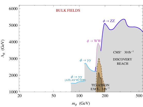
Figure 3: Discovery reach for the radion at the LHC from Higgs boson searches from ATLAS and CMS (see text).

3.3 Bulk RS models

Shortly after the development of the minimal and stabilized RS models, it has been realized that in order to solve the hierarchy problem of the Standard Model only the Standard Model Higgs has to be localized near the TeV brane thus giving rise to the bulk RS models $\!{}^{{\bf?}}$. In the bulk RS models, Standard Model fermions and gauge bosons are allowed to propagate in the RS bulk and the 4 dimensional Standard Model particles correspond to the 0^th mode of the 5 dimensional fields. The bulk profile of the Standard Model fermion wave function depends on its five dimensional mass parameter. The Yukawa coupling of Standard Model fermions depend on the overlap of their wave function with the wave function of the Higgs boson. In other words the masses and Yukawa couplings of the Standard Model fermions depend on the bulk profile of the corresponding 5 dimensional fields. Thus bulk RS models allow to understand the Standard Model Yukawa coupling hierarchies and allow to suppress dangerous FCNC from higher dimensional couplings. One can choose to localize the 1st and 2nd generation fermions near the Planck brane where their wave functions have small overlaps between with the wave function of the Higgs boson (localized near the TeV brane). One can also choose also to localize the top and bottom quarks near the TeV brane with a bigger overlap of their wave functions with the wave function of the Higgs boson giving rise to bigger Yukawa coupling. Electroweak precision data (including $Z\rightarrow b_{L}{\bar{b}}_{L}$) and data from flavor physics (K and B physics, CP violation, rare decays) are very constraining for the bulk RS models $\!{}^{{\bf?}}$ $\!{}^{{\bf?}}$. With the help of additionnal symmetries in the RS bulk such as custodial isospin symmetries sufficient to suppress excessive contributions to the T parameter (and flavour symmetries) one can lower the lower limits/constraints on KK masses namely O(3 TeV) for KK gauge bosons, O(2-4 TeV) for KK graviton and O(1-2 TeV) for fermions excitations. Without fermions in the bulk (i.e. having only gauge bosons in the bulk) and without custodial symmetries the lower limits on KK graviton and KK gauge bosons would have been in the O(30-40 TeV) region i.e. well beyond the reach of the LHC. Constraints from flavour physics are still striking hard any realistic model building attempt and a lot of effort is being put in RS flavor models developments $\!{}^{{\bf?}}$ which are beyond the scope of this short overview.

There are many possible signatures for bulk RS models at the LHC $\!{}^{{\bf?}}$. KK gravitons (1st mode $G^{1}$) localized near the TeV brane can be resonantly and produced dominantly through the process $gg\rightarrow G^{(1)}$ for which the gluon profile in the bulk is supposed to be flat. The 1^st generation fermions being localized near the Planck brane they have small wave functions overlap with the KK graviton and hence the KK graviton coupling to u and d quarks is suppressed. At the LHC the production of KK gravitons then occurs dominantly via gluons. KK gravitons have decays which differ from the decays of the minimal RS model i.e. KK gravitons decay predominantly into $t\bar{t}$, since the 3^rd quark generation fermions is also supposed to be localized near the TeV brane, and into $WW$ and $ZZ$.

KK gluons ($g^{(1)}$) and KK gauge bosons ($Z^{(1)},W^{(1)}$) can also be resonantly produced with $g^{(1)}\rightarrow t\bar{t}$, $Z^{(1)}\rightarrow WW$ and $W^{(1)}\rightarrow Wh$ decays. Finally KK fermions can be pair produced via for example $pp\rightarrow g+g^{(1)}\rightarrow t^{(1)}{\bar{t}}^{(1)}$.

Assuming for example a 10% top identification efficiency, it has been shown that a 5 $\sigma$ reach (i.e. here in terms of $S/{\sqrt{B}}$ where S stands for the $gg\rightarrow G^{(1)}\rightarrow t\bar{t}$ signal and B for the background from the Standard Model top quark pair production) can be achieved at the LHC (with ${\sqrt{s}}=14$ TeV) for top quarks localized very near the TeV brane and for not too heavy KK gravitons i.e. in the O(1-2 TeV) mass range.

The top quarks from the KK graviton decay are expected to be boosted. Improvements in the KK graviton mass reach are expected with the use of boosted top jet algorithms $\!{}^{{\bf?}}$ in order to improve the top tagging and identification efficiencies. For example such algorithms have been used to search for KK gluons $\!{}^{{\bf?}}$ in all hadronic channels i.e. $pp\rightarrow g^{(1)}\rightarrow t{\bar{t}}\rightarrow b{\bar{b}}jjjj$. It has been shown that a typical 40 % efficiency can be obtained for jet $p_{T}$ greater than 700 GeV for a fake tag rate below 6 % and that a $5\sigma$ discovery can be made for cross sections of 43.6, 4, 1.6 and 1.3 pb respectively, this with 100 pb^-1 of integrated luminosity at ${\sqrt{s}}=$ 10 TeV.

4 conclusion

There is a wide spectrum of possible models and signatures of extra-dimensions which can be explored at the LHC. There are strong constraints from electroweak precision data and data flavor physics which are very challenging for realistic model building. Some examples of non-resonant KK states searches with mono jets as well searches for KK resonances in dileptons, di-boson and top quark pairs as well as the use of Higgs boson searches have been discussed. Signal discovery can be achieved with relatively low integrated luminosities considering optimistic model parameters and not too high KK states masses. However to establish that the discovered signals are actually coming from extra dimensions and further dedicated studies may need a LHC running at the highest possible center of mass energy and higher integrated luminosities.

References

References

- [1] G. Nordström, Phys. Z. 15 (1914) 504.
- [2] T. Kaluza, Sitzungsber. Preuss. Akad. Wiss. Berlin, Math. Phys. K1 (1921) 966.
- [3] O. Klein, Z. Phys. 37 (1926) 895.
- [4] A. Einstein and P. Bergmann, Ann. Math. 39 (1938) 683.
- [5] N. Arkani-Hamed, S. Dimopoulos, G. Dvali, Phys. Lett. B 429, 263 (1998) and Phys. Rev. D 59, 086004 (1999), I. Antoniadis, N. Arkani-Hamed, S. Dimopoulos, G. Dvali, Phys. Lett. B 436, 257 (1998).
- [6] D. Cremades, L. E. Ibanez, F. Marchesano, Nucl. Phys. B 643, 93 (2002); C. Kokorelis, Nucl. Phys. B 677, 115 (2004).
- [7] I. Antoniadis, Phys. Lett. B 246, 377 (1990), I. Antoniadis, K. Benakli, M. Quiros, Phys. Lett. B 331, 313 (1994) and Phys. Lett. B 460, 176 (1999), K. R. Dienes, E. Dudas, T. Gherghetta, Phys. Lett. B 436, 55 (1998) and Nucl. Phys. B 537, 47 (1999), T. G. Rizzo, J. D. Wells, Phys. Rev. D 61, 016007 (2000).
- [8] T. Appelquist, H. Cheng, B. Dobrescu, Phys. Rev. D 64, 035002 ()2001.
- [9] L. Randall, R. Sundrum, Phys. Rev. Lett. 83, 3370 (1999).
- [10] W. D. Goldberger, M. B. Wise, Phys. Rev. Lett. 83, 4922 (1999), Phys. Rev. D 60, 107505 (1999) and PLB 475, 275 (2000).
- [11] J. Terning these proceedings.
- [12] D. J. Kapner et al, Phys. Rev. Lett. 98, 0211101 (2007).
- [13] K. R. Dienes, A. Mafi, Phys. Rev. Lett. 88, 111602 (2002), Phys. Rev. Lett. 89, 171602 (2002).
- [14] T. Han, J. D. Lykken, R. J. Zhang, Phys. Rev. D 59, 105006 (1999); J. L. Hewett, Phys. Rev. Lett. 82, 4765 (1999); G. F. Giudice, R. Rattazzi and J. D. Wells, Nucl. Phys. B 544, 3 (1999); E. A. Mirabelli, M. Perelstein and M. E. Peskin, Phys. Rev. Lett. 82, 2236 (1999).
- [15] CMS collaboration, CMS PAS EXO-09-013.
- [16] CMS collaboration, CMS PAS EXO-09-004.
- [17] K. M. Cheung, G. Landsberg, Phys. Rev. D 65, 076003 ()2002.
- [18] ATLAS Collaboration, arXiv:0901.0512 see also, CMS Collaboration, CMS PAS EXO-08-004 and CMS PAS EXO-09-006.
- [19] H. C. Cheng, K.T. Matchev and M. Schmaltz, Phys. Rev. D 66, 036005 (2002).
- [20] H. C. Cheng, K.T. Matchev and M. Schmaltz, Phys. Rev. D 66, 056006 (2002).
- [21] T. Flacke, D. Hooper and J. March-Russel, Phys. Rev. D 73, 095002 (2006) and Erratum-ibid.D74, 019902 (2006).
- [22] G. Servant and T. M. P. Tait, Nucl. Phys. B 650, 391 (2003); G. Servant and T. M. P. Tait, New. J. Phys. 4,99 (2002); G. Bertone, G. Servant and G. Sigl, Phys. Rev. D 68, 044008 (2003); D. Hooper and G. Servant, Astropart. Phys. 24, 231 (2005); A. Barrau, P. Salati, G. Servant, F. Donato, J. Grain, D. Maurin and R. Taillet, Phys. Rev. D 72, 063507 (2005); M. Kakizaki, S. Matsumoto, Y. Sato and M. Senami, Nucl. Phys. B 375, 84 (2006).
- [23] T. G. Rizzo, Phys. Rev. D 64, 095010 (2001).
- [24] M. Gigg, P. Ribeiro, arXiv:0802.3715.
- [25] A. Datta, K. Kong, K. T. Matchev, Phys. Rev. D 72, 096006 (2005) and Erratum-ibid. D72,119901 (2005).
- [26] H. Davoudiasl, J. L. Hewett and T. G. Rizzo, Phys. Rev. D 63, 075004 (2001).
- [27] J. Hays, these proceedings.
- [28] ATLAS collaboration, arXiv:0901.0512.
- [29] C. Collard and M. C. Collard, Eur. Phys. J. C 40N5, 15 (2000), see also CMS Collaboration CMS PAS EXO-09-009.
- [30] B. C. Allanach, K. Odagiri, M. A. Parker, B. R. Webber, JHEP 09, 019 (2000).
- [31] U. Mahanta, S. Rakshit, Phys. Lett. B 480, 176 (2000); U. Mahanta, A. Datta, Phys. Lett. B 483, 196 (2000); S. Bae, P. Ko, H. S. Lee, J. Lee, Phys. Lett. B 487, 299 (2000); U. Mahanta, Phys. Rev. D 63, 076006 (2001); K. M. Cheung, Phys. Rev. D 63, 056007 (2001); C. Csaki, M. L. Graesser, G. D. Kribs Phys. Rev. D 63, 065002 (2001); G. F. Giudice, R. Rattazzi, J. D. Wells, Nucl. Phys. B 595, 250 (2001); T. Han, G. D. Kribs, B. Mac Elrath, Phys. Rev. D 64, 076003 (2001); S. Bae, H. S. Lee, Phys. Lett. B 506, 147 (2001); M. Chaichian, A. Datta, K. Huitu, Z. Yu, Phys. Lett. B 524, 161 (2002); P. Das, U. Mahanta, Phys. Lett. B 529, 253 (2002); G. Azuelos, D. Cavalli, H. Przysiezniak, L. Vacavant, Eur. Phys. J. Direct C4, 16 (2002); A. Gupta, N. Mahajan Phys. Rev. D 65, 056003 (2002); J. L. Hewett, T. G. Rizzo, JHEP 08, 028 (2003); M. Battaglia, S. De Curtis, A. De Roeck, D. Dominici, J. F. Gunion, Phys. Lett. B 568, 92 (2003); P. Das, U. Mahanta, Mod. Phys. Lett. A19, 1855 (2004); K. M. Cheung, C. S. Kim, J. Song, Phys. Rev. D 69, 075011 (2004); P. Das, Phys. Rev. D 72, 055009 (2005).
- [32] OPAL collaboration (G. Abbiendi et al), Phys. Lett. B 609, 20 (2005).
- [33] I. Antoniadis, R. Sturani, Nucl. Phys. B 631, 66 (2002).
- [34] J. F. Gunion, M. Toharia, J. D. Wells, Phys. Lett. B 585, 295 (2004).
- [35] P. Nath et al, Nucl. Phys. Proc. Suppl. 200-202, 185 (2010), arXiv:1001,2693.
- [36] M. Toharia, AIP Conf. Proc. 1200, 627 (2010), arXiv:0910.3624.
- [37] T. G. Rizzo, JHEP 06, 056 (2002); D. Dominici, B. Grzadkowski, J. F. Gunion, M. Toharia, Nucl. Phys. B 671, 243 (2003); C. Csaki, J. Hubisz, S. J. Lee Phys. Rev. D 76, 125005 (2007); M. Toharia, Phys. Rev. D 79, 015009 (2009); A. Azatov, M. Toharia, L. Zhu, Phys. Rev. D 80, 031701 (2009); A. Azatov, M. Toharia, L. Zhu, Phys. Rev. D 80, 035016 (2009).
- [38] H. Davoudiasl, J. L. Hewett, T. G. Rizzo, Phys. Lett. B 473, 43 (2000); Y. Grossman, M. Neubert, Phys. Lett. B 474, 361 (2000); A. Pomarol, Phys. Lett. B 486, (1)532000; S. Chang, J. Hisano, H. Nakano, N. Okada and M. Yamaguchi, Phys. Rev. D 62, 084025 (2000); L. Randall, M. D. Schwartz, JHEP 11, 003 (2001); S. J. Huber, Q. Shafi, Phys. Rev. D 63, 045010 (2001), Phys. Lett. B 498, 256 (2001); A. Gupta, N. Mahajan, Phys. Rev. D 65, 056003 (2002); L. Randall, M. D. Schwartz, Phys. Rev. Lett. 88, 081801 (2002); C. Csaki, J. Erlich, J. Terning, Phys. Rev. D 66, 064021 (2002); J. L. Hewett, F .J. Petriello, T. G. Rizzo, JHEP 09, 030 (2002); K. Agashe, A. Delgado, M. J. May, R. Sundrum, JHEP 08, 050 (2003); M. Carena, E. Ponton, T. M. P. Tait, C. E. M. Wagner, Phys. Rev. D 67, 096006 (2003); M. Carena, A. Delgado, E. Ponton, T. M. P. Tait, C. E. M. Wagner, Phys. Rev. D 68, 035010 (2003), Phys. Rev. D 71, 015010 (2005); K. Agashe, G. Perez, A. Soni, Phys. Rev. D 71, 016002 (2005); M. Carena, E. Ponton, J. Santiago, C. E. M. Wagner, Nucl. Phys. B 759, 202 (2006); A. D. Medina, N. R. Shah, C. E. M. Wagner, Phys. Rev. D 76, 095010 (2007); K. Agashe, T. Okui, R. Sundrum, Phys. Rev. Lett. 101801, 2009 (.)
- [39] J. Huber, Nucl. Phys. B 666, 269 (2003); G. Burdman, Phys. Rev. D 66, 076003 (2002), Phys. Lett. B 590, 86 (2004), K. Agashe, G. Perez, A. Soni, Phys. Rev. Lett. 93, 201804 (2004), Phys. Rev. D71 016002, 2005 (;) K. Agashe, R. Contino, L. Da Rold, A. Pomarol, Phys. Lett. B 641, 62 (2006); G. Moreau, J. I. Silva-Marcos, JHEP 03, 090 (2006); K. Agashe, R. Contino, Nucl. Phys. B 742, 59 (2006); M. Carena, E. Ponton, J. Santiago, C. E. M. Wagner, Phys. Rev. D 76, 035006 (2007); A. Delgado, A. Falkowski, JHEP 05, 097 (2007), A. Djouadi, G. Moreau, F. Richard, Nucl. Phys. B 773, 43 (2008); G. Cacciapaglia, C. Csaki, J. Galloway, G. Marandella, J. Terning, A. Weiler, JHEP 04, 006 (2008); S. Casagrande, F. Goertz, U. Haisch, M. Neubert, T. Pfoh, JHEP 10, 094(2008); J. Santiago, JHEP 12, 046 (2008); C. Csaki, A. Falkowski, A. Weiler, JHEP 09, 008 (2008); A. L. Fitzpatrick, G. Perez, L. Randall, Phys. Rev. Lett. 100, 171604 (2008); C. Bouchart, G. Moreau, Nucl. Phys. B 810, 66 (2009); M. Blanke, A. J. Buras, B. Duling, S. Gori, A. Weiler, JHEP 03, 001 (2009); M. Blanke, A. J. Buras, B. Duling, K. Gemmler, S. Gori, JHEP 03, 108 (2009); M. Bauer, S. Casagrande, L. Gründer, U. Haisch, M. Neubert, Phys. Rev. D 79, 076001 (2009); M. Bauer, S. Casagrande, U. Haisch, M. Neubert, arXiv:0912.1625; C. Csaki, A. Falkowski, A. Weiler, Phys. Rev. D 80, 016001 (2009); C. Csaki, G. Perez, Z. Surujon, A. Weiler, Phys. Rev. D 81, 075025 (2010);
- [40] J. A. Aguilar-Saavedra, Phys. Lett. B 625, 234 (2005), erratum-idid Phys. Lett. B 633, 792 (2006); L. Fitzpatrick, J. Kaplan, L. Randall, L. T. Wang, JHEP 09, 013 (2007); K. Agashe, G. Perez, A. Soni, Phys. Rev. D 75, 015002 (2007); K. Agashe, H. Davoudiasl, G. Perez, A. Soni, Phys. Rev. D 76, 036006 (2007); K. Agashe, H. Davoudiasl, S. Gopalakrishna, T. Han, G. Y. Huang, G. Perez, Z. G. Si, A. Soni, Phys. Rev. D 76, 115015 (2007); B. Lillie, J. Shu, T.M.P. Tait, Phys. Rev. D 76, 115016 (2007) B. Holdom, JHEP 03, 063 2007; B. Lillie, L. Randall, L. T. Wang, JHEP 09, 074 (2007); O. Antipin, D. Atwood, A. Soni, Phys. Lett. B 666, 155 (2008). O. Antipin, A. Soni, JHEP 10, 018 (2008); K. Agashe, A. Belyaev, T. Krupovnickas, G. Perez, J. Virzi, Phys. Rev. D 77, 015003 (2008); U. Baur, L. H. Orr, Phys. Rev. D 77, 114001 (2008); M. Guchait, F. Mahmoudi, K. Sridhar, JHEP 05, 103 (2007)), Phys. Lett. B 666, 347 (2008); M. Carena, A. D. Medina, B. Panes, N. R. Shah, C. E. M. Wagner, Phys. Rev. D 77, 076003 (2008) K.Agashe, A. Falkowski, I. Low, G. Servant, JEHP04, 027 (2008) B. C. Allanach, F. Mahmoudi, J. P. Skittrall, K. Sridhar, JHEP 03, 014 (2010); K. Agashe, S. Gopalakrishna, T. Han, G. Y. Huang, G. Perez, Phys. Rev. D 80, 115015 (2009); A. Djouadi, G. Moreau, R. K. Singh, Nucl. Phys. B 797, 1 (2008); R. Contino,G. Servant, JHEP 06, 026(2008); O. Antipin, K. Tuominen, Phys. Rev. D 79, 075011 (2009) S. Karg, M. Kramer, Q. Li, D. Zeppenfeld, arXiv:0911.5095; S. Karg, T. Binoth, T, Gleisberg, N. Kauer, G. Sanguinetti, M. Kramer, Q. Li, D. Zeppenfeld, arXiv:1001.2537; F. Del Aguilar, J. A. Aguilar-Saavedra, M. Moretti, F. Piccinini, R. Pittau, M. Treccani, Phys. Lett. B 685, 302 (2010);
- [41] D. E. Kaplan, K. Rehermann, M. D. Schwartz, B. Tweedie, Phys. Rev. Lett. 101, 142001 (2008).
- [42] CMS collaboration, CMS PAS JME-09-001, CMS PAS EXO-09-002.