The Herschel first look at protostars in the Aquila Rift

As part of the science demonstration phase of the Herschel mission of the Gould Belt Key Program, the Aquila Rift molecular complex has been observed. The complete $\sim 3.3^{\circ}\times 3.3^{\circ}$ imaging with SPIRE 250/350/500$\,\mu$m and PACS 70/160$\,\mu$m allows a deep investigation of embedded protostellar phases, probing of the dust emission from warm inner regions at 70 and 160$\,\mu$m to the bulk of the cold envelopes between 250 and 500$\,\mu$m. We used a systematic detection technique operating simultaneously on all Herschel bands to build a sample of protostars. Spectral energy distributions are derived to measure luminosities and envelope masses, and to place the protostars in an $M_{\rm env}-L_{\rm bol}$ evolutionary diagram. The spatial distribution of protostars indicates three star-forming sites in Aquila, with W40/Sh2-64 HII region by far the richest. Most of the detected protostars are newly discovered. For a reduced area around the Serpens South cluster, we could compare the Herschel census of protostars with Spitzer results. The Herschel protostars are younger than in Spitzer with 7 Class 0 YSOs newly revealed by Herschel. For the entire Aquila field, we find a total of $\sim 45-60$ Class 0 YSOs discovered by Herschel. This confirms the global statistics of several hundred Class 0 YSOs that should be found in the whole Gould Belt survey.

1 Introduction

During the main accretion phase, protostars are deeply embedded in their collapsing envelopes and parent clouds. They are so embedded that they radiate mostly at long wavelengths, making their detection and study difficult from the ground (e.g. André et al., 2000; Di Francesco et al., 2007). Protostars, or young stellar objects (YSOs), in the solar neighborhood have been extensively surveyed, but a complete and unbiased census of all protostars in nearby molecular clouds is lacking. The census of embedded YSOs provided by IRAS and near-IR studies in the 1980s and 1990s was far from complete even in the nearest clouds. Thanks to their high sensitivity and good spatial resolution in the mid-infrared, ISO and, more recently, Spitzer could perform more complete surveys in all major nearby star-forming regions (e.g. Nordh et al., 1996; Bontemps et al., 2001; Kaas et al., 2004; Allen et al., 2007; Evans et al., 2009). The population of the youngest protostars, the Class 0 YSOs, can however not be properly surveyed solely in the near and mid-infrared. These youngest objects remain weak or undetected shortward of $\sim 20\,\mu$m.

The Herschel Gould Belt Survey (André et al., 2010) is a key program of the ESA Herschel Space Observatory (Pilbratt et al., 2010). It employs the SPIRE (Griffin et al., 2010) and PACS (Poglitsch et al., 2010) instruments to do photometry in large-scale far-infrared images at an unprecedented spatial resolution and sensitivity. The Aquila Rift region has been chosen to be observed for the science demonstration phase of Herschel for this survey.

Our 250/350/500 $\mu$m SPIRE and 70/160 $\mu$m PACS images of the Gould Belt provide the first access to the critical spectral range of the far-infrared to submillimeter regimes to cover the peak of the spectral energy distributions (SEDs) of the cold phase of star formation at a high enough spatial resolution to separate individual objects. The Herschel surveys therefore allow an unprecedented, unbiased census of starless cores (Könyves et al., 2010), embedded protostars (this work), and cloud structure (Men’shchikov et al., 2010), down to the lowest column densities (André et al., 2010). This survey yields the first accurate far-infrared photometry, hence good luminosity and mass estimates, for a comprehensive view of all early evolutionary stages.

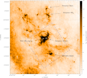
Figure 1: Visual extinction map towards the whole Aquila Rift / Serpens region derived by us from 2MASS data (see details in Schneider et al., 2010). The spatial resolution is 2^′ FWHM. The dashed blue rectangle indicates the Herschel coverage. It comprises the bright HII region W40 (white circle), the Serpens South cluster (white star), and the HII region Sh2-62, associated with the young star MWC297. The Aquila Rift corresponds to the large elongated structure from the northeast to the southwest. Emisson from the Galactic plane is seen in the southeast corner.

2 Observations

The observations were performed in the parallel mode of Herschel with a scanning speed of 60^′′/sec, which allows photometric imaging with SPIRE at 250, 350, and 500 $\mu$m and PACS at 70 and 160 $\mu$m. Two cross-linked scan maps were performed for a final coverage of $\sim 3.3^{\circ}\times 3.3^{\circ}$ (see Fig. 1).

The SPIRE data were reduced using HIPE version 2.0 and modified pipeline scripts; see Griffin et al. (2010) for the in-orbit performance and scientific capabilities, and Swinyard et al. (2010) for calibration methods and accuracy. A median baseline was applied to the maps for each scan leg, and the naive mapper was used as a mapmaking algorithm. The PACS data were reduced in HIPE 3.0. We used an updated version of the calibration files following the most recent prescriptions of the PACS ICC (see Könyves et al., 2010 for details). Multiresolution median and second-order deglitching, as well as a high-pass filtering over the full scan leg length, were applied. The final PACS maps were created using the photProject task, which performs simple projection of the data cube on the map grid.

The resulting PACS maps are displayed in Fig. 2. Owing to the rapid mapping speed, the resulting point spread functions (PSFs) are elongated in the scan directions leading to cross-like shapes of the PSFs with expected sizes of 5.9^′′$\times$12.2^′′ at 70$\,\mu$m and 11.6^′′$\times$15.7^′′ at 160$\,\mu$m. The resulting rms in these maps ranges from 50 to 1000 mJy/beam at 70$\,\mu$m and from 120 to 2200 mJy/beam at 160$\,\mu$m, depending on the level of background in the map. It is in the W40/Sh2-64 HII region that the background level is the highest.

3 Overview and distance of the Aquila Rift complex

The Aquila Rift is a coherent, $5^{\circ}$ long feature above the Galactic plane at l=$28^{\circ}$, clearly visible on an extinction map derived from the reddening of stars in 2MASS (Fig. 1). A distance of 225$\,\pm\,$55 pc has been derived for this extinction wall, using spectro-photometric studies of the optically visible stars (Straižys et al., 2003). This distance is very similar to the usually adopted distance of 260$\,\pm\,$37 pc for the Serpens star-forming region, located only $3^{\circ}$ north (Straižys et al., 1996).

On the other hand, the most active and main extinction feature in the 2MASS extinction map is associated with the HII region W40/Sh2-64, which has so far been considered to be at a distance ranging from 100 and 700 pc depending on author (Smith et al., 1985; Vallee, 1987 and references therein). These distance estimates are mostly based on kinematical distances that have large uncertainties. W40 could therefore be at the same distance as Serpens. Recently, Gutermuth et al. (2008) reported Spitzer observations of an embedded cluster, referred to as Serpens South, in the Aquila Rift region. This cluster is located very close in projection on the sky to W40 (see Fig. 1) and thus seems to be part of the W40 region. Gutermuth et al. (2008) proposed that the Serpens South cluster should be part of Serpens since it has the same velocity ($6$ km/s). The molecular cloud associated with W40 and traced by CII recombination lines and CO (Zeilik & Lada, 1978) has a velocity ranging from 4.5 to 6.5 km/s, which is also roughly the same as Serpens. More recent N₂H⁺ observations of the entire W40/Serpens South region confirm similar velocities in the whole region with velocity differences of only $\sim\,2\,$km/s (Maury et al. in prep). It is therefore more straightforward to consider that the W40 region is a single complex at the same distance as Serpens. This distance also suits the MWC297 / Sh2-62 region since the young 10 $M_{\odot}$ star MWC297 itself has an accepted distance of 250 pc (Drew et al., 1997). It is finally worth noting that the visual extinction map by Cambrésy (1999) derived from optical star counts and only tracing the first layer of the extinction wall has exactly the same global aspect as the 2MASS extinction map of Fig. 1, suggesting that both Serpens Main and the W40 / Aquila Rift / MWC297 region are associated with this extinction wall at 260 pc. We thus adopt the distance of 260 pc for the entire region in the following.

The 2MASS extinction map and the Herschel images (see Appendix for PACS images and Könyves et al., 2010 for SPIRE images) clearly show a massive cloud associated with W40. This cloud corresponds to G28.74+3.52 in (Zeilik & Lada, 1978) and has a mass of $1.1\times 10^{4}\,$$M_{\odot}$(derived from our 2MASS extinction map). The cloud associated with MWC297 is less massive ($4.1\times 10^{3}\,$$M_{\odot}$), and we obtain a total mass of 3.1$\times 10^{4}\,$$M_{\odot}$ for the whole area covered by Herschel.

2

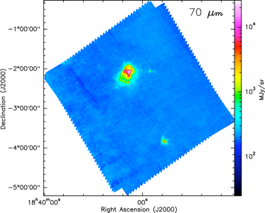
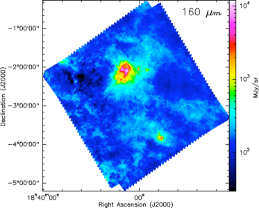
Figure 2: PACS 70$\,\mu$m (left) and 160$\,\mu$m (right) images of the Aquila field. See details about data reduction and map making in Sect. 2 and in Könyves et al. (2010). The corresponding SPIRE 250, 350, and 500$\,\mu$m images are shown in Könyves et al. (2010).

3

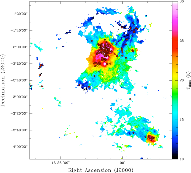
Figure 3: Distribution map of the 201 Herschel YSOs selected in Sect. 4.1, over-plotted on the map of dust temperature. The dust temperature map was derived from graybody fits to the Herschel data (see details in Könyves et al., 2010).

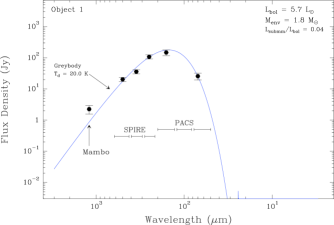
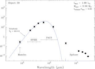
Figure 4: Spectral energy distributions of a newly discovered bright Class 0 (left panel) and of a weaker Class 0 object (right panel), which was previously detected with Spitzer in Gutermuth et al. (2008).

4 Results and analysis

4.1 Source detection and identification of protostars

A systematic source detection was performed on all 5 Herschel bands using getsources (Men’shchikov et al., 2010). This code uses a method based on a multiscale decomposition of the images to disentangle the emission of a population of spatially coherent sources in an optimized way in all bands simultaneously. We built a sample of the best candidate protostars for the whole field. These sources are clearly detected in all Herschel bands (high significance level), and we require a detection at the shortest Herschel wavelength, 70$\,\mu$m (or 24$\,\mu$m when Spitzer data were available), to distinguish YSOs from starless cores. Since the 24 and 70$\,\mu$m emission should only trace warm dust from the inner regions of the YSO envelopes, these sources can be safely interpreted as protostars. The 70$\,\mu$m fluxes have even been recently recognized as a very good tracer of protostellar luminosities (Dunham et al., 2008). On the other hand, in the PDR region of W40 some extended emission from warm dust at the HII region interface could contaminate this YSO detection criterium. To avoid too stringent a contamination from this extended emission, we selected only sources with an FWHM size smaller than 40^′′ at 70$\,\mu$m. Also, we had to make a source detection using a large pixel size of 6^′′, which is good enough for starless cores mostly detected in the SPIRE bands but not perfect to sample the spatial resolution at 70$\,\mu$m and properly disentangle possible multiple protostellar sources. A more precise detection could only be achieved in a reduced area in the Serpens South region (see Sect. 4.4).

A large number of compact sources are clearly seen in the 70$\,\mu$m map down to the sensitivity limit of the survey. In the whole Aquila field, 201 YSOs were detected with getsources. The best achieved rms (50 mJy/beam) in the Aquila 70$\,\mu$m map in the lowest background regions corresponds to a 5$\,\sigma$ detection level in terms of protostar luminosity of 0.05 $L_{\odot}$ using the Dunham et al. (2008) relationship. In contrast, in the highest background regions, the 5$\,\sigma$ detection level is then as high as 1.0 $L_{\odot}$. To account for the variable background level in Aquila, we performed simulations to evaluate the final completeness level of the YSO detection and obtained a 90 % completeness level of $\sim$0.2 $L_{\odot}$ (see Könyves et al., 2010), which is compatible with the above rough estimates using Dunham et al. (2008).

4.2 Spatial distribution of the protostars

We plotted in Fig. 3 the spatial distribution of the Herschel sample of 201 YSOs overlaid on the map of the dust temperature derived from a simple graybody fit of the Herschel data (see details in Könyves et al., 2010). It is clear that the W40 region corresponds to the most active star-forming region in the Herschel coverage with 90 % of the detected protostars. A second, much less rich, site corresponds to MWC297 with 8 % of the protostars, and another site to the east of W40 can be tentatively identified with very few candidate protostars.

4.3 Basic properties of the protostars: $M_{\rm env}$ and $L_{\rm bol}$

For each source an SED was built using the 5 bands of Herschel, as well as Spitzer photometry (Gutermuth et al., 2008) and MAMBO 1.2mm data (Maury et al. in prep) when available. These SEDs were systematically fitted using graybody functions to derive $M_{\rm env}$ in a systematic way, while the basic properties $L_{\rm bol}$, $L^{\rm\lambda>350}_{\rm submm}$, and $T_{\rm bol}$ were obtained by simple integrations of the SEDs. Two representative SEDs are displayed in Fig. 4 with a newly discovered Class 0 object and a weaker Class 0 source, which has a Spitzer counterpart in Gutermuth et al. (2008).

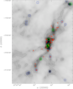
Figure 5: Herschel SPIRE 350$\mu$m image of the Serpens South region with the distribution of Herschel candidate protostars (blue circles) from the whole field extraction, of the 7 newly discovered Class 0 protostars (green circles), and of the Spitzer YSOs (red crosses; Gutermuth et al., 2008).

4.4 A close-up view of the Serpens South region

To go one step further in the identification and characterization of the Herschel protostars, we performed a more detailed analysis of the sources in a small area around the Serpens South cluster. In this area, we made a dedicated getsources source extraction using a smaller size pixel of 3^′′, and we could compare these first results with the Spitzer protostar population by Gutermuth et al. (2008). We used getsources on 8 bands from 8 to 1200$\,\mu$m by adding the 8 and 24$\,\mu$m Spitzer and the 1.2mm MAMBO data to the 5 Herschel bands.

A synthesized view of these first results based on this novel panchromatic analysis of infrared to millimeter range data for this area is given in Fig. 5. It shows the distribution of Herschel protostars compared to the Spitzer sources. The first analysis of this field indicates that even in a highly clustered region like Serpens South, a significant population of protostars were found to be missing by pure near and mid-infrared imaging with as many as 7 newly detected Class 0 objects in this field. We also note that the Spitzer protostars (most of these not detected with Herschel) probably correspond to evolved or low-luminosity Class I objects.

5 Global view of the protostellar population in Aquila

Using the basic properties derived in Sect. 4.3, we can draw the first picture of the property space Herschel is going to cover thanks to its unprecedentedly sensitive and high spatial resolution in the far-infrared.

In Fig. 6 we plotted the location of the 201 Herschel YSOs obtained in the entire field in a $M_{\rm env}-L_{\rm bol}$ evolutionary diagram used to compare observed properties with theoretical evolutionary models or tracks. The displayed tracks represent the expected evolution of protostars of masses 0.2, 0.6, 2.0, and 8.0 $M_{\odot}$ from the earliest times of accretion (upper left part of the diagram) to the time of 50 % mass accreted (conceptual limit between Class 0 and Class I YSOs), and the time for 90 % mass accreted (see Bontemps et al., 1996; Saraceno et al., 1996; André et al., 2000, 2008). In this plot, we distinguished objects with an $L^{\rm\lambda>350}_{\rm submm}/L^{\rm 70-500}_{\rm bol}$ higher than 0.03 which could be safely recognized as Class 0 objects, from YSOs with $L^{\rm\lambda>350}_{\rm submm}/L^{\rm 70-500}_{\rm bol}$ lower than 0.01 which are proposed to be Class I sources. The intermediate objects with $0.03>L^{\rm\lambda>350}_{\rm submm}/L^{\rm 70-500}_{\rm bol}>0.01$ should be seen as objects with an uncertain classification. A forthcoming analysis will resolve their nature by building complete SEDs including Spitzer data for a large part of the Aquila field. So far we could safely classify objects only in the reduced area of Serpens South (Sect. 4.4). In this subfield, we verified that objects with $L^{\rm\lambda>350}_{\rm submm}/L^{\rm 70-500}_{\rm bol}>0.03$ and $T^{\rm 70-500}_{\rm bol}<27\,$K using the reduced (only the 5 Herschel bands from 70 to 500$\,\mu$m) SED coverage are indeed all found to be Class 0 objects based on the full coverage from 8$\,\mu$m to 1.2 mm. We see that the obtained location of Class 0 and Class I YSOs is compatible with the 50 % mass accreted limit. Imposing Class 0 objects to have to be above this limit (dashed line in Fig. 6), we finally found between 45 (for $T^{\rm 70-500}_{\rm bol}<27\,$K) and 60 ($L^{\rm\lambda>350}_{\rm submm}/L^{\rm 70-500}_{\rm bol}>0.03$) Class 0 objects in the entire field of Aquila.

In conclusion, even if the precise locations of the Herschel protostars in this diagram are seen as a preliminary result and will be updated with a more complete analysis and source detection, our early results clearly indicate that Herschel is a powerful tool for probing the virtually unexplored area of the physical properties of the earliest stages of protostellar evolution.

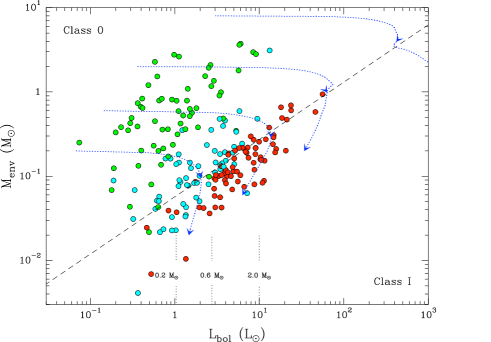
Figure 6: Distribution of the Herschel sample of protostars in the protostellar evolutionary diagram $M_{\rm env}-L_{\rm bol}$. The green and red circles are for the Class 0 and Class I protostars with $L^{\rm\lambda>350}_{\rm submm}/L^{\rm 70-500}_{\rm bol}>0.03$ and $<0.01$ (see text), respectively. The intermediate, more uncertain cases with $0.03>L^{\rm\lambda>350}_{\rm submm}/L^{\rm 70-500}_{\rm bol}>0.01$ are displayed as light blue circles. The evolutionary tracks for 0.2, 0.6, 2.0, and 8.0 $M_{\odot}$ are displayed as dotted curves. The formal separation between Classes 0 and I in this diagram corresponds to 50 % of the mass accreted, which corresponds to the locii of the first arrows on the curves (see also the dashed separating line). The second arrows on the curves indicate 90 % of the mass accreted.