A Distributed Newton Method for Network Utility Maximization

Most existing work uses dual decomposition and first-order methods to solve Network Utility Maximization (NUM) problems in a distributed manner, which suffer from slow rate of convergence properties. This paper develops an alternative distributed Newton-type fast converging algorithm for solving NUM problems with self-concordant utility functions. By using novel matrix splitting techniques, both primal and dual updates for the Newton step can be computed using iterative schemes in a decentralized manner. We propose a stepsize rule and provide a distributed procedure to compute it in finitely many iterations. The key feature of our direction and stepsize computation schemes is that both are implemented using the same distributed information exchange mechanism employed by first order methods. We show that even when the Newton direction and the stepsize in our method are computed within some error (due to finite truncation of the iterative schemes), the resulting objective function value still converges superlinearly in terms of primal iterations to an explicitly characterized error neighborhood. Simulation results demonstrate significant convergence rate improvement of our algorithm relative to the existing first-order methods based on dual decomposition.

1 Introduction

Most of today’s communication networks are large-scale and comprise of agents with heterogeneous preferences. Lack of access to centralized information in such networks necessitate design of distributed control algorithms that can operate based on locally available information. Some applications include routing and congestion control in the Internet, data collection and processing in sensor networks, and cross-layer design in wireless networks. This work focuses on the rate control problem in wireline networks, which can be formulated in the Network Utility Maximization (NUM) framework proposed in [22] (see also [25], [33], and [11]). NUM problems are characterized by a fixed network and a set of sources, which send information over the network along predetermined routes. Each source has a local utility function over the rate at which it sends information. The goal is to determine the source rates that maximize the sum of utilities subject to link capacity constraints. The standard approach for solving NUM problems relies on using dual decomposition and subgradient (or first-order) methods, which through a price exchange mechanism among the sources and the links yields algorithms that can operate on the basis of local information. One major shortcoming of this approach is the slow rate of convergence.

In this paper, we propose a novel Newton-type second-order method for solving the NUM problem in a distributed manner, which leads to significantly faster convergence. Our approach involves transforming the inequality constrained NUM problem to an equality-constrained one through introducing slack variables and logarithmic barrier functions, and using an equality-constrained Newton method for the reformulated problem. There are two challenges in implementing this method in a distributed manner. First challenge is the computation of the Newton direction. This computation involves a matrix inversion, which is costly and requires global information. We solve this problem by using an iterative scheme based on a novel matrix splitting technique. Since the objective function of the (equality-constrained) NUM problem is separable, i.e., it is the sum of functions over each of the variables, this splitting enables computation of the Newton direction using decentralized algorithms based on limited “scalar” information exchange between sources and links. This exchange involves destinations iteratively sending route prices (aggregated link prices or dual variables along a route) to the sources, and sources sending the route price scaled by the Hessian to the links along its route. Therefore, our algorithm has comparable level of information exchange with the first-order methods applied to the NUM problem.

The second challenge is related to the computation of a stepsize rule that can guarantee local superlinear convergence of the primal iterations. Instead of the iterative backtracking rules typically used with Newton methods, we propose a stepsize rule which is inversely proportional to the inexact Newton decrement (where the inexactness arises due to errors in the computation of the Newton direction) if this decrement is above a certain threshold and takes the form of a pure Newton step otherwise. Computation of the inexact Newton decrement involves aggregating local information from the sources and links in the network. We propose a novel distributed procedure for computing the inexact Newton decrement in finite number of steps using again the same information exchange mechanism employed by first order methods.

Since our method uses iterative schemes to compute the Newton direction, exact computation is not feasible. Another major contribution of our work is to consider a truncated version of this scheme, allow error in stepsize computation and present convergence rate analysis of the constrained Newton method when the stepsize and the Newton direction are estimated with some error. We show that when these errors are sufficiently small, the value of the objective function converges superlinearly in terms of primal iterations to a neighborhood of the optimal objective function value, whose size is explicitly quantified as a function of the errors and bounds on them.

Our work contributes to the growing literature on distributed optimization and control of multi-agent networked systems. There are two standard approaches for designing distributed algorithms for such problems. The first approach, as mentioned above, uses dual decomposition and subgradient methods, which for some problems including NUM problems lead to iterative distributed algorithms (see [22], [25]). Subsequent work by Athuraliya and Low in [1] use diagonal scaling to approximate Newton steps to speed up the subgradient algorithm while maintaining their distributed nature. Despite improvements in speed over the first-order methods, as we shall see, the performance of this modified algorithm does not achieve the rate gains obtained by second-order methods.

The second approach involves considering consensus-based schemes, in which agents exchange local estimates with their neighbors with the goal of aggregating information over an exogenous (fixed or time-varying) network topology (see [34], [8], [29], [35], [17], [31], [18] and [32]). It has been shown that under some mild assumption on the connectivity of the graph and updating rules, the distance from the vector formed by current estimates to consensus diminishes linearly. Consensus schemes can be used to compute the average of local values or more generally as a building block for developing distributed optimization algorithms with linear/sublinear rate of convergence ([28]). The stepsize for the distributed Newton method can be computed using consensus type of algorithms. However, the distributed Newton method achieves quadratic rate of convergence for the primal iterations, using consensus results in prohibitively slow stepsize computation at each iteration, and is hence avoided in our method.

Other than the papers cited above, our paper is also related to [4], [23], [6] and [18]. In [4], Bertsekas and Gafni studied a projected Newton method for optimization problems with twice differentiable objective functions and simplex constraints. They proposed finding the Newton direction (exactly or approximately) using a conjugate gradient method. This work showed that when applied to multi-commodity network flow problems, the conjugate gradient iterations can be obtained using simple graph operations, however did not investigate distributed implementations. Similarly, in [23], Klincewicz proposed a Newton method for network flow problems that computes the dual variables at each step using an iterative conjugate gradient algorithm. He showed that conjugate gradient iterations can be implemented using a “distributed” scheme that involves simple operations and information exchange along a spanning tree. Spanning tree based computations involve passing all information to a centralized node and may therefore be restrictive for NUM problems which are characterized by decentralized (potentially autonomous) sources.

In [6], the authors have developed a distributed Newton-type method for the NUM problem using a belief propagation algorithm. Belief propagation algorithms, while performing well in practice, lack systematic convergence guarantees. Another recent paper [18] studied a Newton method for equality-constrained network optimization problems and presented a convergence analysis under Lipschitz assumptions. In this paper, we focus on an inequality-constrained problem, which is reformulated as an equality-constrained problem using barrier functions. Therefore, this problem does not satisfy Lipschitz assumptions. Instead, we assume that the utility functions are self-concordant and present a novel convergence analysis using properties of self-concordant functions.

Our analysis for the convergence of the algorithm also relates to work on convergence rate analysis of inexact Newton methods (see [14], [20]). These works focus on providing conditions on the amount of error at each iteration relative to the norm of the gradient of the current iterate that ensures superlinear convergence to the exact optimal solution (essentially requiring the error to vanish in the limit). Even though these analyses can provide superlinear rate of convergence, the vanishing error requirement can be too restrictive for practical implementations. Another novel feature of our analysis is the consideration of convergence to an approximate neighborhood of the optimal solution. In particular, we allow a fixed error level to be maintained at each step of the Newton direction computation and show that superlinear convergence is achieved by the primal iterates to an error neighborhood, whose size can be controlled by tuning the parameters of the algorithm. Hence, our work also contributes to the literature on error analysis for inexact Newton methods.

The rest of the paper is organized as follows: Section 2 defines the problem formulation and related transformations. Section 3 describes the exact constrained primal-dual Newton method for this problem. Section 4 presents a distributed iterative scheme for computing the dual Newton step and the distributed inexact Newton-type algorithm. Section 5 contains the rate of convergence analysis for our algorithm. Section 6 presents simulation results to demonstrate convergence speed improvement of our algorithm to the existing methods with linear convergence rates. Section 7 contains our concluding remarks.

Basic Notation and Notions:

A vector is viewed as a column vector, unless clearly stated otherwise. We write $\mathbb{R}_{+}$ to denote the set of nonnegative real numbers, i.e., $\mathbb{R}_{+}=[0,\infty)$. We use subscripts to denote the components of a vector and superscripts to index a sequence, i.e., $x_{i}$ is the $i^{th}$ component of vector $x$ and $x^{k}$ is the $k$th element of a sequence. When $x_{i}\geq 0$ for all components $i$ of a vector $x$, we write $x\geq 0$.

For a matrix $A$, we write $A_{ij}$ to denote the matrix entry in the $i^{th}$ row and $j^{th}$ column, and $[A]_{i}$ to denote the $i^{th}$ column of the matrix $A$, and $[A]^{j}$ to denote the $j^{th}$ row of the matrix $A$. We write $I(n)$ to denote the identity matrix of dimension $n\times n$. We use $x^{\prime}$ and $A^{\prime}$ to denote the transpose of a vector $x$ and a matrix $A$ respectively. For a real-valued function $f:X\rightarrow\mathbb{R}$, where $X$ is a subset of $\mathbb{R}^{n}$, the gradient vector and the Hessian matrix of $f$ at $x$ in $X$ are denoted by $\nabla f(x)$ and $\nabla^{2}f({x})$ respectively. We use the vector $e$ to denote the vector of all ones.

A real-valued convex function $g:X\rightarrow\mathbb{R}$, where $X$ is a subset of $\mathbb{R}$, is self-concordant if it is three times continuously differentiable and $|{g}^{\prime\prime\prime}(x)|\leq 2{g}^{\prime\prime}(x)^{\frac{3}{2}}$ for all $x$ in its domain. For real-valued functions in $\mathbb{R}^{n}$, a convex function $g:X\rightarrow\mathbb{R}$, where $X$ is a subset of $\mathbb{R}^{n}$, is self-concordant if it is self-concordant along every direction in its domain, i.e., if the function $\tilde{g}(t)=g(x+tv)$ is self-concordant in $t$ for all $x$ and $v$. Operations that preserve self-concordance property include summing, scaling by a factor $\alpha\geq 1$, and composition with affine transformation (see [9] Chapter $9$ for more details).

2 Network Utility Maximization Problem

We consider a network represented by a set $\mathcal{L}=\{1,...,L\}$ of (directed) links of finite nonzero capacity given by $c=[c_{l}]_{l\in\mathcal{L}}$ with $c>0$. The network is shared by a set $\mathcal{S}=\{1,...,S\}$ of sources, each of which transmits information along a predetermined route. For each link $l$, let $S(l)$ denote the set of sources use it. For each source $i$, let $L(i)$ denote the set of links it uses. We also denote the nonnegative source rate vector by $s=[s_{i}]_{i\in\mathcal{S}}$. The capacity constraint at the links can be compactly expressed as

$$Rs\leq c,$$

where $R$ is the routing matrix of dimension $L\times S$, i.e.,

$$R_{ij}=\left\{\begin{array}[]{rl}1&\mbox{if link $i$ is on the route of source $j$},\\ 0&\mbox{otherwise}.\end{array}\right.$$ (1)

We associate a utility function $U_{i}:\mathbb{R}_{+}\to\mathbb{R}$ with each source $i$, i.e., $U_{i}(s_{i})$ denotes the utility of source $i$ as a function of the source rate $s_{i}$. We assume the utility functions are additive, such that the overall utility of the network is given by $\sum_{i=1}^{S}U_{i}(s_{i})$. Thus the Network Utility Maximization(NUM) problem can be formulated as

maximize $$\sum_{i=1}^{S}U_{i}(s_{i})$$ (2)

subject to $$Rs\leq c,$$

$$s\geq 0.$$

We adopt the following assumption.

Assumption 1.

The utility functions $U_{i}:\mathbb{R}_{+}\to\mathbb{R}$ are strictly concave, monotonically nondecreasing on $(0,\infty)$. The functions $-U_{i}:\mathbb{R}_{+}\to\mathbb{R}$ are self-concordant on $(0,\infty)$.

The self-concordance assumption is satisfied by standard utility functions considered in the literature, for instance logarithmic, i.e., weighted proportional fair utility functions [33], and concave quadratic utility functions, and is adopted here to allow a self-concordant analysis in establishing local quadratic convergence. We use $h(x)$ to denote the (negative of the) objective function of problem (2), i.e., $h(x)=-\sum_{i=1}^{S}U_{i}({x_{i}})$, and $h^{*}$ to denote the (negative of the) optimal value of this problem. Since $h(x)$ is continuous and the feasible set of problem (2) is compact, it follows that problem (2) has an optimal solution, and therefore $h^{*}$ is finite. Moreover, the interior of the feasible set is nonempty, i.e., there exists a feasible solution $x$ with $x_{i}=\frac{\underline{c}}{S+1}$ for all $i\in\mathcal{S}$ with $\underline{c}>0$.

To facilitate the development of a distributed Newton-type method, we consider a related equality-constrained problem by introducing nonnegative slack variables $[y_{l}]_{l\in\mathcal{L}}$ for the capacity constraints, defined by

$$\sum_{j=1}^{S}R_{lj}s_{j}+{y}_{l}=c_{l}\quad\textrm{for }l=1,2\ldots L,$$ (3)

and logarithmic barrier functions for the nonnegativity constraints (which can be done since the feasible set of (2) has a nonempty interior). We denote the new decision vector by $x=([s_{i}]^{\prime}_{i\in\mathcal{S}},[y_{l}]^{\prime}_{l\in\mathcal{L}})^{\prime}$. This problem can be written as

minimize $$-\sum_{i=1}^{S}U_{i}({x_{i}})-\mu\sum_{i=1}^{S+L}\log{({x_{i}})}$$ (4)

subject to $$A{x}=c,$$

where $A$ is the $L\times(S+L)$-dimensional matrix given by

$$A=[R\quad I(L)],$$ (5)

and $\mu$ is a nonnegative barrier function coefficient. We use $f(x)$ to denote the objective function of problem (4), i.e.,

$$f(x)=-\sum_{i=1}^{S}U_{i}({x_{i}})-\mu\sum_{i=1}^{S+L}\log{({x}_{i})},$$ (6)

and $f^{*}$ to denote the optimal value of this problem, which is finite for positive $\mu$.

By Assumption 1, the function $f(x)$ is separable, strictly convex, and has a positive definite diagonal Hessian matrix on the positive orthant. The function $f(x)$ is also self-concordant for $\mu\geq 1$, since both summing and scaling by a factor $\mu\geq 1$ preserve self-concordance property.

We write the optimal solution of problem (4) for a fixed barrier function coefficient $\mu$ as $x(\mu)$. One can show that as the barrier function coefficient $\mu$ approaches 0, the optimal solution of problem (4) approaches that of problem (2), when the constraint set in (2) has nonempty interior and is convex [3], [15]. Hence by continuity from Assumption 1, $h(x(\mu))$ approaches $h^{*}$. Therefore, in the rest of this paper, unless clearly stated otherwise, we study iterative distributed methods for solving problem (4) for a given $\mu$. In order to preserve the self-concordance property of the function $f$, which will be used in our convergence analysis, we first develop a Newton-type algorithm for $\mu\geq 1$. In Section 5.3, we show that problem (4) for any $\mu>0$ can be tackled by solving two instances of problem (4) with different coefficients $\mu\geq 1$, leading to a solution $x(\mu)$ that satisfies $\frac{h(x(\mu))-h^{*}}{h^{*}}\leq a$ for any positive scalar $a$.

3 Exact Newton Method

For each fixed $\mu$, problem (4) is feasible and has a convex objective function, affine constraints, and a finite optimal value $f^{*}$. Therefore, we can use a strong duality theorem to show that, for problem (4), there is no duality gap and there exists a dual optimal solution (see [5]). Moreover, since matrix $A$ has full row rank,

we can use a (feasible start) equality-constrained Newton method to solve problem (4)(see [9] Chapter 10).

3.1 Feasible Initialization

We initialize the algorithm with some feasible and strictly positive vector $x^{0}$. For example, one such initial vector is given by

$$x_{i}^{0} =\frac{\underline{c}}{S+1}\quad\textrm{for }i=1,2\ldots S,$$ (7)

$$\quad x_{l+S}^{0} =c_{l}-\sum_{j=1}^{S}R_{lj}\frac{\underline{c}}{S+1}\quad\textrm{for }l=1,2\ldots L,$$

where $c_{l}$ is the finite capacity for link $l$, $\underline{c}$ is the minimum (nonzero) link capacity, $S$ is the total number of sources in the network, and $R$ is routing matrix [cf. Eq. (1)].

3.2 Iterative Update Rule

Given an initial feasible vector $x^{0}$, the algorithm generates the iterates by

$$x^{k+1}=x^{k}+d^{k}\Delta x^{k},$$ (8)

where $d^{k}$ is a positive stepsize, $\Delta x^{k}$ is the (primal) Newton direction given as the solution of the following system of linear equations:.

$$\left(\begin{array}[]{cc}\nabla^{2}f({x}^{k})&A^{\prime}\\ A&0\end{array}\right)\left(\begin{array}[]{c}\Delta x^{k}\\ w^{k}\end{array}\right)=-\left(\begin{array}[]{c}\nabla f({x}^{k})\\ 0\end{array}\right).$$ (15)

We will refer to $x^{k}$ as the primal vector and $w^{k}$ as the dual vector (and their components as primal and dual variables respectively). We also refer to $w^{k}$ as the price vector since the dual variables $[w_{l}^{k}]_{l\in\mathcal{L}}$ associated with the link capacity constraints can be viewed as prices for using links. For notational convenience, we will use $H_{k}=\nabla^{2}f({x}^{k})$ to denote the Hessian matrix in the rest of the paper.

Solving for $\Delta x^{k}$ and $w^{k}$ in the preceding system yields

$$\Delta x^{k}=-H_{k}^{-1}(\nabla f(x^{k})+A^{\prime}w^{k}),$$ (16)

$$(AH_{k}^{-1}A^{\prime})w^{k}=-AH_{k}^{-1}\nabla f(x^{k}).$$ (17)

This system has a unique solution for all $k$. To see this, note that the matrix $H_{k}$ is a diagonal matrix with entries

$$(H_{k})_{ii}=\left\{\begin{array}[]{ccc}-\frac{\partial^{2}U_{i}(x_{i}^{k})}{\partial x_{i}^{2}}+\frac{\mu}{(x_{i}^{k})^{2}}&1\leq i\leq S,\\ \frac{\mu}{(x_{i}^{k})^{2}}&S+1\leq i\leq S+L.\end{array}\right.$$ (20)

By Assumption 1, the functions $U_{i}$ are strictly concave, which implies $\frac{\partial^{2}U_{i}(x_{i}^{k})}{\partial x_{i}^{2}}\leq 0$. Moreover, the primal vector $x^{k}$ is bounded (since the method maintains feasibility) and, as we shall see in Section 4.4, can be guaranteed to remain strictly positive by proper choice of stepsize. Therefore, the entries $(H_{k})_{ii}>0$ and are well-defined for all $i$, implying that the Hessian matrix $H_{k}$ is invertible. Due to the structure of $A$ [cf. Eq. (5)], the column span of $A$ is the entire space $\mathbb{R}^{L}$, and hence the matrix $AH_{k}^{-1}A^{\prime}$ is also invertible. This shows that the preceding system of linear equations can be solved uniquely for all $k$.

The objective function $f$ is separable in $x_{i}$, therefore given the vector $w^{k}_{l}$ for $l$ in $L(i)$, the Newton direction $\Delta x^{k}_{i}$ can be computed by each source $i$ using local information available to that source. However, the computation of the vector $w^{k}$ at a given primal solution $x^{k}$ cannot be implemented in a decentralized manner since the evaluation of the matrix inverse $(AH_{k}^{-1}A^{\prime})^{-1}$ requires global information. The following section provides a distributed inexact Newton method, based on computing the vector $w^{k}$ using a decentralized iterative scheme.

4 Distributed Inexact Newton Method

In this section, we introduce a distributed Newton method using ideas from matrix splitting in order to compute the dual vector $w^{k}$ at each $k$ using an iterative scheme. Before proceeding to present the details of the algorithm, we first introduce some preliminaries on matrix splitting.

4.1 Preliminaries on Matrix Splitting

Matrix splitting can be used to solve a system of linear equations given by

$$Gy=a,$$

where $G$ is an $n\times n$ matrix and $a$ is an $n$-dimensional vector. Suppose that the matrix $G$ can be expressed as the sum of an invertible matrix $M$ and a matrix $N$, i.e.,

$$G=M+N.$$ (21)

Let $y_{0}$ be an arbitrary $n$-dimensional vector. A sequence $\{y^{k}\}$ can be generated by the following iteration:

$$y^{k+1}=-M^{-1}Ny^{k}+M^{-1}a.$$ (22)

It can be seen that the sequence $\{y^{k}\}$ converges as $k\to\infty$ if and only if the spectral radius of the matrix $M^{-1}N$ is strictly bounded above by 1. When the sequence $\{y^{k}\}$ converges, its limit $y^{*}$ solves the original linear system, i.e., $Gy^{*}=a$ (see [2] and [13] for more details). Hence, the key to solving the linear equation via matrix splitting is the bound on the spectral radius of the matrix $M^{-1}N$. Such a bound can be obtained using the following result (see Theorem 2.5.3 from [13]).

Theorem 4.1.

Let $G$ be a real symmetric matrix. Let $M$ and $N$ be matrices such that $G=M+N$ and assume that $M$ is invertible and both matrices $M+N$ and $M-N$ are positive definite. Then the spectral radius of $M^{-1}N$, denoted by $\rho(M^{-1}N)$, satisfies $\rho(M^{-1}N)<1$.

By the above theorem, if $G$ is a real, symmetric, positive definite matrix and $M$ is a nonsingular matrix, then one sufficient condition for the iteration (22) to converge is that the matrix $M-N$ is positive definite. This can be guaranteed using Gershgorin Circle Theorem, which we introduce next (see [37] for more details).

Theorem 4.2.

(Gershgorin Circle Theorem) Let $G$ be an $n\times n$ matrix, and define $r_{i}(G)=\sum_{j\neq i}|G_{ij}|$. Then, each eigenvalue of $G$ lies in one of the Gershgorin sets $\{\Gamma_{i}\}$, with $\Gamma_{i}$ defined as disks in the complex plane, i.e.,

$$\Gamma_{i}=\{z\in\mathbb{C}\mid|z-G_{ii}|\leq r_{i}(G)\}.$$

One corollary of the above theorem is that if a matrix G is strictly diagonally dominant, i.e., $|G_{ii}|>\sum_{j\neq i}|G_{ij}|$, and $G_{ii}>0$ for all $i$, then the real parts of all the eigenvalues lie in the positive half of the real line, and thus the matrix is positive definite. Hence a sufficient condition for the matrix $M-N$ to be positive definite is that $M-N$ is strictly diagonally dominant with strictly positive diagonal entries.

4.2 Distributed Computation of the Dual Vector

We use the matrix splitting scheme introduced in the preceding section to compute the dual vector $w^{k}$ in Eq. (17) in a distributed manner. Let $D_{k}$ be a diagonal matrix, with diagonal entries

$$(D_{k})_{ll}=(AH_{k}^{-1}A^{\prime})_{ll},$$ (23)

and matrix $B_{k}$ be given by

$$B_{k}=AH_{k}^{-1}A^{\prime}-D_{k}.$$ (24)

Let matrix $\bar{B}_{k}$ be a diagonal matrix, with diagonal entries

$$(\bar{B}_{k})_{ii}=\sum_{j=1}^{L}(B_{k})_{ij}.$$ (25)

By splitting the matrix $AH_{k}^{-1}A^{\prime}$ as the sum of $D_{k}+\bar{B}_{k}$ and $B_{k}-\bar{B}_{k}$, we obtain the following result.

Theorem 4.3.

For a given $k>0$, let $D_{k}$, $B_{k}$, $\bar{B}_{k}$ be the matrices defined in Eqs. (23), (24) and (25). Let $w(0)$ be an arbitrary initial vector and consider the sequence $\{w(t)\}$ generated by the iteration

$$w(t+1)=(D_{k}+\bar{B}_{k})^{-1}(\bar{B}_{k}-B_{k})w(t)+(D_{k}+\bar{B}_{k})^{-1}(-AH_{k}^{-1}\nabla f(x^{k})),$$ (26)

for all $t\geq 0$. Then the spectral radius of the matrix $(D_{k}+\bar{B}_{k})^{-1}(B_{k}-\bar{B}_{k})$ is strictly bounded above by $1$ and the sequence $\{w(t)\}$ converges as $t\to\infty$, and its limit is the solution to Eq. (17).

Proof.

We split the matrix $AH_{k}^{-1}A^{\prime}$ as

$$(AH_{k}^{-1}A^{\prime})=(D_{k}+\bar{B}_{k})+(B_{k}-\bar{B}_{k})$$ (27)

and use the iterative scheme presented in Eqs. (21) and (22) to solve Eq. (17). For all $k$, both the real matrix $H_{k}$ and its inverse, $H_{k}^{-1}$, are positive definite and diagonal. The matrix $A$ has full row rank and is element-wise nonnegative. Therefore the product $AH_{k}^{-1}A^{\prime}$ is real, symmetric, element-wise nonnegative and positive definite. We let

$$Q_{k}=(D_{k}+\bar{B}_{k})-(B_{k}-\bar{B}_{k})=D_{k}+2\bar{B}_{k}-B_{k}$$ (28)

denote the difference matrix. By definition of $\bar{B}_{k}$ [cf. Eq. (25)], the matrix $2\bar{B}_{k}-B_{k}$ is diagonally dominant, with nonnegative diagonal entries. Moreover, due to strict positivity of the second derivatives of the logarithmic barrier functions, we have $(D_{k})_{ii}>0$ for all $i$. Therefore the matrix $Q_{k}$ is strictly diagonally dominant. By Theorem 4.2, such matrices are positive definite. Therefore, by Theorem 4.1, the spectral radius of the matrix $(D_{k}+\bar{B}_{k})^{-1}(B_{k}-\bar{B}_{k})$ is strictly bounded above by $1$. Hence the splitting scheme (27) guarantees the sequence $\{w(t)\}$ generated by iteration (26) to converge to the solution of Eq. (17). ∎

This provides an iterative scheme to compute the dual vector $w^{k}$ at each primal iteration $k$ using an iterative scheme. We will refer to the iterative scheme defined in Eq. (26) as the dual iteration.

There are many ways to split the matrix $AH_{k}^{-1}A^{\prime}$. The particular one in Eq. (27) is chosen here due to three desirable features. First it guarantees that the difference matrix $Q_{k}$ [cf. Eq. (28)] is strictly diagonally dominant, and hence ensures convergence of the sequence $\{w(t)\}$. Second, with this splitting scheme, the matrix $D_{k}+\bar{B}_{k}$ is diagonal, which eliminates the need for global information when calculating its inverse. The third feature enables us to study convergence rate of iteration (26) in terms of a dual (routing) graph which we introduce next.

Definition 1.

Consider a network $\mathcal{G}=\{\mathcal{L},\mathcal{S}\}$, represented by a set $\mathcal{L}=\{1,...,L\}$ of (directed) links, and a set $\mathcal{S}=\{1,...,S\}$ of sources. The links form a strongly connected graph, and each source sends information along a predetermined route. The weighted dual (routing) graph $\tilde{\mathcal{G}}=\{\tilde{\mathcal{N}},\tilde{\mathcal{L}}\}$, where $\tilde{\mathcal{N}}$ is the set of nodes, and $\tilde{\mathcal{L}}$ is the set of (directed) links defined by:
A. $\tilde{\mathcal{N}}=\mathcal{L}$;
B. A link is present between node $L_{i}$ to $L_{j}$ in $\tilde{\mathcal{G}}$ if and only if there is some common flow between $L_{i}$ and $L_{j}$ in $\mathcal{G}$.
C. The weight $\tilde{W}_{ij}$ on the link from node $L_{i}$ to $L_{j}$ is given by

$$\tilde{W}_{ij}=(D_{k}+\bar{B}_{k})^{-1}_{ii}(B_{k})_{ij}=(D_{k}+\bar{B}_{k})^{-1}_{ii}(AH_{k}^{-1}A^{\prime})_{ij}=(D_{k}+\bar{B}_{k})^{-1}_{ii}\sum_{s\in S(i)\cap S(j)}H_{ss}^{-1},$$

where the matrices $D_{k}$, $B_{k}$, and $\bar{B}_{k}$ are defined in Eqs. (23), (24) and (25).

One example of a network and its dual graph are presented in Figures 1 and 2. Note that the unweighted indegree and outdegree of a node are the same in the dual graph, however the weights are different depending on the direction of the links. The splitting scheme in Eq. (27) involves the matrix $(D_{k}+\bar{B}_{k})^{-1}(\bar{B}_{k}-B_{k})$, which is the weighted Laplacian matrix of the dual graph. The weighted out-degree of node $i$ in the dual graph, i.e., the diagonal entry $(D_{k}+\bar{B}_{k})^{-1}_{ii}\bar{B}_{ii}$ of the Laplacian matrix, can be viewed as a measure of the congestion level of a link in the original network since the neighbors in the dual graph represent links that share flows in the original network. We show in Section 5.1 that the spectral properties of the Laplacian matrix of the dual graph dictate the convergence speed of dual iteration (26).

Figure 1: A sample network. Each source-destination pair is displayed with the same color. We use $x_{i}$ to denote the flow corresponding to the $i^{th}$ source-destination pair and $L_{i}$ to denote the $i^{th}$ link.

Figure 2: Dual graph for the network in Figure 1, each link in this graph corresponds to the flows shared between the links in the original network.

We next rewrite iteration (26), analyze the information exchange required to implement it and develop a distributed computation procedure to calculate the dual vector. For notational convenience, we define the price of the route for source $i$, $\pi_{i}(t)$, as the sum of the dual variables associated with links used by source $i$ at the $t^{th}$ dual iteration, i.e., $\pi_{i}(t)=\sum_{l\in L(i)}w_{l}(t)$. Similarly, we define the weighted price of the route for source $i$, $\Pi_{i}(t)$, as the price of the route for source $i$ weighted by the $i$th diagonal element of the inverse Hessian matrix, i.e., $\Pi_{i}(t)=(H_{k}^{-1})_{ii}\sum_{l\in L(i)}w_{l}(t)$.

Lemma 4.4.

For each primal iteration $k$, the dual iteration (26) can be written as

$$w_{l}(t+1)= \frac{1}{(H_{k})^{-1}_{(S+l)(S+l)}+\sum_{i\in S(l)}\Pi_{i}(0)}\Big{(}\Big{(}\sum_{i\in S(l)}\Pi_{i}(0)-\sum_{i\in S(l)}(H_{k})_{ii}^{-1}\Big{)}w_{l}(t)-\sum_{i\in S(l)}\Pi_{i}(t)$$ (29)

$$+\sum_{i\in S(l)}(H_{k})_{ii}^{-1}w_{l}(t)-\sum_{i\in S(l)}(H_{k}^{-1})_{ii}\nabla_{i}f(x^{k})-(H_{k}^{-1})_{(S+l)(S+l)}\nabla_{S+l}f(x^{k})\Big{)},$$

where $\Pi_{i}(0)$ is the weighted price of the route for source $i$ when $w(0)=[1,1\ldots,1]^{\prime}$.

Proof.

Recall the definition of matrix $A$, i.e., $A_{li}=1$ for $i=1,2\ldots S$ if source $i$ uses link $l$, i.e., $i\in S(l)$, and $A_{li}=0$ otherwise. Therefore, we can write the price of the route for source $i$ as, $\pi_{i}(t)=\sum_{l=1}^{L}A_{li}w(t)_{l}=[A^{\prime}]^{i}w(t)$. Similarly, since the Hessian matrix $H_{k}$ is diagonal, the weighted price can be written as

$${\Pi_{i}(t)=(H_{k})_{ii}^{-1}[A^{\prime}]^{i}w(t)=[H_{k}^{-1}A^{\prime}]^{i}w(t).}$$ (30)

On the other hand, since $A=[R$ $I(L)]$, where $R$ is the routing matrix, we have

$$(AH^{-1}_{k}A^{\prime}w(t))_{l} =\sum_{i=1}^{S}([A]_{i}[H_{k}^{-1}A^{\prime}]^{i}w(t))_{l}+(H_{k}^{-1})_{(S+l)(S+l)}w_{l}(t)$$

$$=\sum_{i=1}^{S}A_{li}([H_{k}^{-1}A^{\prime}]^{i}w(t))+(H_{k}^{-1})_{(S+l)(S+l)}w_{l}(t).$$

Using the definition of the matrix $A$ one more time, this implies

$$(AH^{-1}_{k}A^{\prime}w(t))_{l} =\sum_{i\in S(l)}[H_{k}^{-1}A^{\prime}]^{i}w(t)+(H_{k}^{-1})_{(S+l)(S+l)}w_{l}(t)$$ (31)

$$=\sum_{i\in S(l)}\Pi_{i}(t)+(H_{k}^{-1})_{(S+l)(S+l)}w_{l}(t),$$

where the last equality follows from Eq. (30).

Using Eq. (24), the above relation implies that $((B_{k}+D_{k})w(t))_{l}=\sum_{i\in S(l)}\Pi_{i}(t)+(H_{k}^{-1})_{(S+l)(S+l)}w_{l}(t)$. We next rewrite $(\bar{B}_{k})_{ll}$. Using the fact that $w(0)=[1,1\ldots,1]^{\prime}$, we have

$$(AH^{-1}_{k}A^{\prime}w(0))_{l}=((B_{k}+D_{k})w(0))_{l}=\sum_{j=1}^{L}(B_{k})_{lj}+(D_{k})_{ll}.$$

Using the definition of $\bar{B}_{k}$ [cf. Eq. (25)], this implies

$$(\bar{B}_{k})_{ll} =\sum_{j=1}^{L}(B_{k})_{lj}=(AH^{-1}_{k}A^{\prime}w(0))_{l}-(D_{k})_{ll}$$

$$=\sum_{i\in S(l)}\Pi_{i}(0)+(H_{k}^{-1})_{(S+l)(S+l)}-(D_{k})_{ll}.$$

This calculation can further be simplified using

$$(D_{k})_{ll}=(AH_{k}^{-1}A^{\prime})_{ll}=\sum_{i\in S(l)}(H_{k})_{ii}^{-1}+(H_{k})^{-1}_{(S+l)(S+l)},$$ (32)

[cf. Eq. (23)], yielding

$$(\bar{B}_{k})_{ll}=\sum_{i\in S(l)}\Pi_{i}(0)-\sum_{i\in S(l)}(H_{k})_{ii}^{-1}.$$ (33)

Following the same argument, the value $(B_{k}w(t))_{l}$ for all $t$ can be written as

$$(B_{k}w(t))_{l} =(AH^{-1}_{k}A^{\prime}w(t))_{l}-(D_{k}w(t))_{l}$$

$$=\sum_{i=1}^{S}\Pi_{i}(t)+(H_{k}^{-1})_{(S+l)(S+l)}w_{l}(t)-(D_{k})_{ll}w_{l}(t)$$

$$=\sum_{i=1}^{S}\Pi_{i}(t)-\sum_{i\in S(l)}(H_{k})_{ii}^{-1}w_{l}(t),$$

where the first equality follows from Eq. (25), the second equality follows from Eq. (31), and the last equality follows from Eq. (32).

Finally, we can write $(AH_{k}^{-1}\nabla f(x^{k}))_{l}$ as

$$(AH_{k}^{-1}\nabla f(x^{k}))_{l}=\sum_{i\in S(l)}(H_{k}^{-1})_{ii}\nabla_{i}f(x^{k})+(H_{k}^{-1})_{(S+l)(S+l)}\nabla_{S+l}f(x^{k}).$$

Substituting the preceding into (26), we obtain the desired iteration (29). ∎

We next analyze the information exchange required to implement iteration (29) among sources and links in the network. We first observe the local information available to sources and links. Each source $i$ knows the $i$th diagonal entry of the Hessian $(H_{k})_{ii}$ and the $i$th component of the gradient $\nabla_{i}f(x^{k})$. Similarly, each link $l$ knows the ($S+l$)th diagonal entry of the Hessian $(H_{k})_{S+l,S+l}$ and the ($S+l$)th component of the gradient $\nabla_{S+l}f(x^{k})$. In addition to the locally available information, each link $l$, when executing iteration (29), needs to compute the terms:

$$\sum_{i\in S(l)}(H_{k})^{-1}_{ii},\qquad\sum_{i\in S(l)}(H_{k}^{-1})_{ii}\nabla_{i}f(x^{k}),\qquad\sum_{i\in S(l)}\Pi_{i}(0),\qquad\sum_{i\in S(l)}\Pi_{i}(t).$$

The first two terms can be computed by link $l$ if each source sends its local information to the links along its route “once” in primal iteration $k$. The third term can be computed by link $l$ again once for every $k$ if the route price $\pi_{i}(0)$ (aggregated along the links of a route when link prices are all equal to 1) are sent by the destination to source $i$, which then evaluates and sends the weighted price $\Pi_{i}(0)$ to the links along its route. The fourth term can be computed with a similar feedback mechanism, however the computation of this term needs to be repeated for every dual iteration $t$.

The preceding information exchange suggests the following distributed implementation of (29) (at each primal iteration $k$) among the sources and the links, where each source or link is viewed as a processor, information available at source $i$ can be passed to the links it traverses, i.e., $l\in L(i)$, and information about the links along a route can be aggregated and sent back to the corresponding source using a feedback mechanism:

• Initialization.

  • Each source $i$ sends its local information $(H_{k})_{ii}$ and $\nabla_{i}f(x^{k})$ to the links along its route, $l\in L(i)$. Each link $l$ computes $(H_{k})^{-1}_{(S+l)(S+l)}$, $\sum_{i\in S(l)}(H_{k})_{ii}^{-1}$, $(H_{k}^{-1})_{(S+l)(S+l)}\nabla_{S+l}f(x^{k})$ and $\sum_{i\in S(l)}(H_{k}^{-1})_{ii}\nabla_{i}f(x^{k})$.

  • Each link $l$ starts with price $w_{l}(0)=1$. The link prices $w_{l}(0)$ are aggregated along route $i$ to compute $\pi(0)=\sum_{l\in L(i)}w_{l}(0)$ at the destination. This information is sent back to source $i$.

  • Each source computes the weighted price $\Pi_{i}(0)=(H_{k}^{-1})_{ii}\sum_{l\in L(i)}w_{l}(0)$ and sends it to the links along its route, $l\in L(i)$.

  • Each link $l$ then initializes with arbitrary price $w_{l}(1)$.

• Dual Iteration.

  • The link prices $w_{l}(t)$ are updated using (29) and aggregated along route $i$ to compute $\pi(t)$ at the destination. This information is sent back to source $i$.

  • Each source computes the weighted price $\Pi_{i}(t)$ and sends it to the links along its route, $l\in L(i)$.

The direction of information flow can be seen in Figures 4 and 4.

Figure 3: Direction of information flow for the steps 1.a, 1.c and 2.b, from sources to the links they use.

Figure 4: Direction of flow for the steps 1.b and 2.a, from links to the sources using them.

Note that the sources need to send their Hessian and gradient information once per primal iteration since these values do not change in the dual iterations. Moreover, this algorithm has comparable level of information exchange with the subgradient based algorithms applied to the NUM problem (2) (see [1], [21], [25], [27] for more details). In both types of algorithms, only the sum of prices of links along a route is fed back to the source, and the links update prices based on scalar information sent from sources using that link. The computation here is slightly more involved since it requires scaling by Hessian matrix entries, however all operations are scalar-based, hence does not impose degradation on the performance of the algorithm.

4.3 Distributed Computation of the Primal Newton Direction

Once the dual variables are computed, the primal Newton direction can be obtained according to Eq. (16) as

$$(\Delta x^{k})_{i}=-(H_{k})_{ii}^{-1}(\nabla_{i}f(x^{k})+(A^{\prime}w^{k})_{i})=-(H_{k})_{ii}^{-1}\nabla_{i}f(x^{k})+\Pi_{i},$$ (34)

where $\Pi_{i}$ is the weighted price of the route for source $i$ computed at termination of the dual iteration. Hence, the primal Newton direction can be computed using local information by each source. However, because the dual variable computation involves an iterative scheme, the exact value for $w^{k}$ is not available. Therefore, the direction $\Delta x^{k}$ computed using Eq. (34) may violate the equality constraints in problems (4). To maintain feasibility of the generated primal vectors, the calculation of the inexact Newton direction at a primal vector $x^{k}$, which we denote by $\Delta\tilde{x}^{k}$, is separated into two stages.

In the first stage, the first $S$ components of $\Delta\tilde{x}^{k}$, denoted by $\Delta\tilde{s}^{k}$, is computed via Eq. (34) using the dual variables obtained via the iterative scheme, i.e.,

$$\Delta\tilde{s}_{i}^{k}=-(H_{k})_{ii}^{-1}(\nabla_{i}f(x^{k})+[R^{\prime}]^{i}w^{k}).$$ (35)

In the second stage, the last $L$ components of $\Delta\tilde{x}^{k}$ (corresponding to the slack variables) are computed to ensure that the condition $A\Delta\tilde{x}^{k}=0$ is satisfied, i.e.

$$\Delta\tilde{x}^{k}=\left(\begin{array}[]{c}\Delta\tilde{s}^{k}\\ -R\Delta\tilde{s}^{k}\end{array}\right).$$ (36)

This calculation involves each link computing the slack introduced by the first $S$ components of $\Delta\tilde{x}^{k}$.

The algorithm presented generates the primal vectors as follows: Let $x^{0}$ be an initial strictly positive feasible primal vector (see Eq. (7) for one possible choice). For any $k\geq 0$, we have

$$x^{k+1}=x^{k}+d^{k}\Delta\tilde{x}^{k},$$ (37)

where $d^{k}$ is a positive stepsize and $\Delta\tilde{x}^{k}$ is the inexact Newton direction at primal vector $x^{k}$ (obtained through an iterative dual variable computation scheme and a two-stage primal direction computation that maintains feasibility). We will refer to this algorithm as the (distributed) inexact Newton method.

4.4 Stepsize Rule

We next describe a stepsize rule that can be computed in a distributed manner while achieving local superlinear convergence rate (to an error neighborhood) for the primal iterations. This rule will further guarantee that the primal vectors $x^{k}$ generated by the algorithm remain strictly positive for all $k$, hence ensuring that the Hessian matrix is well-defined at all iterates (see Eq. (20) and Theorem 4.6).

Our stepsize rule will be based on an inexact version of the Newton decrement. At a given primal vector $x^{k}$ (with Hessian matrix $H_{k}$), we define the exact Newton direction, denoted by $\Delta x^{k}$, as the exact solution of the system of equations (15). The exact Newton decrement ${\lambda}(x^{k})$ is defined as

$${\lambda}(x^{k})=\sqrt{(\Delta{x}^{k})^{\prime}H_{k}\Delta{x}^{k}}.$$ (38)

Similarly, the inexact Newton decrement ${\tilde{\lambda}}(x^{k})$ is given by

$$\tilde{\lambda}(x^{k})=\sqrt{(\Delta{\tilde{x}}^{k})^{\prime}H_{k}\Delta{\tilde{x}}^{k}},$$ (39)

where $\Delta{\tilde{x}}^{k}$ is the inexact Newton direction at primal vector $x^{k}$. Note that both $\lambda(x^{k})$ and $\tilde{\lambda}(x^{k})$ are nonnegative and well-defined due to the fact that the matrix $\nabla^{2}f(x^{k})$ is positive definite.

Our stepsize rule involves the inexact Newton decrement $\tilde{\lambda}(x^{k})$, we use $\theta^{k}$ to denote the approximate value of $\tilde{\lambda}(x^{k})$ obtained through some distributed computation procedure. One possible such procedure with finite termination yielding $\theta^{k}=\tilde{\lambda}(x^{k})$ exactly is described in Appendix A. However, other estimates $\theta^{k}$ can be used, which can potentially be obtained by exploiting the diagonal structure of the Hessian matrix, writing the inexact Newton decrement as

$$\tilde{\lambda}(x^{k})=\sqrt{\sum_{i\in\mathcal{L}\bigcup\mathcal{S}}(\Delta\tilde{x}^{k})_{i}^{2}(H_{k})_{ii}}=\sqrt{(L+S)\bar{y}},$$

where $\bar{y}=\frac{1}{S+L}\sum_{i\in\mathcal{S}\bigcup\mathcal{L}}(\Delta\tilde{x}^{k})_{i}^{2}(H_{k})_{ii}$ and using consensus type of algorithms.

Given the scalar $\theta^{k}$, an approximation to the inexact Newton decrement $\tilde{\lambda}(x^{k})$, at each iteration $k$, we choose the stepsize $d^{k}$ as follows: Let $V$ be some positive scalar with $0<V<0.267$. We have

$$d^{k}=\left\{\begin{array}[]{ccc}&\frac{b}{\theta^{k}+1}&\textrm{if}\quad\theta^{k}\geq V\textrm{ for all previous $k$},\\ &1&\textrm{otherwise},\end{array}\right.$$ (42)

where $b\in(0,1)$. The upper bound on $V$ will be used in analysis of the quadratic convergence phase of our algorithm [cf. Assumption 4]. This bound will also ensure the strict positivity of the generated primal vectors [cf. Theorem 4.6].

There can be two sources of error in the execution of the algorithm. The first is in the computation of the inexact Newton direction, which arises due to iterative computation of the dual vector $w^{k}$ and the modification we use to maintain feasibility. Second source of error is in the stepsize rule, which is a function of $\theta^{k}$, an approximation to the inexact Newton decrement $\tilde{\lambda}(x^{k})$. We next state two assumptions that quantify the bounds on these errors.

Assumption 2.

Let $\{x^{k}\}$ denote the sequence of primal vectors generated by the distributed inexact Newton method. Let $\Delta x^{k}$ and $\Delta{\tilde{x}}^{k}$ denote the exact and inexact Newton directions at $x^{k}$, and $\gamma^{k}$ denote the error in the Newton direction computation, i.e.,

$$\Delta x^{k}=\Delta{\tilde{x}}^{k}+\gamma^{k}.$$ (43)

For all $k$, $\gamma^{k}$ satisfies

$$|(\gamma^{k})^{\prime}\nabla^{2}f(x^{k})\gamma^{k}|\leq p^{2}(\Delta{\tilde{x}}^{k})^{\prime}\nabla^{2}f(x^{k})\Delta{\tilde{x}}^{k}+\epsilon.$$ (44)

for some positive scalars $p<1$ and $\epsilon$.

This assumption imposes a bound on the weighted norm of the Newton direction error $\gamma^{k}$ as a function of the weighted norm of $\Delta\tilde{x}^{k}$ and a constant $\epsilon$. Note that without the constant $\epsilon$, we would require this error to vanish when $x^{k}$ is close to the optimal solution, $i.e.$, when $\Delta\tilde{x}^{k}$ is small, which is impractical for implementation purposes. Given $p$ and $\epsilon$, one can devise distributed schemes for determining the number of dual iterations needed so that the resulting error $\gamma^{k}$ satisfies this Assumption (see Appendix B).

We bound the error in the inexact Newton decrement calculation as follows.

Assumption 3.

Let $\tau^{k}$ denote the error in the Newton decrement calculation, i.e.,

$$\tau^{k}=\tilde{\lambda}(x^{k})-\theta^{k}.$$ (45)

For all $k$, $\tau^{k}$ satisfies

$$|\tau^{k}|\leq\left(\frac{1}{b}-1\right)(1+V).$$

This assumption will be used in establishing the strict positivity of the generated primal vectors $x^{k}$. Given $b$ and $V$, using convergence rate results for average consensus schemes (see [32],[28]), one can provide a lower bound on the number of average consensus steps needed so that the error $\tau^{k}$ satisfies this assumption. When the method presented in Appendix A is used to compute $\theta^{k}$, then we have $\tau^{k}=0$ for all $k$ and the preceding assumption is satisfied clearly. Throughout the rest of the paper, we assume the conditions in Assumptions 1-3 hold.

We next show that the stepsize choice in (42) will guarantee strict positivity of the primal vector $x^{k}$ generated by our algorithm. This is important since it ensures that the Hessian $H^{k}$ and therefore the (inexact) Newton direction is well-defined at each iteration. We proceed by first establishing a bound on the error in the stepsize calculation.

Lemma 4.5.

Let $\theta^{k}$ be an approximation of the inexact Newton decrement $\tilde{\lambda}(x^{k})$ defined in (39). For $\theta^{k}\geq V$, we have

$$(2b-1)/(\tilde{\lambda}(x^{k})+1)\leq\frac{b}{\theta^{k}+1}\leq 1/(\tilde{\lambda}(x^{k})+1),$$ (46)

where $b\in(0,1)$ is the constant used in stepsize choice (42).

Proof.

By Assumption 3 and the fact $\theta^{k}\geq V$, we have

$${|\tilde{\lambda}(x^{k})-\theta^{k}|\leq\left(\frac{1}{b}-1\right)(1+V)\leq\left(\frac{1}{b}-1\right)(1+\theta^{k}).}$$ (47)

By multiplying both sides by the positive scalar $b$, the above relation implies

$$b\theta^{k}-b\tilde{\lambda}(x^{k})\leq(1-b)(1+\theta^{k}),$$

which yields

$$(2b-1)\theta^{k}+(2b-1)\leq b\tilde{\lambda}(x^{k})+b.$$

By dividing both sides of the above relation by the positive scalar $(\theta^{k}+1)(\tilde{\lambda}(x^{k})+1)$, we obtain the first inequality in Eq. (46).

Similarly, using Eq. (47) we can establish

$$b\tilde{\lambda}(x^{k})-b\theta^{k}\leq(1-b)(1+\theta^{k}),$$

which can be rewritten as

$$b\tilde{\lambda}(x^{k})+b\leq\theta^{k}+1.$$

After dividing both sides of the preceding relation by the positive scalar $(\theta^{k}+1)(\tilde{\lambda}(x^{k})+1)$, we obtain the second inequality in Eq. (46). ∎

With this bound on the stepsize error, we can show that starting with a strictly positive feasible solution, the primal vectors $x^{k}$ generated by our algorithm remain positive for all $k$.

Theorem 4.6.

Given a strictly positive feasible primal vector $x^{0}$, let $\{x^{k}\}$ be the sequence generated by the inexact distributed Newton method (37). Assume that the stepsize $d^{k}$ is selected according to Eq. (42) and the constant $b$ satisfies $\frac{V+1}{2V+1}<b<1$. Then, the primal vector $x^{k}$ is strictly positive for all $k$.

Proof.

We will prove this claim by induction. The base case of $x^{0}>0$ holds by the assumption of the theorem. Since the $U_{i}$ are strictly concave [cf. Assumption 1], for any $x^{k}$, we have $-\frac{\partial^{2}U_{i}}{\partial x_{i}^{2}}(x_{i}^{k})\geq 0$. Given the form of the Hessian matrix [cf. Eq. (20)], this implies $(H_{k})_{ii}\geq\frac{\mu}{(x_{i}^{k})^{2}}$ for all $i$, and therefore

$$\tilde{\lambda}(x^{k})=\left(\sum_{i=1}^{S+L}(\Delta\tilde{x}^{k}_{i})^{2}(H_{k})_{ii}\right)^{\frac{1}{2}}\geq\left(\sum_{i=1}^{S+L}\mu\left(\frac{\Delta\tilde{x}^{k}_{i}}{x_{i}^{k}}\right)^{2}\right)^{\frac{1}{2}}\geq\mbox{max}_{i}\left|\frac{\sqrt{\mu}\Delta\tilde{x}^{k}_{i}}{x_{i}^{k}}\right|,$$

where the last inequality follows from the nonnegativity of the terms $\mu\left(\frac{\Delta\tilde{x}^{k}_{i}}{x_{i}^{k}}\right)^{2}$. By taking the reciprocal on both sides, the above relation implies

$$\frac{1}{\tilde{\lambda}(x^{k})} \leq\frac{1}{\mbox{max}_{i}\left|\frac{\sqrt{\mu}\Delta\tilde{x}^{k}_{i}}{x_{i}^{k}}\right|}=\frac{1}{\sqrt{\mu}}\mbox{min}_{i}\left|\frac{x_{i}^{k}}{\Delta\tilde{x}^{k}_{i}}\right|\leq\mbox{min}_{i}\left|\frac{x_{i}^{k}}{\Delta\tilde{x}^{k}_{i}}\right|,$$ (48)

where the last inequality follows from the fact that $\mu\geq 1$.

We show the inductive step by considering two cases.

• Case i: $\theta^{k}\geq V$
  By Lemma 4.5, the stepsize $d^{k}$ satisfies

  $$d^{k}\leq{1}/(1+\tilde{\lambda}(x^{k}))<{1}/\tilde{\lambda}(x^{k}).$$

  Using Eq. (48), this implies $d^{k}<\mbox{min}_{i}\left|\frac{x_{i}^{k}}{\Delta\tilde{x}^{k}_{i}}\right|$. Hence if $x^{k}>0$, then $x^{k+1}=x^{k}+d^{k}\Delta\tilde{x}^{k}>0$.

• Case ii: $\theta^{k}<V$
  By Assumption 3, we have $\tilde{\lambda}(x^{k})<V+\left(\frac{1}{b}-1\right)(1+V)$. Using the fact that $b>\frac{V+1}{2V+1}$, we obtain

  $$\tilde{\lambda}(x^{k})<V+\left(\frac{1}{b}-1\right)(1+V)<V+\left(\frac{2V+1}{V+1}-1\right)(1+V)=2V\leq 1,$$

  where the last inequality follows from the fact that $V<0.267$. Hence we have $d^{k}=1<\frac{1}{\tilde{\lambda}(x^{k})}\leq\mbox{min}_{i}|\frac{x_{i}^{k}}{\Delta\tilde{x}^{k}_{i}}|$, where the last inequality follows from Eq. (48). Once again, if $x^{k}>0$, then $x^{k+1}=x^{k}+d^{k}\Delta\tilde{x}^{k}>0$.

In both cases we have $x^{k+1}=x^{k}+d^{k}\Delta\tilde{x}^{k}>0$, which completes the induction proof. ∎

In the rest of the paper, we will assume that the constant $b$ used in the definition of the stepsize satisfies $\frac{V+1}{2V+1}<b<1$.

5 Convergence Analysis

We next present our convergence analysis for both primal and dual iterations. We first establish convergence for dual iterations.

5.1 Convergence in Dual Iterations

We characterize the rate of convergence of the dual iteration (26). We will use the following lemma [36].

Lemma 5.1.

Let $M$ be an $n\times n$ matrix, and assume that its spectral radius, denoted by $\rho(M)$, satisfies $\rho(M)<1$. Let $\{\lambda_{i}\}_{i=1,\ldots,n}$ denote the set of eigenvalues of $M$, with $1>|\lambda_{1}|\geq|\lambda_{2}|\geq\ldots\geq|\lambda_{n}|$ and let $v_{i}$ denote the set of corresponding unit length right eigenvectors. Assume the matrix has $n$ linearly independent eigenvectors. Then for the sequence $w(t)$ generated by the following iteration

$$w(t+1)=Mw(t),$$ (49)

we have

$$\left|\left|w(t)-w^{*}\right|\right|_{2}\leq|\lambda_{1}|^{t}\alpha,$$ (50)

for some positive scalar $\alpha$, where $w^{*}$ is the limit of iteration (49) as $t\to\infty$.

We use $M$ to denote the $L\times L$ matrix, $M=(D_{k}+\bar{B}_{k})^{-1}(\bar{B}_{k}-B_{k})$, and $z$ to denote the vector $z=(D_{k}+\bar{B}_{k})^{-1}(-AH_{k}^{-1}\nabla f(x^{k}))$. We can rewrite iteration (26) as $w(t+1)=Mw(t)+z$, which implies

$$w(t+q) =M^{q}w(t)+\sum_{i=0}^{q-1}M^{i}z=M^{q}w(t)+(I-M^{q})(I-M)^{-1}z.$$

This alternative representation is possible since $\rho(M)<1$, which follows from Theorem 4.3. After rearranging the terms, we obtain

$$w(t+q) =M^{q}(w(t)-(I-M)^{-1}z)+(I-M)^{-1}z.$$

Therefore starting from some arbitrary initial vector $w(0)$, the convergence speed of the sequence $w(t)$ coincides with the sequence $u(t)$, generated by $u(t+q)=M^{q}u(0)$, where $u(0)=w(0)-M(I-M)^{-1}z$.

We next show that the matrix $M$ has $L$ linearly independent eigenvectors in order to apply the preceding lemma. We first note that since the nonnegative matrix $A$ has full row rank and the Hessian matrix $H$ has positive diagonal elements, the product matrix $AH_{k}^{-1}A^{\prime}$ has positive diagonal elements and nonnegative entries. This shows that the matrix $D_{k}$ [cf. Eq. (23)] has positive diagonal elements and the matrix $\bar{B}$ [cf. Eq. (25)] has nonnegative entries. Therefore the matrix $(D_{k}+\bar{B}_{k})^{-\frac{1}{2}}$ is diagonal and nonsingular. Hence, using the relation $\tilde{M}=(D_{k}+\bar{B}_{k})^{\frac{1}{2}}M(D_{k}+\bar{B}_{k})^{-\frac{1}{2}}$, we see that the matrix $M=(D_{k}+\bar{B}_{k})^{-1}(\bar{B}_{k}-B_{k})$ is similar to the matrix $\tilde{M}=(D_{k}+\bar{B}_{k})^{-\frac{1}{2}}(\bar{B}_{k}-B_{k})(D_{k}+\bar{B}_{k})^{-\frac{1}{2}}$. From the definition of $B_{k}$ [cf. Eq. (24)] and the symmetry of the matrix $AH_{k}^{-1}A^{\prime}$, we conclude that the matrix $B$ is symmetric. This shows that the matrix $\tilde{M}$ is symmetric and hence diagonalizable, which implies that the matrix $M$ is also diagonalizable, and therefore it has $L$ linearly independent eigenvectors. We can use Lemma 5.1 to infer that

$$\left|\left|w(t)-w^{*}\right|\right|_{2}=\left|\left|u(t)-u^{*}\right|\right|_{2}\leq|\lambda_{1}|^{t}\alpha,$$

where $\lambda_{1}$ is the eigenvalue of $M$ with largest magnitude, and $\alpha$ is a constant that depends on the initial vector $u(0)=w(0)-(I-M)^{-1}z$. Hence $\lambda_{1}$ determines the speed of convergence of the dual iteration.

We next analyze the relationship between $\lambda_{1}$ and the dual graph topology. First note that the matrix $M=(D_{k}+\bar{B}_{k})^{-1}(\bar{B}_{k}-B_{k})$ is the weighted Laplacian matrix of the dual graph [cf. Section 4.2], and is therefore positive semidefinite [12]. We then have $\rho(M)=|\lambda_{1}|=\lambda_{1}\geq 0$. From graph theory [26], Theorem 4.3 and the above analysis, we have

$$\frac{4\mbox{mc}(M)}{L}\leq\lambda_{1}\leq\min\left\{2\max_{l\in L}\left[(D_{k}+\bar{B}_{k})^{-1}\bar{B}_{k}\right]_{ll},1\right\},$$ (51)

where mc$(M)$ is the weighted maximum cut of the dual graph, i.e.,

$$\mbox{mc}(M)=\max_{S\subset\tilde{\mathcal{N}}}\left\{\sum_{i\in S,j\not\in S}\tilde{W}_{ij}+\sum_{i\in S,j\not\in S}\tilde{W}_{ji}\right\},$$

where $\tilde{W}_{ij}$ is the weight associated with the link from node $i$ to $j$. The above relation suggests that a large maximal cut of the dual graph provides a large lower bound on $\lambda_{1}$, implying the dual iteration cannot finish with very few iterates. When the maximum weighted out-degree, i.e., $\max_{l\in L}\left[(D_{k}+\bar{B}_{k})^{-1}\bar{B}_{k}\right]_{ll}$, in the dual graph is small, the above relation provides a small upper bound on $\lambda_{1}$ and hence suggesting that the dual iteration converges fast.

We finally illustrate the relationship between the dual graph topology and the underlying network properties by means of two simple examples that highlight how different network structures can affect the dual graph and hence the convergence rate of the dual iteration. In particular, we show that the dual iteration converges slower for a network with a more congested link. Consider two networks given in Figures 6 and 8, whose corresponding dual graphs are presented in Figures 6 and 8 respectively. Both of these networks have $3$ source-destination pairs and $7$ links. However, in Figure 6 all three flows use the same link, i.e., $L_{4}$, whereas in Figure 8 at most two flows share the same link. This difference in the network topology results in different degree distributions in the dual graphs as shown in Figures 6 and 8. To be more concrete, let $U_{i}(s_{i})=15\log(s_{i})$ for all sources $i$ in both graphs and link capacity $c_{l}=35$ for all links $l$. We apply our distributed Newton algorithm to both problems, for the primal iteration when all the source rates are $10$, the largest weighted out-degree in the dual graphs of the two examples are $0.46$ for Figure 6 and $0.095$ for Figure 8, which implies the upper bounds for $\lambda_{1}$ of the corresponding dual iterations are $0.92$ and $0.19$ respectively [cf. Eq. (51)]. The weighted maximum cut for Figure 6 is obtained by isolating the node corresponding to $L_{4}$, with weighted maximum cut value of 0.52. The maximum cut for Figure 8 is formed by isolating the set $\{L_{4},L_{6}\}$, with weighted maximum cut value of $0.17$. Based on (51) these graph cuts generate lower bounds for $\lambda_{1}$ of $0.30$ and $0.096$ respectively. By combining the upper and lower bounds, we obtain intervals for $\lambda_{1}$ as $[0.30,0.92]$ and $[0.096,0.19]$ respectively. Recall that a large spectral radius corresponds to slow convergence in the dual iteration [cf. Eq. (50)], therefore these bounds guarantee that the dual iteration for the network in Figure 8, which is less congested, converges faster than for the one in Figure 6. Numerical results suggest the actual largest eigenvalues are $0.47$ and $0.12$ respectively, which confirm with the prediction.

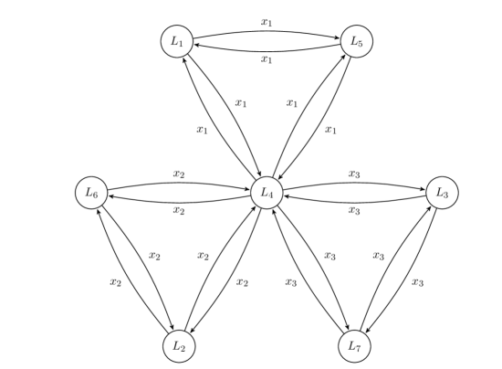
Figure 5: Each source-destination pair is displayed with the same color. We use $x_{i}$ to denote the flow corresponding to the $i^{th}$ source-destination pair and $L_{i}$ to denote the $i^{th}$ link. All 3 flows traverse link $L_{4}$.

Figure 6: Dual graph for the network in Figure 6, each link in this graph corresponds to the flows shared between the links in the original network. The node corresponding to link $L_{4}$ has high unweighted out-degree equal to $6$.

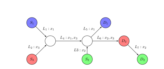
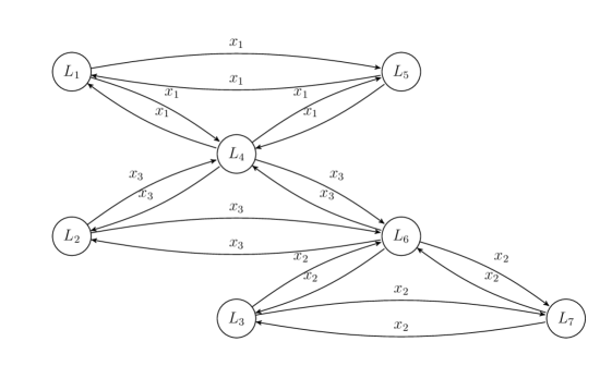
Figure 7: Each source-destination pair is displayed with the same color. We use $x_{i}$ to denote the flow corresponding to the $i^{th}$ source-destination pair and $L_{i}$ to denote the $i^{th}$ link. Each link has at most $2$ flows traversing it.

Figure 8: Dual graph for the network in Figure 8, each link in this graph corresponds to the flows shared between the links in the original network. Both nodes corresponding to links $L_{4}$ and $L_{6}$ has relatively high out-degree equal to $4$.

5.2 Convergence in Primal Iterations

We next present our convergence analysis for the primal sequence $\{x^{k}\}$ generated by the inexact Newton method (37). For the $k^{th}$ iteration, we define the function $\tilde{f}_{k}:\mathbb{R}\rightarrow\mathbb{R}$ as

$$\tilde{f}_{k}(t)=f(x^{k}+t\Delta\tilde{x}^{k}),$$ (52)

which is self-concordant, because the objective function $f$ is self-concordant. Note that the value $\tilde{f}_{k}(0)$ and $\tilde{f}_{k}(d^{k})$ are the objective function values at $x^{k}$ and $x^{k+1}$ respectively. Therefore $\tilde{f}_{k}(d^{k})-\tilde{f}_{k}(0)$ measures the decrease in the objective function value at the $k^{th}$ iteration. We will refer to the function $\tilde{f}_{k}$ as the objective function along the Newton direction.

Before proceeding further, we first introduce some properties of self-concordant functions and the Newton decrement, which will be used in our convergence analysis.

5.2.1 Preliminaries

Using the definition of a self-concordant function, we have the following result (see [9] for the proof).

Lemma 5.2.

Let $\tilde{f}:\mathbb{R}\rightarrow\mathbb{R}$ be a self-concordant function. Then for all $t\geq 0$ in the domain of the function $\tilde{f}$ with $t\tilde{f}^{\prime\prime}(0)^{\frac{1}{2}}<1$, the following inequality holds:

$$\tilde{f}(t)\leq\tilde{f}(0)+t\tilde{f}^{\prime}(0)-t{\tilde{f}}^{\prime\prime}(0)^{\frac{1}{2}}-\log(1-t\tilde{f}^{\prime\prime}(0)^{\frac{1}{2}}).$$ (53)

We will use the preceding lemma to prove a key relation in analyzing convergence properties of our algorithm [see Lemma 5.8]. The next lemma will be used to relate the weighted norms of a vector $z$, with weights $\nabla^{2}f(x)$ and $\nabla^{2}f(y)$ for some $x$ and $y$. This lemma plays an essential role in establishing properties for the Newton decrement (see [19], [30] for more details).

Lemma 5.3.

Let $f:\mathbb{R}^{n}\rightarrow\mathbb{R}$ be a self-concordant function. Suppose vectors $x$ and $y$ are in the domain of $f$ and $\tilde{\lambda}=((x-y)^{\prime}\nabla^{2}f(x)(x-y))^{\frac{1}{2}}<1$, then for any $z\in\mathbb{R}^{n}$, the following inequality holds:

$$(1-\tilde{\lambda})^{2}z^{\prime}\nabla^{2}f(x)z\leq z^{\prime}\nabla^{2}f(y)z\leq\frac{1}{(1-\tilde{\lambda})^{2}}z^{\prime}\nabla^{2}f(x)z.$$ (54)

The next two lemmas establish properties of the Newton decrement generated by the equality-constrained Newton method. The first lemma extends results in [19] and [30] to allow inexactness in the Newton direction and reflects the effect of the error in the current step on the Newton decrement in the next step.

Lemma 5.4.

Let $f:\mathbb{R}^{n}\to\mathbb{R}$ be a self-concordant function. Consider solving the equality constrained optimization problem

minimize $$f(x)$$ (55)

subject to $$Ax=c,$$

using an (exact) Newton method with feasible initialization, where the matrix $A$ is in $\mathbb{R}^{L\times(L+S)}$ and has full column rank, i.e., rank$(A)=L$. Let $\Delta x$ be the exact Newton direction at $x$, i.e., $\Delta x$ solves the following system of linear equations,

$$\left(\begin{array}[]{cc}\nabla^{2}f({x})&A^{\prime}\\ A&0\end{array}\right)\left(\begin{array}[]{c}\Delta x\\ w\end{array}\right)=-\left(\begin{array}[]{c}\nabla f({x})\\ 0\end{array}\right).$$ (62)

Let $\Delta\tilde{x}$ denote any direction with $\gamma=\Delta x-\Delta\tilde{x}$, and $x(t)=x+t\Delta\tilde{x}$ for $t\in[0,1]$. Let $z$ be the exact Newton direction at $x+\Delta\tilde{x}$. If $\tilde{\lambda}=\sqrt{\Delta\tilde{x}^{\prime}\nabla^{2}f(x)\Delta\tilde{x}}<1$, then we have

$$z\nabla^{2}f(x+\Delta\tilde{x})^{\prime}z \leq\frac{\tilde{\lambda}^{2}}{1-\tilde{\lambda}}\sqrt{z^{\prime}\nabla^{2}f(x)z}+|\gamma^{\prime}\nabla^{2}f(x)^{\prime}z|.$$

Proof.

We first transform problem (55) into an unconstrained one via elimination technique, establish equivalence in the Newton decrements and the Newton primal directions between the two problems following the lines in [9], then derive the results for the unconstrained problem and lastly we map the result back to the original constrained problem.

Since the matrix $A$ has full column rank, i.e., rank$(A)=L$, in order to eliminate the equality constraints, we let matrix $K\in\mathbb{R}^{(S+L)\times S}$ be any matrix whose range is null space of A, with rank$(K)=S$, vector $\hat{x}\in\mathbb{R}^{S+L}$ be a feasible solution for problem (55), i.e., $A\hat{x}=c$. Then we have the parametrization of the affine feasible set as

$$\{x|Ax=c\}=\{Ky+\hat{x}|y\in\mathbb{R}^{S}\}.$$

The eliminated equivalent optimization problem becomes

$$\mbox{minimize}_{y\in\mathbb{R}^{S}}\quad F(y)=f(Ky+\hat{x}).$$ (63)

We next show the Newton primal direction for the constrained problem (55) and unconstrained problem (63) are isomorphic, where a feasible solution $x$ for problem (55) is mapped to $y$ in problem (63) with $Ky+\hat{x}=x$. We start by showing that each $\Delta y$ in the unconstrained problem corresponds uniquely to the Newton direction in the constrained problem.

For the unconstrained problem, the gradient and Hessian are given by

$$\nabla F(y)=K^{\prime}\nabla f(Ky+\hat{x}),\quad\nabla^{2}F(y)=K^{\prime}\nabla^{2}f(Ky+\hat{x})K.$$ (64)

Note that the objective function $f$ is three times continuously differentiable, which implies its Hessian matrix $\nabla^{2}f(Ky+\hat{x})$ is symmetric, and therefore we have $\nabla^{2}F(y)$ is symmetric, i.e., $\nabla^{2}F(y)^{\prime}=\nabla^{2}F(y)$.

The Newton direction for problem (63) is given by

$$\Delta y=-\left(\nabla^{2}F(y)\right)^{-1}\nabla F(y)=-(K^{\prime}\nabla^{2}f(x)K)^{-1}K^{\prime}\nabla f(x).$$ (65)

We choose

$$w=-(AA^{\prime})^{-1}A(\nabla f(x)+\nabla^{2}f(x)\Delta x),$$ (66)

and show that $(\Delta x,w)$ where

$$\Delta x=K\Delta y$$ (67)

is the unique solution pair for the linear system (62) for the constrained problem (55). To establish the first equation, i.e., $\nabla^{2}f(x)\Delta x+A^{\prime}w=-\nabla f(x)$, we use the property that $\left(\begin{array}[]{c}K^{\prime}\\ A\end{array}\right)u=\left(\begin{array}[]{c}K^{\prime}u\\ Au\end{array}\right)=0$ for some $u\in\mathbb{R}^{S+L}$ implies $u=0$. We have

$$\left(\begin{array}[]{c}K^{\prime}\\ A\end{array}\right)\left(\begin{array}[]{c}\nabla^{2}f(x)\Delta x+A^{\prime}w+\nabla f(x)\end{array}\right)$$

$$= \left(\begin{array}[]{c}K^{\prime}\nabla^{2}f(x)K(-(K^{\prime}\nabla^{2}f(x)K)^{-1}K^{\prime}\nabla f(x))+K^{\prime}A^{\prime}w+K^{\prime}\nabla f(x)\\ A\nabla^{2}f(x)\Delta x-A(\nabla f(x)+\nabla^{2}f(x)\Delta x)+A\nabla f(x)\end{array}\right)$$

$$= \left(\begin{array}[]{c}0\\ 0\end{array}\right),$$

where the first equality follows from definition of $\Delta x$, $\Delta y$ and $w$ [cf. Eqs. (67), (65) and (66)] and the second equality follows the fact that $K^{\prime}A^{\prime}w=0$ for any $w$. Therefore we conclude that the first equation in (62) holds. Since the range of matrix $K$ is the null space of matrix $A$, we have $AKy=0$ for all $y$, therefore the second equation in (62) holds, i.e., $A\Delta x=0$.

For the converse, given a Newton direction $\Delta x$ defined as solution to the system (62) for the constrained problem (55), we can uniquely recover a vector $\Delta y$, such that $K\Delta y=\Delta x$. This is because $A\Delta x=0$ from (62), and hence $\Delta x$ is in the null space of the matrix $A$, i.e., column space of the matrix $K$. The matrix $K$ has full rank, thus there exists a unique $\Delta y$. Therefore the (primal) Newton directions for problems (63) and (55) are isomorphic under the mapping $K$. In what follows, we perform our analysis for the unconstrained problem (63) and then use isomorphic transformations to show the result hold for the equality constrained problem (55).

Consider the unconstrained problem (55), let $\Delta y$ denote the exact Newton direction at $y$ [cf. Eq. (64)], vector $\Delta\tilde{y}$ denote any direction in $\mathbb{R}^{S}$, $y(t)=y+t\Delta\tilde{y}$ and $\tilde{\lambda}=\sqrt{\Delta\tilde{y}^{\prime}\nabla^{2}F(y)\Delta\tilde{y}}$. Note that with the isomorphism established earlier, we have $\tilde{\lambda}=\sqrt{\Delta\tilde{y}^{\prime}\nabla^{2}F(y)\Delta\tilde{y}}=\sqrt{\Delta\tilde{y}^{\prime}K^{\prime}\nabla^{2}f(Ky+\hat{x})K\Delta\tilde{y}}=\sqrt{\Delta\tilde{x}^{\prime}\nabla^{2}f(x)\Delta\tilde{x}}$, where $x=Ky+\hat{x}$ and $\Delta\tilde{x}=K\Delta\tilde{y}$. From the assumption in the theorem, we have $\tilde{\lambda}<1$. For any $t<1$, $(y-y(t))^{\prime}\nabla^{2}F(y)(y-y(t))=t^{2}\tilde{\lambda}^{2}<1$ and by Lemma 5.3 for any $z_{y}$ in $\mathbb{R}^{S}$, we have

$$(1-t\tilde{\lambda})^{2}z_{y}^{\prime}\nabla^{2}F(y)z_{y}\leq z_{y}^{\prime}\nabla^{2}F(y(t))z_{y}\leq\frac{1}{(1-t\tilde{\lambda})^{2}}z_{y}^{\prime}\nabla^{2}F(y)z_{y}$$

which implies

$$z_{y}^{\prime}(\nabla^{2}F(y(t))-\nabla^{2}F(y))z_{y}\leq\left(\frac{1}{(1-t\tilde{\lambda})^{2}}-1\right)z_{y}^{\prime}\nabla^{2}F(y)z_{y},$$ (68)

and

$$z_{y}^{\prime}(\nabla^{2}F(y)-\nabla^{2}F(y(t)))z_{y}\leq\left(1-(1-t\tilde{\lambda})^{2}\right)z_{y}^{\prime}\nabla^{2}F(y)z_{y}.$$

Using the fact that $1-(1-t\tilde{\lambda})^{2}\leq\frac{1}{(1-t\tilde{\lambda})^{2}}-1$, the preceding relation can be rewritten as

$$z_{y}^{\prime}(\nabla^{2}F(y)-\nabla^{2}F(y(t)))z_{y}\leq\left(\frac{1}{(1-t\tilde{\lambda})^{2}}-1\right)z_{y}^{\prime}\nabla^{2}F(y)z_{y}.$$ (69)

Combining relations (68) and (69) yields

$$\left|z_{y}^{\prime}(\nabla^{2}F(y)-\nabla^{2}F(y(t)))z_{y}\right|\leq\left(\frac{1}{(1-t\tilde{\lambda})^{2}}-1\right)z_{y}^{\prime}\nabla^{2}F(y)z_{y}.$$ (70)

Since the function $F$ is convex, the Hessian matrix $\nabla^{2}F(y)$ is positive semidefinite. We can therefore apply the generalized Cauchy-Schwarz inequality and obtain

$$\left|(\Delta\tilde{y})^{\prime}(\nabla^{2}F(y(t))-\nabla^{2}F(y))z_{y}\right|$$ (71)

$$\leq\sqrt{(\Delta\tilde{y})^{\prime}(\nabla^{2}F(y(t))-\nabla^{2}F(y))\Delta\tilde{y}^{\prime}}\sqrt{z_{y}^{\prime}(\nabla^{2}F(y(t))-\nabla^{2}F(y))z_{y}}$$

$$\leq\left(\frac{1}{(1-t\tilde{\lambda})^{2}}-1\right)\sqrt{(\Delta\tilde{y})^{\prime}\nabla^{2}F(y)\Delta\tilde{y}}\sqrt{z_{y}^{\prime}\nabla^{2}F(y)z_{y}}$$

$$=\left(\frac{1}{(1-t\tilde{\lambda})^{2}}-1\right)\tilde{\lambda}\sqrt{z_{y}^{\prime}\nabla^{2}F(y)z_{y}},$$

where the second inequality follows from relation (70), and the equality follows from definition of $\tilde{\lambda}$.

Define the function $\kappa:\mathbb{R}\to\mathbb{R}$, as $\kappa(t)=\nabla F(y(t))^{\prime}z_{y}+(1-t)(\Delta\tilde{y})^{\prime}\nabla^{2}F(y)^{\prime}z_{y}$, then

$$\left|\frac{d}{dt}\kappa(t)\right|=\left|(\Delta\tilde{y})^{\prime}\nabla^{2}F(y(t))^{\prime}z_{y}-(\Delta\tilde{y})^{\prime}\nabla^{2}F(y)z_{y}\right|=\left|(\Delta\tilde{y})^{\prime}(\nabla^{2}F(y(t))-\nabla^{2}F(y))z_{y}\right|,$$

which is the left hand side of (71).

Define $\gamma_{y}=\Delta y-\Delta\tilde{y}$, which by the isomorphism, implies $\gamma=\Delta x-\Delta\tilde{x}=K\gamma_{y}$. By rewriting $\Delta\tilde{y}=\Delta y-\gamma_{y}$ and observing the exact Newton direction $\Delta y$ satisfies $\Delta y=-\nabla^{2}F(y)^{-1}\nabla F(y)$ [cf. Eq. (64)] and hence by symmetry of the matrix $\nabla^{2}F(y)$, we have $\Delta y^{\prime}\nabla^{2}F(y)=\Delta y^{\prime}\nabla^{2}F(y)^{\prime}=-\nabla F(y)^{\prime}$, we obtain

$$\kappa(0)=\nabla F(y)^{\prime}z_{y}+(\Delta\tilde{y})^{\prime}\nabla^{2}F(y)^{\prime}z_{y}=\nabla F(y)^{\prime}z_{y}-\nabla F(y)^{\prime}z_{y}-\gamma_{y}^{\prime}\nabla^{2}F(y)z_{y}=-\gamma_{y}^{\prime}\nabla^{2}F(y)z_{y}.$$

Hence by integration, we obtain the bound

$$\left|\kappa(t)\right| \leq\tilde{\lambda}\sqrt{z_{y}^{\prime}\nabla^{2}F(y)z_{y}}{\int}_{0}^{t}\left(\frac{1}{(1-s\tilde{\lambda})^{2}}-1\right)ds+|\gamma_{y}^{\prime}\nabla^{2}F(y)z_{y}|$$

$$=\frac{\tilde{\lambda}^{2}t^{2}}{1-\tilde{\lambda}t}\sqrt{z_{y}^{\prime}\nabla^{2}F(y)z_{y}}+|\gamma_{y}^{\prime}\nabla^{2}F(y)z_{y}|.$$

For $t=1$, $y(t)=y+\Delta\tilde{y}$, above equation implies

$$\left|\kappa(1)\right| =\left|\nabla F(y+\Delta\tilde{y})^{\prime}z_{y}\right| \leq\frac{\tilde{\lambda}^{2}}{1-\tilde{\lambda}}\sqrt{z_{y}^{\prime}\nabla^{2}F(y)z_{y}}+|\gamma_{y}^{\prime}\nabla^{2}F(y)z_{y}|.$$

We now specify $z_{y}$ to be the exact Newton direction at $y+\Delta\tilde{y}$, then $z_{y}$ satisfies $z_{y}^{\prime}\nabla^{2}F(y+\Delta\tilde{y})z_{y}=\left|\nabla F(y+\Delta\tilde{y})^{\prime}z_{y}\right|$, by using the definition of Newton direction at $y+\Delta\tilde{y}$ [cf. Eq. (65)], which proves

$$z_{y}\nabla^{2}F(y+\Delta\tilde{y})z_{y} \leq\frac{\tilde{\lambda}^{2}}{1-\tilde{\lambda}}\sqrt{z_{y}^{\prime}\nabla^{2}F(y)z_{y}}+|\gamma_{y}^{\prime}\nabla^{2}F(y)^{\prime}z_{y}|.$$

We now use the isomorphism once more to transform the above relation to the equality constrained problem domain. We have $z=Kz_{y}$, the exact Newton direction at $x+\Delta\tilde{x}=\hat{x}+Ky+K\Delta\tilde{y}$. The left hand side becomes

$$z_{y}^{\prime}\nabla^{2}F(y+\Delta\tilde{y})z_{y}=z_{y}^{\prime}K^{\prime}\nabla^{2}f(x+\Delta\tilde{x})Kz_{y}=z^{\prime}\nabla^{2}f(x+\Delta\tilde{x})z.$$

Similarly, we have the right hand sand satisfies

$$\frac{\tilde{\lambda}^{2}}{1-\tilde{\lambda}}\sqrt{z_{y}^{\prime}\nabla^{2}F(y)z_{y}}+|\gamma_{y}^{\prime}\nabla^{2}F(y)^{\prime}z_{y}| =\frac{\tilde{\lambda}^{2}}{1-\tilde{\lambda}}\sqrt{z_{y}^{\prime}K^{\prime}\nabla^{2}f(x)Kz_{y}}+|\gamma_{y}^{\prime}K^{\prime}\nabla^{2}f(x)Kz_{y}|$$

$$=\frac{\tilde{\lambda}^{2}}{1-\tilde{\lambda}}\sqrt{z^{\prime}\nabla^{2}f(x)z}+|\gamma^{\prime}\nabla^{2}f(x)^{\prime}z|.$$

By combining the above two relations, we have established the desired relation. ∎

One possible matrix $K$ in the above proof for problem (4) is given by $K=\left(\begin{array}[]{c}I(S)\\ -R\end{array}\right)$, whose corresponding unconstrained domain consists of the source rate variables. In the unconstrained domain, the source rates are updated and then the matrix $K$ adjusts the slack variables accordingly to maintain the feasibility, which coincides with our inexact distributed algorithm in the primal domain. The above lemma will be used to guarantee quadratic rate of convergence for the distributed inexact Newton method (37)]. The next lemma plays a central role in relating the suboptimality gap in the objective function value to the exact Newton decrement (see [9] for more details).

Lemma 5.5.

Let $F:\mathbb{R}^{n}\to\mathbb{R}$ be a self-concordant function. Consider solving the unconstrained optimization problem

$$\hbox{minimize}_{x\in\mathbb{R}^{n}}\ F(x),$$ (72)

using an (unconstrained) Newton method. Let $\Delta x$ be the exact Newton direction at $x$, i.e., $\Delta x=-\nabla^{2}F(x)^{-1}\nabla F(x)$. Let $\lambda(x)$ be the exact Newton decrement, i.e., $\lambda(x)=\sqrt{(\Delta{x})^{\prime}\nabla^{2}F(x)\Delta{x}}$. Let $F^{*}$ denote the optimal value of problem (72). If $\lambda(x)\leq 0.68$, then we have

$$F^{*}\geq F(x)-\lambda(x)^{2}.$$ (73)

Using the same elimination technique and isomorphism established for Lemma 5.4, the next result follows immediately.

Lemma 5.6.

Let $f:\mathbb{R}^{n}\to\mathbb{R}$ be a self-concordant function. Consider solving the equality constrained optimization problem

minimize $$f(x)$$ (74)

subject to $$Ax=c,$$

using a constrained Newton method with feasible initialization. Let $\Delta x$ be the exact (primal) Newton direction at $x$, i.e., $\Delta x$ solves the system

$$\left(\begin{array}[]{cc}\nabla^{2}f({x})&A^{\prime}\\ A&0\end{array}\right)\left(\begin{array}[]{c}\Delta x\\ w\end{array}\right)=-\left(\begin{array}[]{c}\nabla f({x})\\ 0\end{array}\right).$$

Let $\lambda(x)$ be the exact Newton decrement, i.e., $\lambda(x)=\sqrt{(\Delta{x})^{\prime}\nabla^{2}f(x)\Delta{x}}$. Let $f^{*}$ denote the optimal value of problem (74). If $\lambda(x)\leq 0.68$, then we have

$$f^{*}\geq f(x)-\lambda(x)^{2}.$$ (75)

Note that the relation on the suboptimality gap in the preceding lemma holds when the exact Newton decrement is sufficiently small (provided by the numerical bound 0.68, see [9]). We will use these lemmas in the subsequent sections for the convergence rate analysis of the distributed inexact Newton method applied to problem (4). Our analysis comprises of two parts: The first part is the damped convergent phase, in which we provide a lower bound on the improvement in the objective function value at each step by a constant. The second part is the quadratically convergent phase, in which the suboptimality in the objective function value diminishes quadratically to an error level.

5.2.2 Basic Relations

We first introduce some key relations, which provides a bound on the error in the Newton direction computation. This will be used for both phases of the convergence analysis.

Lemma 5.7.

Let $\{x^{k}\}$ be the primal sequence generated by the inexact Newton method (37). Let $\tilde{\lambda}(x^{k})$ be the inexact Newton decrement at $x^{k}$ [cf. Eq. (39)]. For all $k$, we have

$$|(\gamma^{k})^{\prime}\nabla^{2}f(x^{k})\Delta\tilde{x}^{k}|\leq p\tilde{\lambda}(x^{k})^{2}+\tilde{\lambda}(x^{k})\sqrt{\epsilon},$$

where $\gamma^{k}$, $p$, and $\epsilon$ are nonnegative scalars defined in Assumption 2.

Proof.

By Assumption 1, the Hessian matrix $\nabla^{2}f(x^{k})$ is positive definite for all $x^{k}$. We therefore can apply the generalized Cauchy-Schwarz inequality and obtain

$$|(\gamma^{k})^{\prime}\nabla^{2}f(x^{k})\Delta\tilde{x}^{k}| \leq\sqrt{((\gamma^{k})^{\prime}\nabla^{2}f(x^{k})\gamma^{k})((\Delta\tilde{x}^{k})^{\prime}\nabla^{2}f(x^{k})\Delta\tilde{x}^{k})}$$ (76)

$$\leq\sqrt{(p^{2}\tilde{\lambda}(x^{k})^{2}+\epsilon)\tilde{\lambda}(x^{k})^{2}}$$

$$\leq\sqrt{(p^{2}\tilde{\lambda}(x^{k})^{2}+\epsilon+2p\tilde{\lambda}(x^{k})\sqrt{\epsilon})\tilde{\lambda}(x^{k})^{2}},$$

where the second inequality follows from Assumption 2 and definition of $\tilde{\lambda}(x^{k})$, and the third inequality follows by adding the nonnegative term $2p\sqrt{\epsilon}\tilde{\lambda}(x^{k})^{3}$ to the right hand side. By the nonnegativity of the inexact Newton decrement $\tilde{\lambda}(x^{k})$, it can be seen that relation (76) implies

$$|(\gamma^{k})^{\prime}\nabla^{2}f(x^{k})\Delta\tilde{x}^{k}|\leq\tilde{\lambda}(x^{k})(p\tilde{\lambda}(x^{k})+\sqrt{\epsilon})=p\tilde{\lambda}(x^{k})^{2}+\tilde{\lambda}(x^{k})\sqrt{\epsilon},$$

which proves the desired relation. ∎

Using the preceding lemma, the following basic relation can be established, which will be used to measure the improvement in the objective function value.

Lemma 5.8.

Let $\{x^{k}\}$ be the primal sequence generated by the inexact Newton method (37). Let $\tilde{f}_{k}$ be the objective function along the Newton direction and $\tilde{\lambda}(x^{k})$ be the inexact Newton decrement [cf. Eqs. (52) and (39)] at $x^{k}$ respectively. For all $k$ with $0\leq t<1/{\tilde{\lambda}(x^{k})}$, we have

$$\tilde{f}_{k}(t)\leq\tilde{f}_{k}(0)-t(1-p)\tilde{\lambda}(x^{k})^{2}-(1-\sqrt{\epsilon})t\tilde{\lambda}(x^{k})-\log(1-t\tilde{\lambda}(x^{k})),$$ (77)

where $p$, and $\epsilon$ are the nonnegative scalars defined in Assumption 2.

Proof.

Recall that $\Delta x^{k}$ is the exact Newton direction, which solves the system (15). Therefore for some $w^{k}$, the following equation is satisfied,

$$\nabla^{2}f(x^{k})\Delta x^{k}+A^{\prime}w^{k}=-\nabla f(x^{k}).$$

By left multiplying the above relation by $(\Delta\tilde{x}^{k})^{\prime}$, we obtain

$$(\Delta\tilde{x}^{k})^{\prime}\nabla^{2}f(x^{k})\Delta x^{k}+(\Delta\tilde{x}^{k})^{\prime}A^{\prime}w^{k}=-(\Delta\tilde{x}^{k})^{\prime}\nabla f(x^{k}).\\$$

Using the facts that $\Delta x^{k}=\Delta\tilde{x}^{k}+\gamma^{k}$ from Assumption 2 and $A\Delta\tilde{x}^{k}=0$ by the design of our algorithm, the above relation yields

$$(\Delta\tilde{x}^{k})^{\prime}\nabla^{2}f(x)\Delta\tilde{x}^{k}+(\Delta\tilde{x}^{k})^{\prime}\nabla^{2}f(x^{k})\gamma^{k}=-(\Delta\tilde{x}^{k})^{\prime}\nabla f(x^{k}).$$

By Lemma 5.7, we can bound $(\Delta\tilde{x}^{k})^{\prime}\nabla^{2}f(x^{k})\gamma^{k}$ by,

$$p\tilde{\lambda}(x^{k})^{2}+\tilde{\lambda}(x^{k})\sqrt{\epsilon}\geq(\Delta\tilde{x}^{k})^{\prime}\nabla^{2}f(x^{k})\gamma^{k}\geq-p\tilde{\lambda}(x^{k})^{2}-\tilde{\lambda}(x^{k})\sqrt{\epsilon}.$$

Using the definition of $\tilde{\lambda}(x^{k})$ [cf. Eq. (39)] and the preceding two relations, we obtain the following bounds on $(\Delta\tilde{x}^{k})^{\prime}\nabla f(x^{k})$:

$$-(1+p)\tilde{\lambda}(x^{k})^{2}-\tilde{\lambda}(x^{k})\sqrt{\epsilon}\leq(\Delta\tilde{x}^{k})^{\prime}\nabla f(x^{k})\leq-(1-p)\tilde{\lambda}(x^{k})^{2}+\tilde{\lambda}(x^{k})\sqrt{\epsilon}.$$

By differentiating the function $\tilde{f_{k}}(t)$, and using the preceding relation, this yields,

$$\tilde{f}_{k}^{\prime}(0) =\nabla f(x^{k})^{\prime}\Delta\tilde{x}^{k}$$ (78)

$$\leq-(1-p)\tilde{\lambda}(x^{k})^{2}+\tilde{\lambda}(x^{k})\sqrt{\epsilon}.$$

Moreover, we have

$$\tilde{f}_{k}^{\prime\prime}(0) =(\Delta\tilde{x}^{k})^{\prime}\nabla^{2}f(x^{k})\Delta\tilde{x}^{k}$$ (79)

$$=\tilde{\lambda}(x^{k})^{2}.$$

The function $\tilde{f}_{k}(t)$ is self-concordant for all $k$, therefore by Lemma 5.2, for $0\leq t<1/{\tilde{\lambda}(x^{k})}$, the following relations hold:

$$\tilde{f}_{k}(t) \leq\tilde{f}_{k}(0)+t\tilde{f}_{k}^{\prime}(0)-t\tilde{f}_{k}^{\prime\prime}(0)^{\frac{1}{2}}-\log(1-tf_{k}^{\prime\prime}(0)^{\frac{1}{2}})$$

$$\leq\tilde{f}_{k}(0)-t(1-p)\tilde{\lambda}(x^{k})^{2}+t\tilde{\lambda}(x^{k})\sqrt{\epsilon}-t\tilde{\lambda}(x^{k})-\log(1-t\tilde{\lambda}(x^{k}))$$

$$=\tilde{f}_{k}(0)-t(1-p)\tilde{\lambda}(x^{k})^{2}-(1-\sqrt{\epsilon})t\tilde{\lambda}(x^{k})-\log(1-t\tilde{\lambda}(x^{k})),$$

where the second inequality follows by Eqs. (78) and (79). This proves Eq. (77). ∎

The preceding lemma shows that a careful choice of the stepsize $t$ can guarantee a constant lower bound on the improvement in the objective function value at each iteration. We present the convergence properties of our algorithm in the following two sections.

5.2.3 Damped Convergent Phase

In this section, we consider the case when $\theta^{k}\geq V$ and stepsize $d^{k}=\frac{b}{\theta^{k}+1}$ [cf. Eq. (42)]. We will provide a constant lower bound on the improvement in the objective function value in this case. To this end, we first establish the improvement bound for the exact stepsize choice of $t=1/(\tilde{\lambda}(x^{k})+1)$.

Theorem 5.9.

Let $\{x^{k}\}$ be the primal sequence generated by the inexact Newton method (37). Let $\tilde{f}_{k}$ be the objective function along the Newton direction and $\tilde{\lambda}(x^{k})$ be the inexact Newton decrement at $x^{k}$ [cf. Eqs. (52) and (39)]. Consider the scalars $p$ and $\epsilon$ defined in Assumption 2 and assume that $0<p<\frac{1}{2}$ and $0<\epsilon<\left(\frac{\left(0.5-p\right)(2Vb-V+b-1)}{b}\right)^{2}$, where $b$ is the constant used in the stepsize rule [cf. Eq. (42)]. For $\theta^{k}\geq V$ and $t=1/\left(\tilde{\lambda}(x^{k})+1\right)$, there exists a scalar $\alpha>0$ such that

$$\tilde{f}_{k}(t)-\tilde{f}_{k}(0) \leq-\alpha\left(1+p\right)\left(\frac{2Vb-V+b-1}{b}\right)^{2}\Big{/}\left(1+\frac{2Vb-V+b-1}{b}\right).$$ (80)

Proof.

For notational simplicity, let $y=\tilde{\lambda}\left(x^{k}\right)$ in this proof. We will show that for any positive scalar $\alpha$ with $0<\alpha\leq\left(\frac{1}{2}-p-\frac{\sqrt{\epsilon}b}{(2Vb-V+b-1)}\right)/\left(p+1\right)$, Eq. (80) holds. Note that such $\alpha$ exists since $\epsilon<\left(\frac{\left(0.5-p\right)(2Vb-V+b-1)}{b}\right)^{2}$.

By Assumption 3, we have for $\theta^{k}\geq V$,

$$y\geq\theta^{k}-\left(\frac{1}{b}-1\right)(1+V)\geq V-\left(\frac{1}{b}-1\right)(1+V)=\frac{2Vb-V+b-1}{b}.$$ (81)

Using $b>\frac{V+1}{2V+1}$, we have $y\geq V-\left(\frac{1}{b}-1\right)(1+V)>0$, which implies $2Vb-V+b-1>0$. Together with $0<\alpha\leq\left(\frac{1}{2}-p-\frac{\sqrt{\epsilon}b}{2Vb-V+b-1}\right)/\left(p+1\right)$ and $b>\frac{V+1}{2V+1}$, this shows

$$\sqrt{\epsilon}\leq\frac{2Vb-V+b-1}{b}\left(\frac{1}{2}-p-\alpha\left(1+p\right)\right).$$

Combining the above, we obtain

$$\sqrt{\epsilon}\leq y\left(\frac{1}{2}-p-\alpha\left(1+p\right)\right),$$

which using algebraic manipulation yields

$$-\left(1-p\right)y-\left(1-\sqrt{\epsilon}\right)+\left(1+y\right)-\frac{y}{2}\leq-\alpha\left(1+p\right)y.$$

From Eq. (81), we have $y>0$. We can therefore multiply by $y$ and divide by $1+y$ both sides of the above inequality to obtain

$$-\frac{1-p}{1+y}y^{2}-\frac{1-\sqrt{\epsilon}}{1+y}y+y-\frac{y^{2}}{2\left(1+y\right)}\leq-\alpha\frac{\left(1+p\right)y^{2}}{1+y}$$ (82)

Using second order Taylor expansion on $\log\left(1+y\right)$, we have for $y\geq 0$

$$\log\left(1+y\right)\leq y-\frac{y^{2}}{2\left(1+y\right)}.$$

Using this relation in Eq. (82) yields,

$$-\frac{1-p}{1+y}y^{2}-\frac{1-\sqrt{\epsilon}}{1+y}y+\log\left(1+y\right)\leq-\alpha\frac{\left(1+p\right)y^{2}}{1+y}.$$

Substituting the value of $t=1/\left(y+1\right)$, the above relation can be rewritten as

$$-\left(1-p\right)ty^{2}-\left(1-\sqrt{\epsilon}\right)ty-\log\left(1-ty\right)\leq-\alpha\frac{\left(1+p\right)y^{2}}{1+y}.$$

Using Eq. (77) from Lemma 5.8 and definition of $y$ in the preceding, we obtain

$$\tilde{f}_{k}\left(t\right)-\tilde{f}_{k}\left(0\right)\leq-\alpha\left(1+p\right)\frac{y^{2}}{y+1}.$$

Observe that the function $h\left(y\right)=\frac{y^{2}}{y+1}$ is monotonically increasing in $y$, and for $\theta^{k}\geq V$ by relation (81) we have $y\geq\frac{2Vb-V+b-1}{b}$. Therefore

$$-\alpha\left(1+p\right)\frac{y^{2}}{y+1}\leq-\alpha\left(1+p\right)\left(\frac{2Vb-V+b-1}{b}\right)^{2}/\left(1+\frac{2Vb-V+b-1}{b}\right).$$

Combining the preceding two relations completes the proof. ∎

Note that our algorithm uses the stepsize $d^{k}=\frac{d}{\theta^{k}+1}$ in the damped convergent phase, which is an approximation to the stepsize $t=1/(\tilde{\lambda}(x^{k})+1)$ used in the previous theorem. The error between the two is bounded by relation (46) as shown in Lemma 4.5. We next show that with this error in the stepsize computation, the improvement in the objective function value in the inexact algorithm is still lower bounded at each iteration.

Let $\beta=\frac{d^{k}}{t}$, where $t=1/(\tilde{\lambda}(x^{k})+1)$. By the convexity of $f$, we have

$$f(x^{k}+\beta t\Delta x^{k})=f(\beta(x^{k}+t\Delta x^{k})+(1-\beta)(x^{k}))\leq\beta f(x^{k}+t\Delta x^{k})+(1-\beta)f(x^{k}).$$

Therefore the objective function value improvement is bounded by

$$f(x+\beta t\Delta x^{k})-f(x^{k}) \leq\beta f(x^{k}+t\Delta x^{k})+(1-\beta)f(x^{k})-f(x^{k})$$

$$=\beta(f(x^{k}+t\Delta x^{k})-f(x^{k}))$$

$$=\beta(\tilde{f}_{k}(t)-\tilde{f}_{k}(0)),$$

where the last equality follows from the definition of $\tilde{f}_{k}(t)$. Using Lemma 4.5, we obtain bounds on $\beta$ as $2b-1\leq\beta\leq 1$. Hence combining this bound with Theorem 5.9, we obtain

$$f(x^{k+1})-f(x^{k})\leq-(2b-1)\alpha\left(1+p\right)\frac{\left(\frac{2Vb-V+b-1}{b}\right)^{2}}{\left(1+\frac{2Vb-V+b-1}{b}\right)}.$$ (83)

Hence in the damped convergent phase we can guarantee a lower bound on the object function value improvement at each iteration. This bound is monotone in $b$, i.e., the closer the scalar $b$ is to $1$, the faster the objective function value improves, however this also requires the error in the inexact Newton decrement calculation, i.e., $\tilde{\lambda}(x^{k})-\theta^{k}$, to diminish to $0$ [cf. Assumption 3].

5.2.4 Quadratically Convergent Phase

In this phase, there exists $\bar{k}$ with $\theta^{\bar{k}}<V$ and the step size choice is $d^{k}=1$ for all $k\geq\bar{k}$. We show that the suboptimality in the primal objective function value diminishes quadratically to a neighborhood of optimal solution. We proceed by first establishing the following lemma for relating the exact and the inexact Newton decrements.

Lemma 5.10.

Let $\{x^{k}\}$ be the primal sequence generated by the inexact Newton method (37) and $\lambda(x^{k})$, $\tilde{\lambda}(x^{k})$ be the exact and inexact Newton decrements at $x^{k}$ [cf. Eqs. (38) and (39)]. Let $p$ and $\epsilon$ be the nonnegative scalars defined in Assumption 2. We have

$$(1-p)\tilde{\lambda}(x^{k})-\sqrt{\epsilon}\leq\lambda(x^{k})\leq(1+p)\tilde{\lambda}(x^{k})+\sqrt{\epsilon}.$$ (84)

Proof.

By Assumption 1, for all $k$, $\nabla^{2}f(x^{k})$ is positive definite. We therefore can apply the generalized Cauchy-Schwarz inequality and obtain

$$|(\Delta x^{k})^{\prime}\nabla^{2}f(x^{k})\Delta\tilde{x}^{k}| \leq\sqrt{((\Delta{x^{k}})^{\prime}\nabla^{2}f(x^{k})\Delta x^{k})((\Delta\tilde{x}^{k})^{\prime}\nabla^{2}f(x^{k})\Delta\tilde{x}^{k})}$$ (85)

$$=\lambda(x^{k})\tilde{\lambda}(x^{k}),$$

where the equality follows from definition of $\lambda(x^{k})$ and $\tilde{\lambda}(x^{k})$. Note that by Assumption 2, we have $\Delta x^{k}=\Delta\tilde{x}^{k}+\gamma^{k}$, and hence

$$|(\Delta x^{k})^{\prime}\nabla^{2}f(x^{k})\Delta\tilde{x}^{k}| =|(\Delta\tilde{x}^{k}+\gamma^{k})^{\prime}\nabla^{2}f(x^{k})\Delta\tilde{x}^{k}|$$ (86)

$$\geq(\Delta\tilde{x}^{k})^{\prime}\nabla^{2}f(x^{k})\Delta\tilde{x}^{k}-|(\gamma^{k})^{\prime}\nabla^{2}f(x^{k})\Delta\tilde{x}^{k}|$$

$$\geq\tilde{\lambda}(x^{k})^{2}-p\tilde{\lambda}(x^{k})^{2}-\tilde{\lambda}(x^{k})\sqrt{\epsilon},$$

where the first inequality follows from a variation of triangle inequality, and the last inequality follows from Lemma 5.8. Combining the two inequalities (85) and (86), we obtain

$$\lambda(x^{k})\tilde{\lambda}(x^{k})\geq\tilde{\lambda}(x^{k})^{2}-p\tilde{\lambda}(x^{k})^{2}-\sqrt{\epsilon}\tilde{\lambda}(x^{k}),$$

By canceling the nonnegative term $\tilde{\lambda}(x^{k})$ on both sides, we have

$$\lambda(x^{k})\geq\tilde{\lambda}(x^{k})-p\tilde{\lambda}(x^{k})-\sqrt{\epsilon}.$$

This shows the first half of the relation (84). For the second half, using the definition of $\lambda(x^{k})$, we have

$$\lambda(x^{k})^{2} =(\Delta x^{k})^{\prime}\nabla^{2}f(x^{k})\Delta x^{k}$$

$$=(\Delta\tilde{x}^{k}+\gamma^{k})^{\prime}\nabla^{2}f(x^{k})(\Delta\tilde{x}^{k}+\gamma^{k})$$

$$=(\Delta\tilde{x}^{k})^{\prime}\nabla^{2}f(x^{k})\Delta\tilde{x}^{k}+(\gamma^{k})^{\prime}\nabla^{2}f(x^{k})\gamma^{k}+2(\Delta\tilde{x}^{k})^{\prime}\nabla^{2}f(x^{k})\gamma^{k},$$

where the second equality follows from the definition of $\gamma^{k}$ [cf. Eq. (43)]. By using the definition of $\tilde{\lambda}(x^{k})$, Assumption 2 and Lemma 5.7, the preceding relation implies,

$$\lambda(x^{k})^{2} \leq\tilde{\lambda}(x^{k})^{2}+p^{2}\tilde{\lambda}(x^{k})^{2}+\epsilon+2p\tilde{\lambda}(x^{k})^{2}+2\sqrt{\epsilon}\tilde{\lambda}(x^{k})$$

$$\leq\tilde{\lambda}(x^{k})^{2}+p^{2}\tilde{\lambda}(x^{k})^{2}+2p\tilde{\lambda}(x^{k})^{2}+2\sqrt{\epsilon}(1+p)\tilde{\lambda}(x^{k})+\epsilon$$

$$=((1+p)\tilde{\lambda}(x^{k})+\sqrt{\epsilon})^{2},$$

where the second inequality follows by adding a nonnegative term of $2\sqrt{\epsilon}p\tilde{\lambda}(x^{k})$ to the right hand side. By nonnegativity of $p$, $\epsilon$, $\lambda$ and $\tilde{\lambda}(x^{k})$, we can take the square root of both sides and this completes the proof for relation (84). ∎

Before proceeding to establish quadratic convergence in terms of the primal iterations to an error neighborhood of the optimal solution, we need to impose the following bound on the errors in our algorithm in this phase. Recall that $\bar{k}$ is an index such that $\theta^{\bar{k}}<V$ and $d^{k}=1$ for all $k\geq\bar{k}$.

Assumption 4.

Let $\{x^{k}\}$ be the primal sequence generated by the inexact Newton method (37). Let $\phi$ be a positive scalar with $\phi\leq 0.267$. Let $\xi$ and $v$ be nonnegative scalars defined in terms of $\phi$ as

$$\xi=\frac{\phi p+\sqrt{\epsilon}}{1-p-\phi-\sqrt{\epsilon}}+\frac{2\phi\sqrt{\epsilon}+\epsilon}{(1-p-\phi-\sqrt{\epsilon})^{2}},\quad\quad v=\frac{1}{(1-p-\phi-\sqrt{\epsilon})^{2}},$$

where $p$ and $\epsilon$ are the scalars defined in Assumption 2. The following relations hold

$$(1+p)(\theta^{\bar{k}}+\tau^{\bar{k}})+\sqrt{\epsilon}\leq\phi,$$ (87)

$$v(0.68)^{2}+\xi\leq 0.68,$$ (88)

$$\frac{0.68+\sqrt{\epsilon}}{1-p}\leq 1,$$ (89)

$$p+\sqrt{\epsilon}\leq 1-(4\phi^{2})^{\frac{1}{4}}-\phi,$$ (90)

where $\tau^{\bar{k}}>0$ is a bound on the error in the Newton decrement calculation at step $\bar{k}$ [cf. Assumption 3].

The upper bound of $0.267$ on $\phi$ is necessary here to guarantee relation (90) can be satisfied by some nonnegative scalars $p$ and $\epsilon$. Relation (87) can be satisfied by some nonnegative scalars $p$, $\epsilon$ and $\tau^{\bar{k}}$, because we have $\theta^{\bar{k}}<V<0.267$. Relation (87) and (88) will be used to guarantee the condition $\lambda(x^{k})\leq 0.68$ is satisfied throughout this phase, so that we can use Lemma 5.6 to relate the suboptimality bound with the Newton decrement, and relation (89) and (90) will be used for establishing the quadratic rate of convergence of the objective function value, as we will show in the Theorem 5.12. This assumption can be satisfied by first choosing proper values for the scalars $p$, $\epsilon$ and $\tau$ such that all the relations are satisfied, and then adapt both the consensus algorithm for $\theta^{\bar{k}}$ and the dual iterations for $w^{k}$ according to the desired precision (see the discussions following Assumption 2 and 3 for how these precision levels can be achieved).

To show the quadratic rate of convergence for the primal iterations, we need the following lemma, which relates the exact Newton decrement at the current and the next step.

Lemma 5.11.

Let $\{x^{k}\}$ be the primal sequence generated by the inexact Newton method (37) and $\lambda(x^{k})$, $\tilde{\lambda}(x^{k})$ be the exact and inexact Newton decrements at $x^{k}$ [cf. Eqs. (38) and (39)]. Let $\theta^{k}$ be the computed inexact value of $\tilde{\lambda}(x^{k})$ and let Assumption 4 hold. Then for all $k$ with $\tilde{\lambda}(x^{k})<1$, we have

$$\lambda(x^{k+1})\leq v\lambda(x^{k})^{2}+\xi,$$ (91)

where $\xi$ and $v$ are the scalars defined in Assumption 4 and $p$ and $\epsilon$ are defined as in Assumption 2.

Proof.

Given $\tilde{\lambda}(x^{k})<1$, we can apply Lemma 5.4 by letting $z=\Delta x^{k+1}$, we have

$$\lambda(x^{k+1})^{2} =(\Delta x^{k+1})^{\prime}\nabla f^{2}(x+\Delta\tilde{x})\Delta x^{k+1}$$

$$\leq\frac{\tilde{\lambda}(x^{k})^{2}}{1-\tilde{\lambda}(x^{k})}\sqrt{(\Delta x^{k+1})^{\prime}\nabla^{2}f(x)\Delta x^{k+1}}+\left|(\gamma^{k})^{\prime}\nabla^{2}f(x)^{\prime}\Delta x^{k+1}\right|$$

$$\leq\frac{\tilde{\lambda}(x^{k})^{2}}{1-\tilde{\lambda}(x^{k})}\sqrt{(\Delta x^{k+1})^{\prime}\nabla^{2}f(x)\Delta x^{k+1}}+\sqrt{(\gamma^{k})^{\prime}\nabla^{2}f(x)\gamma^{k}}\sqrt{(\Delta x^{k+1})^{\prime}\nabla^{2}f(x)\Delta x^{k+1}},$$

where the last inequality follows from the generalized Cauchy-Schwarz inequality. Using Assumption 2, the above relation implies

$$\lambda(x^{k+1})^{2} \leq\left(\frac{\tilde{\lambda}(x^{k})^{2}}{1-\tilde{\lambda}(x^{k})}+\sqrt{p^{2}\tilde{\lambda}(x^{k})^{2}+\epsilon}\right)\sqrt{(\Delta x^{k+1})^{\prime}\nabla^{2}f(x)\Delta x^{k+1}}.$$

By the fact that $\tilde{\lambda}(x^{k})\leq\theta^{k}+\tau\leq\phi<1$, we can apply Lemma 5.3 and obtain,

$$\lambda(x^{k+1})^{2} \leq\frac{1}{1-\tilde{\lambda}(x^{k})}\left(\frac{\tilde{\lambda}(x^{k})^{2}}{1-\tilde{\lambda}(x^{k})}+\sqrt{p^{2}\tilde{\lambda}(x^{k})^{2}+\epsilon}\right)\sqrt{(\Delta x^{k+1})^{\prime}\nabla^{2}f(x+\Delta\tilde{x})\Delta x^{k+1}}$$

$$=\left(\frac{\tilde{\lambda}(x^{k})^{2}}{(1-\tilde{\lambda}(x^{k}))^{2}}+\frac{\sqrt{p^{2}\tilde{\lambda}(x^{k})^{2}+\epsilon}}{1-\tilde{\lambda}(x^{k})}\right)\lambda(x^{k+1}).$$

By dividing the last line by $\lambda(x^{k+1})$, this yields

$$\lambda(x^{k+1})\leq\frac{\tilde{\lambda}(x^{k})^{2}}{(1-\tilde{\lambda}(x^{k}))^{2}}+\frac{\sqrt{p^{2}\tilde{\lambda}(x^{k})^{2}+\epsilon}}{1-\tilde{\lambda}(x^{k})}\leq\frac{\tilde{\lambda}(x^{k})^{2}}{(1-\tilde{\lambda}(x^{k}))^{2}}+\frac{p\tilde{\lambda}(x^{k})+\sqrt{\epsilon}}{1-\tilde{\lambda}(x^{k})}.$$

From Eq. (84), we have $\tilde{\lambda}(x^{k})\leq\frac{\lambda(x^{k})+\sqrt{\epsilon}}{1-p}$. Therefore the above relation implies

$$\lambda(x^{k+1})\leq\left(\frac{\lambda(x^{k})+\sqrt{\epsilon}}{1-p-\lambda(x^{k})-\sqrt{\epsilon}}\right)^{2}+\frac{p\lambda(x^{k})+\sqrt{\epsilon}}{1-p-\lambda(x^{k})-\sqrt{\epsilon}}.$$

By Eq. (93), we have $\lambda(x^{k})\leq\phi$, and therefore the above relation can be relaxed to

$$\lambda(x^{k+1})\leq\left(\frac{\lambda(x^{k})}{1-p-\phi-\sqrt{\epsilon}}\right)^{2}+\frac{\phi p+\sqrt{\epsilon}}{1-p-\phi-\sqrt{\epsilon}}+\frac{2\phi\sqrt{\epsilon}+\epsilon}{(1-p-\phi-\sqrt{\epsilon})^{2}}.$$

Hence, by definition of $\xi$ and $v$, we have

$$\lambda(x^{k+1})\leq v\lambda(x^{k})^{2}+\xi.$$

∎

In the next theorem, building upon the preceding lemma, we apply relation (75) to bound the suboptimality in our algorithm, i.e., $f(x^{k})-f^{*}$, using the exact Newton decrement. We show that under the above assumption, the objective function value $f(x^{k})$ generated by our algorithm converges quadratically in terms of the primal iterations to an explicitly characterized error neighborhood of the optimal value $f^{*}$.

Theorem 5.12.

Let $\{x^{k}\}$ be the primal sequence generated by the inexact Newton method (37) and $\lambda(x^{k})$, $\tilde{\lambda}(x^{k})$ be the exact and inexact Newton decrements at $x^{k}$ [cf. Eqs. (38) and (39)]. Let $f(x^{k})$ be the corresponding objective function value at $k^{th}$ iteration and $f^{*}$ denote the optimal objective function value for problem (4). Let Assumption 4 hold, and $\xi$ and $v$ be the scalars defined in Assumption 4. Assume that for some $\delta\in[0,1/2)$,

$$\xi+v\xi\leq\frac{\delta}{4v}.$$

Then for all $m\geq 1$, we have

$$\lambda(x^{\bar{k}+m})\leq\frac{1}{2^{2^{m}}v}+\xi+\frac{\delta}{v}\frac{2^{2^{m}-1}-1}{2^{2^{m}}},$$ (92)

and

$$\mbox{limsup}_{m\to\infty}f(x^{\bar{k}+m})-f^{*}\leq\xi+\frac{\delta}{2v},$$

where $\bar{k}$ is the iteration index with $\theta^{\bar{k}}<V$.

Proof.

We prove Eq. (92) by induction. First for $m=1$, from Assumption 3, we have $\tilde{\lambda}(x^{\bar{k}})\leq\theta^{\bar{k}}+\tau^{\bar{k}}$. Relation (87) implies $\theta^{\bar{k}}+\tau^{\bar{k}}\leq\phi<1$, hence we have $\tilde{\lambda}(x^{\bar{k}})<1$ and we can apply Lemma 5.11 and obtain

$$\lambda(x^{\bar{k}+1})\leq v\lambda(x^{\bar{k}})^{2}+\xi.$$

By Assumption 4 and Eq. (84), we have

$$\lambda(x^{\bar{k}})\leq(1+p)(\theta^{\bar{k}}+\tau^{\bar{k}})+\sqrt{\epsilon}\leq\phi.$$ (93)

The above two relations imply

$$\lambda(x^{\bar{k}+1})\leq v\phi^{2}+\xi.$$

The right hand side is monotonically increasing in $\phi$. Since $\phi\leq 0.68$, we have by Eq. (88), $\lambda(x^{\bar{k}+1})\leq 0.68$. By relation (90), we obtain $(1-p-\phi-\sqrt{\epsilon})^{4}\geq 4\phi^{2}$. Using the definition of $v$, i.e., $v=\frac{1}{(1-p-\phi-\sqrt{\epsilon})^{2}}$, the above relation implies $v\phi^{2}\leq\frac{1}{4v}$. Hence we have

$$\lambda(x^{\bar{k}+1})\leq\frac{1}{4v}+\xi.$$

This establishes relation (92) for $m=1$.

We next assume that Eq. (92) holds and $\lambda(x^{\bar{k}+m})\leq 0.68$ for some $m>0$, and show that these also hold for $m+1$. From Eqs. (84) and (89), we have

$$\tilde{\lambda}(x^{\bar{k}+m})\leq\frac{\lambda(x^{\bar{k}+m})+\sqrt{\epsilon}}{1-p}\leq\frac{0.68+\sqrt{\epsilon}}{1-p}\leq 1,$$

where in the second inequality we used the inductive hypothesis that $\lambda(x^{\bar{k}+m})\leq 0.68$. Hence we can apply Eq. (91) and obtain

$$\lambda(x^{{\bar{k}}+m+1})\leq v\lambda(x^{{\bar{k}}+m})^{2}+\xi,$$

using Eq. (88) and $\lambda(x^{\bar{k}+m})\leq 0.68$ once more, we have $\lambda(x^{{\bar{k}}+m+1})\leq 0.68$. From our inductive hypothesis that (92) holds for $m$, the above relation also implies

$$\lambda(x^{{\bar{k}}+m+1}) \leq v\left(\frac{1}{2^{2^{m}}v}+\xi+\frac{\delta}{v}\frac{2^{2^{m}-1}-1}{2^{2^{m}}}\right)^{2}+\xi$$

$$=\frac{1}{2^{2^{m+1}}v}+\frac{\xi}{2^{2^{m}-1}}+\frac{\delta}{v}\frac{2^{2^{m}-1}-1}{2^{2^{m+1}-1}}+v\left(\xi+\frac{\delta}{v}\frac{2^{2^{m}-1}-1}{2^{2^{m}}}\right)^{2}+\xi,$$

Using algebraic manipulations and the assumption that $\xi+v\xi\leq\frac{\delta}{4v}$, this yields

$$\lambda(x^{{\bar{k}}+m+1})\leq\frac{1}{2^{2^{m+1}}v}+\xi+\frac{\delta}{v}\frac{2^{2^{m+1}-1}-1}{2^{2^{m+1}}},$$

completing the induction and therefore the proof of relation (92).

The induction proof above suggests that the condition $\lambda(x^{\bar{k}+m})\leq 0.68$ holds for all $m>0$, we can therefore apply Lemma 5.6, and obtain an upper bound on suboptimality as follows,

$$f(x^{{\bar{k}}+m})-f^{*}\leq\left(\lambda(x^{{\bar{k}}+m})\right)^{2}\leq\lambda(x^{{\bar{k}}+m}).$$

Combining this with Eq. (92), we obtain

$$f(x^{{\bar{k}}+m})-f^{*}\leq\frac{1}{2^{2^{m}}v}+\xi+\frac{\delta}{v}\frac{2^{2^{m}-1}-1}{2^{2^{m}}}.$$

Taking limit superior on both sides of the preceding relation establishes the final result. ∎

The above theorem shows that the objective function value $f(x^{k})$ generated by our algorithm converges in terms of the primal iterations quadratically to a neighborhood of the optimal value $f^{*}$, with the neighborhood of size $\xi+\frac{\delta}{2v}$, where

$$\xi=\frac{\phi p+\sqrt{\epsilon}}{1-p-\phi-\sqrt{\epsilon}}+\frac{2\phi\sqrt{\epsilon}+\epsilon}{(1-p-\phi-\sqrt{\epsilon})^{2}},\quad\quad v=\frac{1}{(1-p-\phi-\sqrt{\epsilon})^{2}},$$

and the condition $\xi+v\xi\leq\frac{\delta}{4v}$ is satisfied. Note that with the exact Newton algorithm, we have $p=\epsilon=0$, which implies $\xi=0$ and we can choose $\delta=0$, which in turn leads to the size of the error neighborhood being $0$. This confirms the fact that the exact Newton algorithm converges quadratically to the optimal objective function value.

5.3 Convergence with respect to Design Parameter $\mu$

In the preceding development, we have restricted our attention to develop an algorithm for a given logarithmic barrier coefficient $\mu$. We next study the convergence property of the optimal object function value as a function of $\mu$, in order to develop a method to bound the error introduced by the logarithmic barrier functions to be arbitrarily small. We utilize the following result from [30].

Lemma 5.13.

Let $G$ be a closed convex domain, and function $g$ be a self-concordant barrier function for $G$, then for any $x$, $y$ in interior of $G$, we have $(y-x)^{\prime}\nabla g(x)\leq 1$.

Using this lemma and an argument similar to that in [30], we can establish the following result, which bounds the sub-optimality as a function of $\mu$.

Theorem 5.14.

Given $\mu\geq 0$, let $x(\mu)$ denote the optimal solution of problem (4) and $h(x(\mu))=\sum_{i=1}^{S}-U_{i}(x_{i}(\mu))$ . Similarly, let $x^{*}$ denote the optimal solution of problem (2) together with corresponding slack variables (defined in Eq. (3)), and $h^{*}=\sum_{i=1}^{S}-U_{i}(x_{i}^{*})$. Then, the following relation holds,

$$h(x(\mu))-h^{*}\leq\mu.$$

Proof.

For notational simplicity, we write $g(x)=-\sum_{i=1}^{S+L}\log{({x_{i}})}$. Therefore the objective function for problem (4) can be written as $h(x)+\mu g(x)$. By Assumption 1, we have that the utility functions are concave, therefore the negative objective functions in the minimization problems are convex. From convexity, we obtain

$$h(x^{*})\geq h(x(\mu))+(x^{*}-x(\mu))^{\prime}\nabla h(x(\mu)).$$ (94)

By optimality condition for $x(\mu)$ for problem (4) for a given $\mu$, we have,

$$(\nabla h(x(\mu))+\mu\nabla g(x(\mu)))^{\prime}(x-x(\mu))\geq 0,$$

for any feasible $x$. Since $x^{*}$ is feasible, we have

$$(\nabla h(x(\mu))+\mu\nabla g(x(\mu)))^{\prime}(x^{*}-x(\mu))\geq 0,$$

which implies

$$\nabla h(x(\mu))^{\prime}(x^{*}-x(\mu))\geq-\mu\nabla g(x(\mu))^{\prime}(x^{*}-x(\mu)).$$

For any $\mu$, we have $x(\mu)$ belong to the interior of the feasible set, and by Lemma 5.13, we have for all $\tilde{\mu}$, $\nabla g(x(\mu))^{\prime}(x(\tilde{\mu})-x(\mu))\leq 1$. By continuity of $x(\mu)$ and the fact that the convex set $Ax\leq c$ is closed, for $A$ and $c$ defined in problem (4), we have $x^{*}=\lim_{\mu\to 0}x(\mu)$, and hence

$$\nabla g(x(\mu))^{\prime}(x^{*}-x(\mu))=\lim_{\tilde{\mu}\to 0}\nabla g(x(\mu))^{\prime}(x(\tilde{\mu})-x(\mu))\leq 1.$$

The preceding two relations imply

$$\nabla h(x(\mu))^{\prime}(x^{*}-x(\mu))\geq-\mu.$$

In view of relation (94), this establishes the desired result, i.e.,

$$h(x(\mu))-h^{*}\leq\mu.$$

∎

By using the above theorem, we can develop a method to bound the sub-optimality between the objective function value our algorithm provides for problem (4) and the exact optimal objective function value for problem (2), i.e, the sub-optimality introduced by the barrier functions in the objective function, such that for any positive scalar $a$, the following relation holds,

$$\frac{h(x(\mu))-h^{*}}{h^{*}}\leq a,$$ (95)

where the value $h(x(\mu))$ is the value obtained from our algorithm for problem (4), and $h^{*}$ is the optimal objective function value for problem (2). We achieve the above bound by implementing our algorithm twice. The first time involves running the algorithm for problem (4) with some arbitrary $\mu$. This leads to a sequence of $x^{k}$ converging to some $x(\mu)$. Let $h(x(\mu))=\sum_{i=1}^{S}-U_{i}(x_{i}(\mu))$. By Theorem 5.14, we have

$$h(x(\mu))-\mu\leq h^{*}.$$ (96)

Let scalar $M$ be such that $M=(a[h(x(\mu))-\mu])^{-1}$ and implement the algorithm one more time for problem (4), with $\mu=1$ and the objective function multiplied by $M$, i.e., the new objective is to minimize $-M\sum_{i=1}^{S}U_{i}(x_{i})-\sum_{i=1}^{S+L}\log{({x_{i}})}$, subject to link capacity constraints. We obtain a sequence of $\tilde{x}^{k}$ converges to some $\tilde{x}(1)$. Denote the objective function value as $h(\tilde{x}(1))$, then by applying the preceding theorem one more time we have

$$Mh(\tilde{x}(1))-Mh^{*}\leq\mu=1,$$

which implies

$$h(\tilde{x}(1))-h^{*}\leq a[h\left(x(\mu)\right)-\mu]\leq ah^{*}$$

where the first inequality follows by definition of the positive scalar $M$ and the second inequality follows from relation (96). Hence we have the desired bound (95).

Therefore even with the introduction of the logarithmic barrier function, the relative error in the objective function value can be bounded by an arbitrarily small positive scalar at the cost of performing the fast Newton-type algorithm twice.

6 Simulation Results

Our simulation results demonstrate that the decentralized Newton method significantly outperforms the existing methods in terms of number of iterations. For our distributed Newton method, we used the following error tolerance levels: $p=10^{-3}$, $\epsilon=10^{-4}$ [cf. Assumption 2], $\tau=10^{-2}$ [cf. Assumption 3] and when $\theta^{\bar{k}}>V=0.12$ we switch stepsize choice to be $d^{k}=1$ for all $k\geq\bar{k}$. With these error tolerance levels, both Assumptions 2 and 4 can be satisfied. We executed distributed Newton method twice with different scaling and barrier coefficients according to Section 5.3 with $B=10^{-2}$ to confine the error in the objective function value to be within $1\%$ of the optimal value. For a comprehensive comparison, we count both the primal and dual iterations implemented through distributed error checking method described in Appendix B. In particular, in what follows, the number of iterations of our method refers to the sum of dual iterations at each of the generated primal iterate. In the simulation results, we compare our distributed Newton method performance against both the subgradient method used in [25] and the Newton-type diagonal scaling dual method developed in [1]. Both of these methods were implemented using a constant stepsize that can guarantee convergence as shown in [25] and [1].

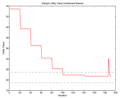
Figure 9: One sample objective function value of distributed Newton method against number of iterations. The dotted black lines denote $\pm 5\%$ interval of the optimal objective function value.

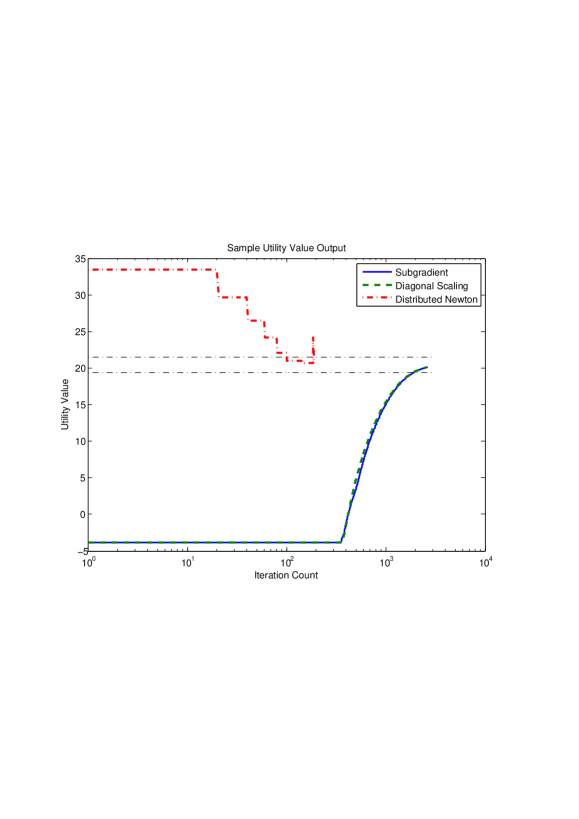
Figure 10: One sample objective function value of all three methods against log scaled iteration count. The dotted black lines denote $\pm 5\%$ interval of the optimal objective function value.

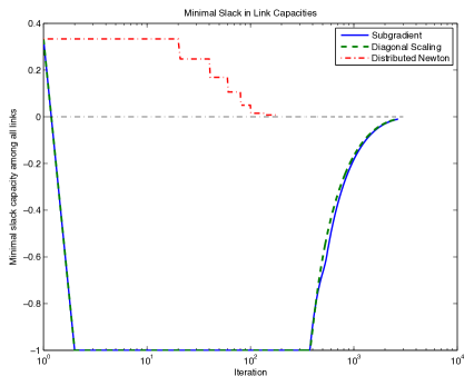
Figure 11: Sample minimal slack in link capacity of all three methods against log scaled iteration count. Negative slack means violating capacity constraint. The dotted black line denotes $0$.

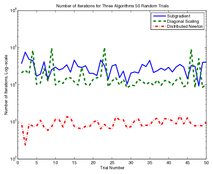
Figure 12: Log scaled iteration count for the 3 methods implemented over 50 randomly generated networks.

A sample evolution of the objective function value of the distributed Newton method is presented in Figure 9. This is generated for the network in Figure 1. The horizontal line segments correspond to the dual iterations, where the primal vector stays constant, and each jump in the figure is a primal Newton update. The spike close to the end is a result of rescaling and using a new barrier coefficient in the second round of the distributed Newton algorithm [cf. Section 5.3]. The black dotted lines indicate $\pm 5\%$ interval around the optimal objective function value.

The other two algorithms were implemented for the same problem, and the objective function values are plotted in Figure 10, with logarithmic scaled iteration count on the $x$-axis. We use black dotted lines to indicate $\pm 5\%$ interval around the optimal objective function value. While the subgradient and diagonal scaling methods have similar convergence behavior, the distributed Newton method significantly outperforms the two.

One of the important features of the distributed Newton method is that, unlike the other two algorithms, the generated primal iterates satisfy the link capacity constraint throughout the algorithm. This observation is confirmed by Figure 11, where the minimal slacks in links are shown for all three algorithms. The black dotted line is the zero line and a negative slack means violating the capacity constraint. The slacks that our distributed Newton method yields always stays above the zero line, while the other two only becomes feasible in the end.

To test the performances of the methods over general networks, we generated 50 random networks, with number of links $L=15$ and number of sources $S=8$. Each routing matrix consists of $L\times R$ Bernoulli random variables. All three methods are implemented over the 50 networks. We record the number of iterations upon termination for all 3 methods, and results are shown in Figure 12 on a log scale. The mean number of iterations to convergence from the 50 trials is $924$ for distributed Newton method, $20286$ for Newton-type diagonal scaling and $29315$ for subgradient method.

7 Conclusions

This paper develops a distributed Newton-type second order algorithm for network utility maximization problems, which can achieve superlinear convergence rate in primal iterates within some error neighborhood. We show that the computation of the dual Newton step can be implemented in a decentralized manner using a matrix splitting scheme. The key feature of this scheme is that its implementation uses an information exchange mechanism similar to that involved in first order methods applied to this problem. We show that even when the Newton direction and stepsize are computed with some error, the method achieves superlinear convergence rate in terms of primal iterations to an error neighborhood. Simulation results also indicate significant improvement over traditional distributed algorithms for network utility maximization problems. Possible future directions include a more detailed analysis of the relationship between the rate of convergence of the dual iterations and the underlying topology of the network and investigating convergence properties for a fixed finite truncation of dual iterations.

Appendix A Distributed Stepsize Computation

In this section, we describe a distributed procedure with finite termination to compute stepsize $d^{k}$ according to Eq. (42). We first note that in Eq. (42), the scalar $b\in(0,1)$ is predetermined and the only unknown term is the inexact Newton decrement $\tilde{\lambda}(x^{k})$. In order to compute the value of $\tilde{\lambda}(x^{k})$, we rewrite the inexact Newton decrement based on definition (39) as $\tilde{\lambda}(x^{k})=\sqrt{\sum_{i\in\mathcal{S}}(\Delta\tilde{x}_{i}^{k})^{2}(H_{k})_{ii}+\sum_{l\in\mathcal{L}}(\Delta\tilde{x}_{l+S}^{k})^{2}(H_{k})_{(l+S)(l+S)}}$, or equivalently,

$$\left(\tilde{\lambda}(x^{k})\right)^{2}=\sum_{i\in\mathcal{S}}(\Delta\tilde{x}_{i}^{k})^{2}(H_{k})_{ii}+\sum_{l\in\mathcal{L}}(\Delta\tilde{x}_{l+S}^{k})^{2}(H_{k})_{(l+S)(l+S)}.$$ (97)

In the sequel, we develop a distributed summation procedure to compute this quantity by aggregating the local information available on sources and links. A key feature of this procedure is that it respects the simple information exchange mechanism used by first order methods applied to the NUM problem: information about the links along the routes is aggregated and sent back to the sources using a feedback mechanism. Over-counting is avoided using a novel off-line construction, which forms an (undirected) auxiliary graph that contains information on sources sharing common links.

Given a network with source set $\mathcal{S}=\{1,2,\ldots,S\}$ (each associated with a predetermined route) and link set $\mathcal{L}=\{1,2,\ldots,L\}$, we define the set of nodes in the auxiliary graph as the set $\mathcal{S}$, i.e., each node corresponds to a source (or equivalently, a flow) in the original network. The edges are formed between sources that share common links according to the following iterative construction. In this construction, each source is equipped with a state (or color) and each link is equipped with a set (a subset of sources), which are updated using signals sent by the sources along their routes.

Auxiliary Graph Construction:

• Initialization: Each link $l$ is associated with a set $\Theta_{l}=\emptyset$. One arbitrarily chosen source is marked as grey, and the rest are marked as white. The grey source sends a signal $\{$label, $i\}$ to its route. Each link $l$ receiving the signal, i.e., $l\in L(i)$, adds $i$ to $\Theta_{l}$.

• Iteration: In each iteration, first the sources update their states and send out signals according to step (A). Each link $l$ then receives signals sent in step (A) from the sources $i\in S(l)$ and updates the set $\Theta_{l}$ according to step (B).

  • Each source $i$:

    • If it is white, it sums up $|\Theta_{l}|$ along its route, using the value $|\Theta_{l}|$ from the previous time.

      • If $\sum_{l\in L(i)}|\Theta_{l}|>0$, then the source $i$ is marked grey and it sends two signals $\{$neighbor, $i\}$ and $\{$label, $i\}$ to its route.

      • Else, i.e., $\sum_{l\in L(i)}|\Theta_{l}|=0$, source $i$ does nothing for this iteration.

    • Otherwise, i.e., it is grey, source $i$ does nothing.

  • Each link $l$:

    • If $\Theta_{l}=\emptyset$:

      • If it experiences signal $\{$label, $i\}$ passing through it, it adds $i$ to $\Theta_{l}$. When there are more than one such signals during the same iteration, only the smallest $i$ is added. The signal keeps traversing the rest of its route.

      • Otherwise link $l$ simply carries the signal(s) passing through it, if any, to the next link or node.

    • Else, i.e., $\Theta_{l}\neq\emptyset$:

      • If it experiences signal $\{$neighbor, $i\}$ passing through it, an edge $(i,j)$ with label $L_{l}$ is added to the auxiliary graph for all $j\in\Theta_{l}$, and then $i$ is added to the set $\Theta_{l}$. If there are more than one such signals during the same iteration, the sources are added sequentially, and the resulting nodes in the set $\Theta_{l}$ form a clique in the auxiliary graph. Link $l$ then stops the signal, i.e., it does not pass the signals to the next link or node.

      • Otherwise link $l$ simply carries the signal(s) passing through it, if any, to the next link or node.

• Termination: Terminate after $S-1$ number of iterations.

The auxiliary graph construction process for the sample network in Figure 13 is illustrated in Figure 14, where the left column reflects the color of the nodes in the original network and the elements of the set $\Theta_{l}$ (labeled on each link $l$), while the right column corresponds to the auxiliary graph constructed after each iteration.

We next investigate some properties of the auxiliary graph, which will be used in proving that our distributed summation procedure yields the corrects values.

Figure 13: A sample network with four sources and ten links. Each link shows the flows (or sources) using that link. This example will be used to illustrate different parts of the distributed stepsize computation in this section.

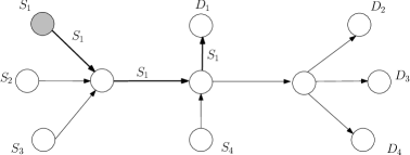
(a) State of the network $t=0$

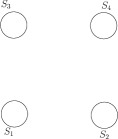
(b) State of the auxiliary graph $t=0$

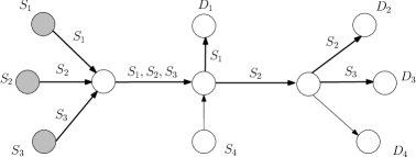
(c) State of the network $t=1$

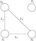
(d) State of the auxiliary graph $t=1$

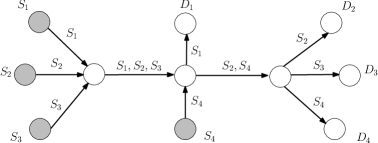
(e) State of the network $t=2$

(f) State of the auxiliary graph $t=2$

(g) State of the network $t=3$

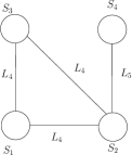
(h) State of the auxiliary graph $t=3$

Figure 14: Steps of the construction of the auxiliary graph corresponding to the network in Figure 13. The elements of $\Theta_{l}$ are labeled on link $l$. A link is drawn bold in the original graph if $\Theta_{l}\neq\emptyset$.

Lemma A.1.

Consider a network and its auxiliary graph with sets $\{\Theta_{l}\}_{l\in\mathcal{L}}$. The following statements hold:

• For each link $l$, $\Theta_{l}\subset S(l)$.

• Source nodes $i,j$ are connected in the auxiliary graph if and only if there exists a link $l$, such that $\{i,j\}\subset\Theta_{l}$.

• The auxiliary graph does not contain multiple edges, i.e., there exists at most one edge between any pair of nodes.

• The auxiliary graph is connected.

• For each link $l$, $\Theta_{l}\neq\emptyset$.

• There is no simple cycle in the auxiliary graph other than that formed by only the edges with the same label.

Proof.

We prove the above statements in the order they are stated.

• Part (1) follows immediately from our auxiliary graph construction, because each source only sends signals to links on its own route and the links only update their set $\Theta_{l}$ when they experience some signals passing through them.

• In the auxiliary graph construction, a link is added to the auxiliary graph only in step (B.b.1), where part (2) clearly holds.

• From the first two parts, there is an edge between source nodes $i,j$, i.e., $\{i,j\}\subset\Theta_{l}$ for some $l$, only if $i$ and $j$ share link $l$ in the original network. From the auxiliary graph construction, if sources $i$ and $j$ share link $l$ then an edge with label $L_{l}$ between $i$ and $j$ is formed at some iteration if and only if one of the following three cases holds:

  • In the beginning of the previous iteration $\Theta_{l}=\emptyset$ and sources $i,j$ are both white. During the previous iteration, source $i$ becomes grey and sends out the signal $\{$label,$i\}$ to link $l$, hence $\Theta_{l}=\{i\}$. In the current iteration, source $j$ with $\sum_{m\in L(j)}|\Theta_{m}|\geq|\Theta_{l}|>0$ becomes grey and sends out signal $\{$neighbor, $j\}$ to link $l$;

  • The symmetric case of I, where first source $j$ becomes grey and one iteration later source $i$ becomes grey.

  • In the beginning of the previous iteration $\Theta_{l}=\emptyset$ and sources $i,j$ are both white. During the previous iteration, some other source $t$ with $l\in L(t)$ becomes grey and sends out the signal $\{$label,$t\}$ to link $l$, hence $\Theta_{l}=\{t\}$. In the current iteration, both source $i$ and $j$ with $\sum_{m\in L(i)}|\Theta_{m}|\geq|\Theta_{l}|>0$ and $\sum_{m\in L(j)}|\Theta_{m}|\geq|\Theta_{l}|>0$ become grey and send out signals $\{$neighbor, $i\}$ and $\{$neighbor, $j\}$ to link $l$.

  Hence if an edge connecting nodes $i$ and $j$ exists in the auxiliary graph, then in the beginning of the iteration when the edge is formed at least one of the nodes is white, and by the end of the iteration both nodes are colored grey and stay grey. Therefore the edges between $i$ and $j$ in the auxiliary graph can only be formed during exactly one iteration.

  We next show that only one such edge can be formed in one iteration. The first two cases are symmetric, and without loss of generality we only consider cases I and III. In both of these cases, an edge between $i$ and $j$ is formed with label $L_{l}$ only if link $l$ receives the signal $\{$neighbor, $j\}$ and $\Theta_{l}\neq\emptyset$. In step (B.b.1) of the auxiliary graph construction, the first link with $\Theta_{l}\neq\emptyset$ stops the signal from passing to the rest of its route, hence at most one edge between $i$ and $j$ can be generated. Hence part (3) holds.

• By using a similar analysis as above, it is straightforward to see that if at one iteration source $i$ from the original network becomes grey, then in the next iteration all the sources which share link with $i$ become grey and are connected to $i$ in the auxiliary graph. By induction, we conclude that all the nodes in the auxiliary graph corresponding to sources colored grey in the original network are connected to the source node marked grey in the initialization step, and hence these nodes form a connected component.

  We next show that all nodes are colored grey when the auxiliary graph construction procedure terminates. We first argue that at least one node is marked grey from white at each iteration before all nodes are marked grey. Assume the contrary is true, that is at some iteration no more nodes are marked grey and there exists a set of white nodes $S^{*}$. This implies that the nodes in $S^{*}$ do not share any links with the nodes in $\mathcal{S}\backslash S^{*}$ and thus there is no path from any source in the set $\mathcal{S}\backslash S^{*}$ to any source in $S^{*}$ using the links (including the feedback mechanisms) in the original network. However, this contradicts the fact that all links form a strongly connected graph. Therefore after $S-1$ iterations all nodes in the original graph are colored grey and therefore we have the desired statement hold.

• Analysis for part (3) suggests that all the connected nodes in the auxiliary graph are colored grey. In view of the part (4), all the sources are colored grey when the auxiliary graph construction procedure terminates. Step (B.a.1) implies that a link has $\Theta_{l}=\emptyset$ if all sources $i\in S(l)$ are white. Since each link is used by at least one source, and all sources are grey, part (5) holds.

• We prove part (6) by showing the auxiliary graph, when the cycles formed by the edges of the same label are removed, is acyclic. For each link $l$, let $i_{l}^{*}$ denote the first element added to the set $\Theta_{l}$ in the auxiliary graph construction process, which is uniquely defined for each link $l$ by Step (B.a.1). In the set $\mathcal{S}$ for each link $l$, we define an equivalence class by $i\sim j$ if $\{i,j\}\subset\Theta_{l}\backslash\{i_{l}^{*}\}$, which implies if and only if $i$ and $j$ are connected in the auxiliary graph and $i\sim j$, this link is formed by scenario III as defined above in the proof of part (3).

  The nodes in each equivalence class are connected by edges with the same label, which form the undesired cycles. We remove these cycles by merging each equivalence class into one representative node, which inherits all the edges going between the nodes in the equivalence class and $\mathcal{S}\backslash\Theta_{l}$ in the auxiliary graph, and is connected to $i_{l}^{*}$ via one edge. Note the resulting graph is connected, since the auxiliary graph is by part (4) and all the remaining edges are generated under scenarios I and II as defined in the proof of part (3).

  We now show that the resulting graph contains no cycle. From cases I and II, it follows immediately that an edge is generated when one more source becomes grey. Therefore if number of noes is $N$, we have $N-1$ edges. In a connected graph, this implies we have a tree, i.e. acyclic, and hence part (6) holds.

∎

We denote the set of links inducing edges in the auxiliary graph as $L^{*}=\{l\mid|\Theta_{l}|>1\}$ and for each source $i$ the set of links which induce edges in the auxiliary graph as $L^{*}(i)=\{l\mid i\in\Theta_{l},l\in L^{*}\}$ for notational convenience. Each link can identify if it is in $L^{*}$ by the cardinality of the set $\Theta_{l}$. Each source $i$ can obtain $|L^{*}(i)|$ along the links on its route. The auxiliary graph remains the same throughout the distributed Newton algorithm and only depends on the structure of the network (independent of the utility functions and link capacities), therefore given a network, the above construction only needs to be preformed once prior to execution of the distributed Newton algorithm.

We next present a distributed procedure to compute the sum in Eq. (97) and show that the sets $\Theta_{l}$ constructed using the above procedure avoids over-counting and enables computation of the correct values.

Distributed Summation Procedure:

• Initialization: Each link $l$ initializes to $z_{l}(0)=0$. Each source $i$ computes $y_{i}^{*}=(\Delta\tilde{x}_{i}^{k})^{2}(H_{k})_{ii}$ and each link $l$ computes $z_{l}^{*}=\frac{1}{|S(l)|}(\Delta\tilde{x}_{l+S}^{k})^{2}(H_{k})_{(l+S)(l+S)}$. Each source $i$ aggregates the sum

  $$y_{i}(0)=y_{i}^{*}+\sum_{l\in L(i)}z_{l}^{*}$$ (98)

  along its route.

• Iteration for $t=1,2,\ldots,S$. The following 3 steps are completed in the order they are presented.

  • Each source $i$ sends its current value $y_{i}(t)$ to its route.

  • Each link $l$ uses the $y_{i}(t)$ received and computes

    $$z_{l}(t)=\sum_{i\in\Theta_{l}}y_{i}(t-1)-\left(|\Theta_{l}|-1\right)z_{l}(t-1).$$ (99)

  • Each source $i$ aggregates information along its route from the links $l\in L^{*}(i)$ and computes

    $$y_{i}(t)=\sum_{l\in L^{*}(i)}z_{l}(t)-\left(|L^{*}(i)|-1\right)y_{i}(t-1).$$ (100)

• Termination: Terminate after $S$ number of iterations.

(a) State of the network $t=0$

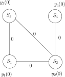
(b) State of auxiliary graph $t=0$

(c) State of the network $t=1$

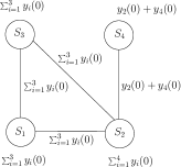
(d) State of auxiliary graph $t=1$

(e) State of the network $t=2$

(f) State of auxiliary graph $t=2$

(g) State of the network $t=3$

(h) State of auxiliary graph $t=3$

Figure 15: Evolution of distributed summation process, where $\rho_{i}=y_{i}(0)$ and destination node is indicated using a dot with the same color as its corresponding source.

(a) State of the network $t=4$

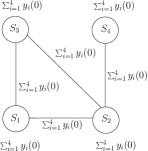
(b) State of auxiliary graph $t=4$

Figure 16: Evolution of distributed summation process continued, where $\rho_{i}=y_{i}(0)$ and destination node is indicated using a dot with the same color as its corresponding source.

By the diagonal structure of the Hessian matrix $H_{k}$, the scalars $(\Delta\tilde{x}_{i}^{k})^{2}(H_{k})_{ii}$ and $(\Delta\tilde{x}_{l+S}^{k})^{2}(H_{k})_{(l+S)(l+S)}$ are available to the corresponding source $i$ and link $l$ respectively, hence $z_{l}^{*}$ and $y_{i}^{*}$ can be computed using local information. In the above process, each source only uses aggregate information along its route and each link $l$ only uses information from sources $i\in S(l)$. The evolution of the distributed summation procedure for the sample network in Figure 13 is shown in Figures 15 and 16.

We next establish two lemmas, which quantifies the expansion of the $t$-hop neighborhood in the auxiliary graph for the links and sources. This will be key in showing that the aforementioned summation procedure yields the correct values at the sources and the links. For each source $i$, we use the notation $\mathcal{N}_{i}(t)$ to denote the set of nodes that are connected to node $i$ by a path of length at most $t$ in the auxiliary graph. Note that $\mathcal{N}_{i}(0)=\{i\}$. We say that node $i$ is $t$-hops away from node $j$ is the length of the shortest path between nodes $i$ and $j$ is $t$.

Lemma A.2.

Consider a network and its auxiliary graph with sets $\{\Theta_{l}\}_{l\in\mathcal{L}}$. For any link $l$ and all $t\geq 1$, we have,

$$\mathcal{N}_{i}(t)\cap\mathcal{N}_{j}(t)=\cup_{m\in\Theta_{l}}\mathcal{N}_{m}(t-1)\qquad\hbox{for }i,j\in\Theta_{l}\hbox{ with }i\neq j.$$ (101)

Proof.

Since the source nodes $i,j\in\Theta_{l}$, by part (2) of Lemma A.1, they are $1$-hop away from all other nodes in $\Theta_{l}$. Hence if a source node $n$ is in $\mathcal{N}_{m}(t-1)$ for $m\in\Theta_{l}$, then $n$ is at most $t$-hops away from $i$ or $j$. This yields

$$\cup_{m\in\Theta_{l}}\mathcal{N}_{m}(t-1)\subset\mathcal{N}_{i}(t)\cap\mathcal{N}_{j}(t).$$ (102)

On the other hand, if $n\in\mathcal{N}_{i}(t)\cap\mathcal{N}_{j}(t)$, then we have either $n\in\mathcal{N}_{i}(t-1)$ and hence $n\in\cup_{m\in\Theta_{l}}\mathcal{N}_{m}(t-1)$ or

$$n\in\left(\mathcal{N}_{i}(t)\backslash\mathcal{N}_{i}(t-1)\right)\cap\mathcal{N}_{j}(t).$$

Let $P(a,b)$ denote an ordered set of nodes on the path between nodes $a$ and $b$ including $b$ but not $a$ for notational convenience. Then the above relation implies there exists a path with $|P(i,n)|=t$ and $|P(j,n)|\leq t$. Let $n^{*}\in P(i,n)\cap P(j,n)$ and $P(j,n^{*})\cap P(j,n^{*})=\emptyset$. The node $n^{*}$ exists, because the two paths both end at $n$. If $n^{*}\not\in\Theta_{l}$, then we have a cycle of $\{P(i,n^{*}),P(n^{*},j),P(j,i)\}$, which includes an edge with label $L_{l}$ between $i$ and $j$ and other edges. In view of part (6) of Lemma A.1, this leads to a contradiction. Therefore we obtain $n^{*}\in\Theta_{l}$, implying $P(i,n)=\{P(i,n^{*}),P(n^{*},n)\}$. Since $i$ is connected to all nodes in $\Theta_{l}$, $|P(i,n^{*})|=1$ and hence $|P(n^{*},n)|=t-1$, which implies $n\in\mathcal{N}_{n^{*}}(t-1)\subset\cup_{m\in\Theta_{l}}\mathcal{N}_{m}(t-1)$. Therefore the above analysis yields

$$\mathcal{N}_{i}(t)\cap\mathcal{N}_{j}(t)\subset\cup_{m\in\Theta_{l}}\mathcal{N}_{m}(t-1).$$

With relation (102), this establishes the desired equality. ∎

Lemma A.3.

Consider a network and its auxiliary graph with sets $\{\Theta_{l}\}_{l\in\mathcal{L}}$. For any source $i$, and all $t\geq 1$, we have,

$$\left(\cup_{j\in\Theta_{l}}\mathcal{N}_{j}(t)\right)\cap\left(\cup_{j\in\Theta_{m}}\mathcal{N}_{j}(t)\right)=\mathcal{N}_{i}(t)\qquad\hbox{for }l,m\in L^{*}(i)\hbox{ with }l\neq m.$$ (103)

Proof.

Since $l,m\in L^{*}(i)$, we have $i\in\Theta_{l}$ and $i\in\Theta_{m}$, this yields,

$$\mathcal{N}_{i}(t)\subset\left(\cup_{j\in\Theta_{l}}\mathcal{N}_{j}(t)\right)\cap\left(\cup_{j\in\Theta_{m}}\mathcal{N}_{j}(t)\right).$$

On the other hand, assume there exists a node $n$ with $n\in\left(\cup_{j\in\Theta_{l}}\mathcal{N}_{j}(t)\right)\cap\left(\cup_{j\in\Theta_{m}}\mathcal{N}_{j}(t)\right)$, and $n\not\in\mathcal{N}_{i}(t)$. Then there exists a node $p\in\Theta_{l}$ with $p\neq i$ and $n\in\mathcal{N}_{p}(t)$. Similarly there exists a node $q\in\Theta_{m}$ with $q\neq i$ and $n\in\mathcal{N}_{q}(t)$. Let $P(a,b)$ denote an ordered set nodes on the path between nodes $a$ and $b$ including $b$ but not $a$ for notational convenience. Let $n^{*}\in P(p,n)\cap P(q,n)$ and $P(p,n^{*})\cap P(q,n^{*})=\emptyset$. The node $n^{*}$ exists, because the two paths both end at $n$. Since nodes $i,p$ are connected via an edge with label $L_{l}$ and $i,q$ are connected via an edge with label $L_{m}$, we have a cycle of $\{P(i,p),P(p,n),P(n,q),P(q,i)\}$, which contradicts part (6) in Lemma A.1 and we have

$$\left(\cup_{j\in\Theta_{l}}\mathcal{N}_{j}(t)\right)\cap\left(\cup_{j\in\Theta_{m}}\mathcal{N}_{j}(t)\right)\subset\mathcal{N}_{i}(t).$$

The preceding two relations establish the desired equivalence. ∎

Equipped with the preceding lemma, we can now show that upon termination of the summation procedure, each source $i$ and link $l$ have $y_{i}(S)=z_{l}(S-1)=(\tilde{\lambda}(x^{k}))^{2}$ [cf. Eq. (97)].

Theorem A.4.

Consider a network and its auxiliary graph with sets $\{\Theta_{l}\}_{l\in\mathcal{L}}$. Let $\Omega$ denote the set of all subsets of $S$ and define the function $\sigma:\Omega\to\mathbb{R}$ as

$$\sigma(K)=\sum_{l\in\cup_{i\in K}L(i)}z_{l}^{*}\sum_{i\in K}I_{\{l\in L(i)\}}+\sum_{i\in K}y_{i}^{*},$$

where $y_{i}^{*}=(\Delta\tilde{x}_{i}^{k})^{2}(H_{k})_{ii}$, $z_{l}^{*}=\frac{1}{|S(l)|}(\Delta\tilde{x}_{l+S}^{k})^{2}(H_{k})_{(l+S)(l+S)}$ and $I_{\{l\in L(i)\}}$ is the indicator function for the event $\{l\in L(i)\}$. Let $y_{i}(t)$ and $z_{l}(t)$ be the iterates generated by the distributed summation procedure described above. Then for all $t\in\{1,\ldots,S\}$, the value $z_{l}(t)$ at each link satisfies

$$z_{l}(t)=\sigma(\cup_{i\in\Theta_{l}}\mathcal{N}_{i}(t-1)),$$ (104)

and the value $y_{i}(t)$ at each source node satisfies

$$y_{i}(t)=\sigma(\mathcal{N}_{i}(t)).$$ (105)

Proof.

We use induction to prove the theorem.
Base case: $t=1$.
Since $z_{l}(0)=0$ for all links, Eq. (99) for $t=1$ is

$$z_{l}(1)=\sum_{i\in\Theta_{l}}y_{i}(0)=\sum_{i\in\Theta_{l}}(y_{i}^{*}+\sum_{l\in L(i)}z^{*}_{l})=\sigma(\Theta_{l}),$$

where we use the definition of $y(0)$ [cf. Eq. (98)] and the function $\sigma(\cdot)$. Since $\mathcal{N}_{i}(0)=i$, the above relation implies Eq. (104) holds.

For source $i$, from update relation (100), we have

$$y_{i}(1)=\sum_{l\in L^{*}(i)}\sigma(\Theta_{l})-\left(|L^{*}(i)|-1\right)y_{i}(0).$$

Lemma A.3 and inclusion-exclusion principle imply

$$\sum_{l\in L^{*}(i)}\sigma(\Theta_{l})=\sigma(\cup_{l\in L^{*}(i)}\Theta_{l})+\left(|L^{*}(i)|-1\right)\sigma(i).$$

Since $y_{i}(0)=\sigma(i)$ based on the definition of $y_{i}(0)$ [cf. Eq. (98)], by rearranging the preceding two relations, we obtain

$$y_{i}(1)=\sigma(\cup_{l\in L^{*}(i)}\Theta_{l})=\sigma(\mathcal{N}_{i}(1)),$$

which shows Eq. (105) holds for $t=1$.

Inductive step for $t=T\geq 2$.
Assume for $t=T-1$, Eqs. (105) and (104) hold, we first show that Eq. (104) hold. When $t=T$, by update equation (99), we obtain for link $l$

$$z_{l}(T)= \sum_{i\in\Theta_{l}}y_{i}(T-1)-\left(|\Theta_{l}|-1\right)z_{l}(T-1)$$

$$= \sum_{i\in\Theta_{l}}\sigma(\mathcal{N}_{i}(T-1))-\left(|\Theta_{l}|-1\right)z_{l}(T-1),$$

where the second equality follows from Eq. (105) for $t=T-1$.

If $|\Theta_{l}|=1$, then we have $z_{l}(T)=\sigma(\mathcal{N}_{i}(T-1))$, for $i\in\Theta_{l}$, therefore Eq. (104) is satisfied.

For $|\Theta_{l}|>1$, using Lemma A.2 for $t=T$ and by inclusion-exclusion principle, we obtain

$$\sum_{i\in\Theta_{l}}\sigma(\mathcal{N}_{i}(T-1))=\sigma\left(\cup_{i\in\Theta_{l}}\mathcal{N}_{i}(T-1)\right)+\left(|\Theta_{l}|-1\right)\sigma(\cup_{m\in\Theta_{l}}\mathcal{N}_{m}(T-2)).$$

Eq. (104) for $t=T-1$ yields $z_{l}(T-1)=\sigma(\cup_{m\in\Theta_{l}}\mathcal{N}_{m}(T-2))$. By using this fact and rearranging the preceding two relations, we have Eq. (104) holds for $t=T$, i.e.,

$$z_{l}(T)=\sigma\left(\cup_{i\in\Theta_{l}}\mathcal{N}_{i}(T-1)\right).$$

We next establish Eq. (105). From update equation (100), using the preceding relation, we have

$$y_{i}(T)= \sum_{l\in L^{*}(i)}z_{l}(T)-\left(|L^{*}(i)|-1\right)y_{i}(T-1)$$

$$= \sum_{l\in L^{*}(i)}\sigma\left(\cup_{i\in\Theta_{l}}\mathcal{N}_{i}(T-1)\right)-\left(|L^{*}(i)|-1\right)y_{i}(T-1).$$

Lemma A.3 and inclusion-exclusion principle imply

$$\sum_{l\in L^{*}(i)}\sigma\left(\cup_{i\in\Theta_{l}}\mathcal{N}_{i}(T-1)\right)=\sigma(\cup_{l\in L^{*}(i)}\cup_{i\in\Theta_{l}}\mathcal{N}_{i}(T-1))+\left(|L^{*}(i)|-1\right)\sigma(\mathcal{N}_{i}(T-1)).$$

By definition of $\mathcal{N}_{i}(\cdot)$, we have $\cup_{l\in L^{*}(i)}\cup_{i\in\Theta_{l}}\mathcal{N}_{i}(T-1)=\mathcal{N}_{i}(T)$. By using Eq. (105) for $t=T-1$, i.e., $y_{i}(T-1)=\sigma(\mathcal{N}_{i}(T-1))$ and rearranging the above two equations, we obtain

$$y(T)=\sigma(\mathcal{N}_{i}(T)),$$

which completes the inductive step.∎

Using definition of the function $\sigma(\cdot)$, we have $(\tilde{\lambda}(x^{k}))^{2}=\sigma(\mathcal{S})$. By the above theorem, we conclude that after $S$ iterations,

$$y_{i}(S)=\sigma(\mathcal{N}_{i}(S))=\sigma(\mathcal{S})=(\tilde{\lambda}(x^{k}))^{2}.$$

By observing that $\cup_{i\in\Theta_{l}}\mathcal{N}_{i}(S-1)=\mathcal{S}$, we also have

$$z_{i}(S-1)=\sigma\left(\cup_{i\in\Theta_{l}}\mathcal{N}_{i}(S-1)\right)=\sigma(\mathcal{S}))=(\tilde{\lambda}(x^{k}))^{2},$$

where we used part (5) of Lemma A.1. This shows that the value $\tilde{\lambda}(x^{k})^{2}$ is available to all sources and links after $S-1$ iterations.

Note that the number $S$ is an upper bound on the number of iterations required in the distributed summation process to obtain the correct value at the links and sources in the original graph. If the value of the diameter of the auxiliary graph (or an upper bound on it) is known, then the process would terminate in number of steps equal to this value plus 1. For instance, when all the sources share one common link, then the auxiliary graph is a complete graph, and only $2$ iterations is required. On the other hand, when the auxiliary graph is a line, the summation procedure would take $S$ iterations.

We finally contrast our distributed summation procedure with spanning tree computations, which were used widely in 1970s and 1980s for performing information exchange among different processors in network flow problems. In spanning tree based approaches, information from all processors is passed along the edges of a spanning tree, and stored at and broadcast by a designated central root node (see [23] and [10]). In contrast, our summation procedure involves (scalar) information aggregated along the routes and fed back independently to different sources, which is a more natural exchange mechanism in an environment with decentralized sources. Moreover, processors in the system (i.e., sources and links) do not need to maintain predecessor/successor information (as required by spanning tree methods). The only network-related information is the sets $\theta_{l}$ for $l\in\mathcal{L}$ kept at the individual links and obtained from the auxiliary graph, which is itself constructed using the feedback mechanism described above.

Appendix B Distributed Error Checking

In this section, we present a distributed error checking method to determine when to terminate the dual computation procedure to meet the error tolerance level in Assumption 2 at a primal iteration $k$. The method involves two stages: in the first stage, the links and sources execute a predetermined number of dual iterations. In the second stage, if the error tolerance level is not satisfied in the previous stage, the links and sources implement dual iterations until some distributed termination criteria is met. For the rest of this section we suppress the dependence of the dual vector on the primal iteration index $k$ for notational convenience and we adopt the following assumption on the information available to each node and link.

Assumption 5.

There exists a positive scalar $F<1$ such that the spectral radius of the matrix $M=(D_{k}+\bar{B}_{k})^{-1}(\bar{B}_{k}-B_{k})$ satisfies $\rho(M)\leq F$. Each source and link knows the scalar $F$ and the total number of sources and links in the graph, denoted by $S$ and $L$ respectively.

As noted in Section 4.2, the matrix $M=(D_{k}+\bar{B}_{k})^{-1}(\bar{B}_{k}-B_{k})$ is the weighted Laplacian matrix of the dual graph, therefore the bound $F$ can be obtained once the structure of the dual graph is known [12], [7]. In this assumption, we only require availability of some aggregate information, and hence the distributed nature of the algorithm is preserved. Before we introduce the details of the algorithm, we establish a relation between $\left|\left|w^{*}-w(t)\right|\right|_{\infty}$ and $\left|\left|w(t+1)-w(t)\right|\right|_{\infty}$, which is a key relation in developing the distributed error checking method.

Lemma B.1.

Let the matrix $M$ be $M=(D_{k}+\bar{B}_{k})^{-1}(\bar{B}_{k}-B_{k})$. Let $w(t)$ denote the dual variable generated by iteration (26), and $w^{*}$ be the fixed point of the iteration. Let $F$ and $L$ be the positive scalar defined in Assumption 5. Then the following relation holds,

$$\left|\left|w^{*}-w(t)\right|\right|_{\infty}\leq\frac{\sqrt{L}}{1-F}\left|\left|w(t+1)-w(t)\right|\right|_{\infty}.$$ (106)

Proof.

Iteration (26) implies that the fixed point $w^{*}$ satisfies the following relation,

$$w^{*}=Mw^{*}+(D_{k}+\bar{B}_{k})^{-1}(-AH_{k}^{-1}\nabla f(x^{k})),$$

and the iterates $w(t)$ satisfy,

$$w(t+1)=Mw(t)+(D_{k}+\bar{B}_{k})^{-1}(-AH_{k}^{-1}\nabla f(x^{k})).$$

By combining the above two relations, we obtain,

$$w(t+1)-w(t)=(I-M)(w^{*}-w(t)).$$

Hence, by the definition of matrix infinity norm, we have

$$\left|\left|w^{*}-w(t)\right|\right|_{\infty}\leq\left|\left|(1-M)^{-1}\right|\right|_{\infty}\left|\left|w(t+1)-w(t)\right|\right|_{\infty}.$$

Using norm equivalence for finite dimensional Euclidean space and theories of linear algebra, we obtain $\left|\left|(I-M)^{-1}\right|\right|_{\infty}\leq\sqrt{L}\left|\left|(I-M)^{-1}\right|\right|_{2}\leq\frac{\sqrt{L}}{1-\left|\left|M\right|\right|_{2}}$ [16], [2]. For the symmetric real matrix $M$ we have $\rho(M)=\left|\left|M\right|\right|_{2}$, and hence we obtain the desired relation. ∎

We next use the above lemma to develop two theorems each of which serves as a starting point for one of the stages of the distributed error checking method.

Theorem B.2.

Let $\{x^{k}\}$ be the primal sequence generated by the inexact Newton method (37) and $H_{k}$ be the corresponding Hessian matrix at the $k^{th}$ iteration. Let $w(t)$ be the inexact dual variable obtained after $t$ dual iterations (26) and $w^{*}$ be the exact solution to (17), i.e. the limit of the sequence $\{w(t)\}$ as $t\to\infty$. Let vectors $\Delta x^{k}$ and $\Delta\tilde{x}^{k}$ be the exact and inexact Newton directions obtained using $w^{*}$ and $w(t)$ [cf. Eqs. (35)-(36)], and vector $\gamma^{k}$ be the error in the Newton direction computation at $x^{k}$ , defined by $\gamma^{k}=\Delta x^{k}-\Delta\tilde{x}^{k}$. For some positive scalar $p$, let

$$\rho_{i}=\left|\frac{\sqrt{L}(H_{k}^{-1})_{ii}|L(i)|\left|\left|w(t+1)-w(t)\right|\right|_{\infty}}{(1-F)(H_{k}^{-1})_{ii}[R^{\prime}]^{i}w(t)}\right|$$ (107)

for each source $i$, and

$$\rho_{l}=\left|\frac{\sqrt{L}\sum_{i\in S(l)}(H_{k}^{-1})_{ii}|L(i)|\left|\left|w(t+1)-w(t)\right|\right|_{\infty}}{(1-F)\sum_{i\in S(l)}(H_{k}^{-1})_{ii}[R^{\prime}]^{i}w(t)}\right|$$ (108)

for each link $l$. Define a nonnegative scalar $\beta^{k}$ as

$$\beta^{k}=\left(\max\left\{\max_{i\in\mathcal{S}}\frac{\rho_{i}}{p},\max_{l\in\mathcal{L}}\frac{\rho_{l}}{p}\right\}\right)^{-2}.$$ (109)

Then we have

$$\beta^{k}(\gamma^{k})^{\prime}H_{k}\gamma^{k}\leq p^{2}(\Delta\tilde{x}^{k})^{\prime}H_{k}(\Delta\tilde{x}^{k}).$$ (110)

Proof.

For notational convenience, we let matrix $P_{k}$ denote the $S\times S$ principal submatrix of $H_{k}$, i.e. $(P_{k})_{ii}=(H_{k})_{ii}$ for $i\leq S$, vector $\Delta\tilde{s}$ in $\mathbb{R}^{S}$ denote the first $S$ components of the vector $\Delta\tilde{x}^{k}$, vector $\Delta\tilde{y}_{l}$ in $\mathbb{R}^{L}$ denote the last $L$ components of the vector $\Delta\tilde{x}^{k}$. Similarly, we denote by $\Delta s$ and $\Delta y$ the first $S$ and last $L$ components of the exact Newton direction $\Delta x$ respectively. From Eq. (35), we have for each $i\in S$,

$$\left|\frac{\Delta s_{i}-\Delta\tilde{s}_{i}}{\Delta\tilde{s}_{i}}\right| =\left|\frac{(H_{k}^{-1})_{ii}[R^{\prime}]^{i}(w^{*}-w(t))}{(H_{k}^{-1})_{ii}[R^{\prime}]^{i}w(t)}\right|$$

$$\leq\left|\frac{(H_{k}^{-1})_{ii}[R^{\prime}]^{i}e\left|\left|w^{*}-w(t)\right|\right|_{\infty}}{(H_{k}^{-1})_{ii}[R^{\prime}]^{i}w(t)}\right|$$

$$\leq\left|\frac{\sqrt{L}(H_{k}^{-1})_{ii}|L(i)|\left|\left|w(t+1)-w(t)\right|\right|_{\infty}}{(1-F)(H_{k}^{-1})_{ii}[R^{\prime}]^{i}w(t)}\right|=\rho_{i},$$

where the first inequality follows from the element-wise nonnegativity of matrices $H_{k}$ and $R$, and the second inequality follows from relation (106).

Similarly for each link $l\in L$, by relations (35) and (36) we obtain

$$\left|\frac{\Delta y_{l}-\Delta\tilde{y}_{l}}{\Delta\tilde{y}_{l}}\right| =\left|\frac{[R]^{l}P_{k}^{-1}R^{\prime}(w^{*}-w(t))}{[R]^{l}P_{k}^{-1}R^{\prime}w(t)}\right|$$

$$\leq\left|\frac{\sum_{i\in S(l)}(P_{k}^{-1})_{ii}R^{\prime}e\left|\left|w^{*}-w(t)\right|\right|_{\infty}}{\sum_{i\in S(l)}(P_{k}^{-1})_{ii}[R^{\prime}]^{i}w(t)}\right|$$

$$\leq\left|\frac{\sqrt{L}\sum_{i\in S(l)}(H_{k}^{-1})_{ii}|L(i)|\left|\left|w(t+1)-w(t)\right|\right|_{\infty}}{(1-F)\sum_{i\in S(l)}(H_{k}^{-1})_{ii}[R^{\prime}]^{i}w(t)}\right|=\rho_{l},$$

where the first inequality follows from the structure of the matrix $R$ and the element-wise nonnegativity of matrices $H_{k}$ and $R$, and the second inequality follows from relation (106) and the definition for matrix $P_{k}$.

The definition for $\beta^{k}$ [cf. Eq. (109)] implies that

$$\frac{p}{\sqrt{\beta^{k}}}=\max\left\{\max_{i\in\mathcal{S}}\rho_{i},\max_{l\in\mathcal{L}}\rho_{l}\right\}.$$

Therefore the preceding relations imply that $\left|\frac{\Delta s_{i}-\Delta\tilde{s}_{i}}{\Delta\tilde{s}_{i}}\right|\leq\frac{p}{\sqrt{\beta^{k}}}$ and $\left|\frac{\Delta y_{l}-\Delta\tilde{y}_{l}}{\Delta\tilde{y}_{l}}\right|\leq\frac{p}{\sqrt{\beta^{k}}}$, i.e.,

$$\sqrt{\beta^{k}}\left|\gamma^{k}_{i}\right|\leq p|{\Delta\tilde{x}_{i}}|,$$

which implies the desired relation.

∎

Theorem B.3.

Let $\{x^{k}\}$ be the primal sequence generated by the inexact Newton method (37) and $H_{k}$ be the corresponding Hessian matrix at $k^{th}$ iteration. Let $w(t)$ be the inexact dual variable obtained after $t$ dual iterations (26) and $w^{*}$ be the exact solution to (17), i.e. the limit of the sequence $\{w(t)\}$ as $t\to\infty$. Let vectors $\Delta x^{k}$ and $\Delta\tilde{x}^{k}$ be the exact and inexact Newton directions obtained using $w^{*}$ and $w(t)$ [cf. Eqs. (35)-(36)] respectively, and vector $\gamma^{k}$ be the error in the Newton direction computation at $x^{k}$ , defined by $\gamma^{k}=\Delta x^{k}-\Delta\tilde{x}^{k}$. For some scalar $\beta$ and $\epsilon$ where $0<\beta^{k}<1$ and $\epsilon>0$, let

$$h_{i}=\sqrt{\frac{\epsilon}{(1-\beta^{k})(L+S)L}}\frac{1-F}{|L(i)|(H_{k}^{-\frac{1}{2}})_{ii}}$$ (111)

for each source $i$, and

$$h_{l}=\sqrt{\frac{\epsilon}{(1-\beta^{k})(L+S)L}}\frac{1-F}{(H_{k}^{\frac{1}{2}})_{(S+l)(S+l)}\sum_{i\in S(L)}|L(i)|(H_{k})_{ii}^{-1}}$$ (112)

for each link $l$. Define a nonnegative scalar $h$ as

$$h=\left(\min\left\{\min_{i\in\mathcal{S}}h_{i},\min_{l\in\mathcal{L}}h_{l}\right\}\right).$$ (113)

Then the condition

$$\left|\left|w(t+1)-w(t)\right|\right|_{\infty}\leq h$$ (114)

implies

$$(\gamma^{k})^{\prime}H_{k}\gamma^{k}\leq\frac{\epsilon}{1-\beta^{k}}.$$ (115)

Proof.

We let matrix $P_{k}$ denote the $S\times S$ principal submatrix of $H_{k}$, i.e. $(P_{k})_{ii}=(H_{k})_{ii}$ for $i\leq S$, for notational convenience. The definition of $h$ [cf. Eq. (113)] and relation (114) implies

$$\left|\left|w(t+1)-w(t)\right|\right|_{\infty}\leq h_{i},\in\mathcal{S},$$

and

$$\left|\left|w(t+1)-w(t)\right|\right|_{\infty}\leq h_{l},\mbox{\quad for l }\in\mathcal{L},$$

Using relation (106) and the definition of $h_{i}$ and $h_{l}$ [cf. Eqs. (111) and (112)], the above two relations implies respectively that

$$\left|\left|w^{*}-w(t)\right|\right|_{\infty}\leq\sqrt{\frac{\epsilon}{(1-\beta^{k})(L+S)}}\frac{1}{|L(i)|(H_{k}^{-\frac{1}{2}})_{ii}},\mbox{\quad for i }\in\mathcal{S},$$ (116)

and

$$\left|\left|w^{*}-w(t)\right|\right|_{\infty}\leq\sqrt{\frac{\epsilon}{(1-\beta^{k})(L+S)}}\frac{1}{(H_{k}^{\frac{1}{2}})_{(S+l)(S+l)}\sum_{i\in S(L)}|L(i)|(H_{k})_{ii}^{-1}},\mbox{\quad for l }\in\mathcal{L}.$$ (117)

By using the element-wise nonnegativity of matrices $H$ and $A$, we have for each source $i$,

$$\left|(H_{k}^{-\frac{1}{2}})_{ii}[R^{\prime}]^{i}(w^{*}-w(t))\right|\leq(H_{k}^{-\frac{1}{2}})_{ii}[R^{\prime}]^{i}e\left|\left|w^{*}-w(t)\right|\right|_{\infty}=|L(i)|(H_{k}^{-\frac{1}{2}})_{ii}\left|\left|w^{*}-w(t)\right|\right|_{\infty},$$

where the last equality follows from the fact that $[R^{\prime}]^{i}e=|L(i)|$ for each source $i$.

The above inequality and relation (116) imply

$$\left|(H_{k}^{-\frac{1}{2}})_{ii}[R^{\prime}]^{i}(w^{*}-w(t))\right|\leq\sqrt{\frac{\epsilon}{(1-\beta^{k})(L+S)}}.$$ (118)

By the definition of matrices $P_{k}$ and $R$, we have for each link $l$,

$$\left|\right.(H_{k}^{\frac{1}{2}})_{(S+l)(S+l)}\left(\right.RP_{k}^{-1}R^{\prime}(w^{*}- w(t))\left.\right)^{l}\left.\right|\leq(H_{k}^{\frac{1}{2}})_{(S+l)(S+l)}[R]^{l}P_{k}^{-1}R^{\prime}e\left|\left|w^{*}-w(t)\right|\right|_{\infty}$$

$$=(H_{k}^{\frac{1}{2}})_{(S+l)(S+l)}\sum_{i\in S(l)}|L(i)|(H_{k}^{-1})_{ii}\left|\left|w^{*}-w(t)\right|\right|_{\infty}.$$

When combined with relation (117), the preceding relation yields

$$\left|(H_{k}^{\frac{1}{2}})_{(S+l)(S+l)}\left(RP_{k}^{-1}R^{\prime}(w^{*}-w(t))\right)^{l}\right|\leq\sqrt{\frac{\epsilon}{(1-\beta^{k})(L+S)}}.$$ (119)

From Eqs. (35)-(36) and the definition of $\gamma$, we have

$$\gamma^{k}_{i}=-\left(\begin{array}[]{c}P_{k}^{-1}R^{\prime}(w^{*}-w(t))\\ RP_{k}^{-1}R^{\prime}(w^{*}-w(t))\end{array}\right),$$

which implies that

$$(\gamma^{k})^{\prime}H_{k}\gamma^{k} =\sum_{i\in\mathcal{S}}\left((H_{k}^{-\frac{1}{2}})_{ii}[R^{\prime}]^{i}(w^{*}-w(t))\right)^{2}+\sum_{l\in\mathcal{L}}\left((H_{k}^{\frac{1}{2}})_{(S+l)(S+l)}\left(RP_{k}^{-1}R^{\prime}(w^{*}-w(t))\right)^{l}\right)^{2}$$

$$\leq\frac{\epsilon}{1-\beta^{k}},$$

where the inequality follows from (118), (119), which establishes the desired relation.

∎

We develop the distributed error checking method based on the preceding two theorems:

• Stage 1: The links and sources implement $T$ iterations of (26), where $T$ is a predetermined globally known constant. The links and sources then use Theorem B.2 with $t=T-1$ and $p$ as the desired relative error tolerance level defined in Assumption 2 to obtain a value $\beta^{k}$. If $\beta^{k}\geq 1$, then the dual iteration terminates.

• Stage 2: The links and sources use Theorem B.3 with $\beta^{k}$ obtained in the first stage and $\epsilon$ defined in Assumption 2 to obtain value $h$. Then they perform more iterations of the form (26) until the criterion (114) is satisfied.

Stage 1 corresponds to checking the term $p^{2}(\Delta\tilde{x}^{k})^{\prime}H_{k}(\Delta\tilde{x}^{k})$, while Stage 2 corresponds to the term $\epsilon$ in the error tolerance level. If the method terminates the dual iterations in Stage 1, then Assumption 2 is satisfied for any $\epsilon>0$; otherwise, by combining relations (110) and (115), we have

$$(\gamma^{k})^{\prime}H_{k}\gamma^{k}=(\beta^{k}+(1-\beta^{k}))(\gamma^{k})^{\prime}H_{k}\gamma^{k}\leq p^{2}(\Delta\tilde{x}^{k})^{\prime}H_{k}(\Delta\tilde{x}^{k})+\epsilon,$$

which shows that the error tolerance level in Assumption 2 is satisfied.

To show that the above method can be implemented in a distributed way, we first rewrite the terms $\rho_{i}$, $\rho_{l}$, $h_{i}$ and $h_{l}$ and analyze the information required to compute them in a decentralized way. We use the definition of the weighted price of the route $\Pi_{i}(t)$ and obtain $\Pi_{i}(t)=(H_{k}^{-1})_{ii}\sum_{l\in L(i)}w(t)=(H_{k}^{-1})_{ii}[R^{\prime}]^{i}w(t)$ and $\Pi_{i}(0)=(H_{k}^{-1})_{ii}|L(i)|$, where $w_{l}(0)=1$ for all links $l$. Therefore relations (107) and (108) can be rewritten as

$$\rho_{i}=\left|\frac{\sqrt{L}\Pi_{i}(0)\left|\left|w(t+1)-w(t)\right|\right|_{\infty}}{(1-F)\Pi_{i}(t)}\right|,$$

$$\rho_{l}=\left|\frac{\sqrt{L}\sum_{i\in S(l)}\Pi_{i}(0)\left|\left|w(t+1)-w(t)\right|\right|_{\infty}}{(1-F)\sum_{i\in S(l)}\Pi_{i}(t)}\right|.$$

Similarly, relations (111) and (112) can be transformed into

$$h_{i}=\sqrt{\frac{\epsilon}{(1-\beta^{k})(L+S)L}}\frac{1-F}{\pi_{i}(0)(H_{k}^{-\frac{1}{2}})_{ii}},$$

$$h_{l}=\sqrt{\frac{\epsilon}{(1-\beta^{k})(L+S)L}}\frac{1-F}{(H_{k}^{\frac{1}{2}})_{(S+l)(S+l)}\sum_{i\in S(L)}\Pi_{i}(0)}.$$

In our dual variable computation procedure, the values $\pi_{i}(0)$, $\Pi_{i}(0)$ and $\Pi_{i}(t)$ are made available to all the links source $i$ traverses through the feedback mechanism described in Section 4.2. Each source and node knows its local Hessian, i.e., $(H_{k})_{ii}$ for source $i$ and $(H_{k})_{(S+l)(S+l)}$ for link $l$. The value $\beta^{k}$ is available from the previous stage. Therefore in the above four expressions, the only not immediately available information is $\left|\left|w(t+1)-w(t)\right|\right|_{\infty}$, which can be obtained using a maximum consensus algorithm. Based on these four terms, the values of $\beta^{k}$ and $h$ can be obtained using once again maximum consensus and hence all the components necessary for the error checking method can be computed in a distributed way.

We observe that in the first $T$ iterations, i.e., Stage 1, only two executions of maximum consensus algorithms is required, where one is used to compute $\left|\left|w(t+1)-w(t)\right|\right|_{\infty}$ and the other for $\beta^{k}$. On the other hand, even though the computation of the value $h$ in Stage 2 needs only one execution of the maximum consensus algorithm, the term $\left|\left|w(t+1)-w(t)\right|\right|_{\infty}$ needs to be computed at each dual iteration $t$. Therefore the error checking in Stage 1 can be completed much more efficiently than in Stage 2. Hence, when we design values $p$ and $\epsilon$ in Assumption 2, we should choose $p$ to be relatively large, which results in an error checking method that does not enter Stage 2 frequently, and is hence faster.

References

• [1] S. Athuraliya and S. Low. Optimization flow control with Newton-like algorithm. Journal of Telecommunication Systems, 15:345–358, 2000.
• [2] A. Berman and R. J. Plemmons. Nonnegative Matrices in the Mathematical Sciences. Academic Press, New York, 1979.
• [3] D. P. Bertsekas. Convex Optimization Theory. Athena Scientific, 2009.
• [4] D. P. Bertsekas and E. M. Gafni. Projected Newton Methods and Optimization of Multicommodity Flows. IEEE Transactions on Automatic Control, 28(12), 1983.
• [5] D. P. Bertsekas, A. Nedic, and A. E. Ozdaglar. Convex Analysis and Optimization. Athena Scientific, Cambridge, MA, 2003.
• [6] D. Bickson, Y. Tock, A. Zymnis, S. Boyd, and D. Dolev. Distributed large scale network utility maximization. Proceedings of the 2009 IEEE International Conference on Symposium on Information Theory, 2, 2009.
• [7] N. Biggs. Algebraic Graph Theory. Cambridge University Press, second edition, 1993.
• [8] V. D. Blondel, J. M. Hendrickx, A. Olshevsky, and J. N. Tsitsiklis. Convergence in multiagent coordination, consensus, and flocking. Proceedings of IEEE CDC, 2005.
• [9] S. Boyd and L. Vandenberghe. Convex Optimization. Cambridge University Press, 2004.
• [10] G. H. Bradley, G. G. Brown, and G. W. Graves. Design and implementation of large scale primal transshipment algorithms. Management Science, 24(1):1–34, 1977.
• [11] M. Chiang, S. H. Low, A. R. Calderbank, and J.C. Doyle. Layering as optimization decomposition: a mathematical theory of network architectures. Proceedings of the IEEE, 95(1):255–312, 2007.
• [12] F. R. K. Chung. Spectral Graph Theory (CBMS Regional Conference Series in Mathematics). No. 92, American Mathematical Society, 1997.
• [13] R. Cottle, J. Pang, and R. Stone. The Linear Complementarity Problem. Academic Press, 1992.
• [14] R. Dembo, S. Eisenstat, and T. Steihaug. Inexact Newton Methods. SIAM Journal on Numerical Analysis, 19, 1982.
• [15] A. V. Fiacco and G. P. McCormick. Nonlinear Programming: Sequential Unconstrained Minimization Techniques. SIAM, 1990.
• [16] R. Horn and C. R. Johnson. Matrix Analysis. Cambridge University Press, New York, 1985.
• [17] A. Jadbabaie, J. Lin, and S. Morse. Coordination of groups of mobile autonomous agents using nearest neighbor rules. IEEE Transactions on Automatic Control, 48(6):988–1001, 2003.
• [18] A. Jadbabaie, A. Ozdaglar, and M. Zargham. A Distributed Newton method for network optimization. Proc. of CDC, 2009.
• [19] F. Jarre. Interior-point methods for convex programming. Applied Mathematics and Optimization, 26:287–311, 1992.
• [20] C. T. Kelley. Iterative Methods for Linear and Nonlinear Equations. SIAM, Philadelphia, PA, 1995.
• [21] F. Kelly. Charging and rate control for elastic traffic. European Transactions on Telecommunications, 8:33–37, 1997.
• [22] F. P. Kelly, A. K. Maulloo, and D. K. Tan. Rate control for communication networks: shadow prices, proportional fairness, and stability. Journal of the Operational Research Society, 49:237–252, 1998.
• [23] J. G. Klincewicz. A Newton Method for Convex Separable Network Flow Problems. Networks, 13:427–442, 1983.
• [24] D. C. Lay. Linear Algebra and Its Applications. Person Education, third edition, 2006.
• [25] S. H. Low and D. E. Lapsley. Optimization flow control, I: basic algorithm and convergence. IEEE/ACM Transaction on Networking, 7(6):861–874, 1999.
• [26] B. Mohar. Some Applications of Laplace Eigenvalues of Graphs. In: Hahn, G. and Sabidussi, G. (Eds.) Graph Symmetry: Algebraic Methods and Applications, NATO ASI Series C 497:227–275, 1997.
• [27] A. Nedic and A. Ozdaglar. Convex Optimization in Signal Processing and Communications, chapter Cooperative distributed multi-agent optimization. Eds., Eldar, Y. and Palomar, D., Cambridge University Press, 2008.
• [28] A. Nedic and A. Ozdaglar. Distributed subgradient methods for multi-agent optimization. Automatic Control, IEEE Transactions on, 54(1):48 –61, Jan 2009.
• [29] A. Nedic and A. Ozdaglar. Convergence rate for consensus with delays. Journal of Global Optimization, 47(3):437–456, 2010.
• [30] Y. Nesterov and A. Nemirovskii. Interior-Point Polynomial Algorithms in Convex Programming. SIAM, 2001.
• [31] R. Olfati-Saber and R. M. Murray. Consensus problems in networks of agents with switching topology and time-delays. IEEE Transactions on Automatic Control, 49(9):1520–1533, 2004.
• [32] A. Olshevsky and J. Tsitsiklis. Convergence speed in distributed consensus and averaging. SIAM Journal on Control and Optimization, 48(1):33–35, 2009.
• [33] R. Srikant. The Mathematics of Internet Congestion Control (Systems and Control: Foundations and Applications). Birkhäuser Boston, 2004.
• [34] J. N. Tsitsiklis. Problems in Decentralized Decision Making and Computation. PhD thesis, Dept. of Electrical Engineering and Computer Science, Massachusetts Institute of Technology, 1984.
• [35] J. N. Tsitsiklis, D. P. Bertsekas, and M. Athans. Distributed asynchronous deterministic and stochastic gradient optimization algorithms. IEEE Transactions on Automatic Control, 31(9):803–812, 1986.
• [36] R. Varga. Matrix Iterative Analysis. Prentice-Hall, Inc, Englewood Cliffs, NJ, 1965.
• [37] R. Varga. Gershgorin and His Circles. Springer Series in Computational Mathematics, 2004.