Reconstructing particle masses from pairs of decay chains

Abstract:

A method is proposed for determining the masses of the new particles $N,X,Y,Z$ in collider events containing a pair of effectively identical decay chains $Z\to Y+$ jet, $Y\to X+l_{1}$, $X\to N+l_{2}$, where $l_{1},l_{2}$ are opposite-sign same-flavour charged leptons and $N$ is invisible. By first determining the upper edge of the dilepton invariant mass spectrum, we reduce the problem to a curve for each event in the 3-dimensional space of mass-squared differences. The region through which most curves pass then determines the unknown masses. A statistical approach is applied to take account of mismeasurement of jet and missing momenta. The method is easily visualized and rather robust against combinatorial ambiguities and finite detector resolution. It can be successful even for small event samples, since it makes full use of the kinematical information from every event.

1 Introduction

One of the principal objectives of the ongoing experiments at the Large Hadron Collider is the discovery of new physics beyond the Standard Model. Many models of BSM physics predict a rich spectrum of new particles with sequential decays into chains of other new particles plus visible jets and leptons. Typically the endpoint of the chain is a new stable invisible particle that is a dark matter candidate. Important examples are the squark decay chain in supersymmetric models,

$$\tilde{q}\to\tilde{\chi}^{0}_{2}+q\,,\;\tilde{\chi}^{0}_{2}\to\tilde{\ell}^{\pm}+\ell^{\mp}\,,\;\tilde{\ell}^{\pm}\to\tilde{\chi}^{0}_{1}+\ell^{\pm}\;,$$ (1)

where the neutralino $\tilde{\chi}^{0}_{1}$ is the lightest supersymmetric particle (LSP), and the excited quark decay in models with universal extra dimensions,

$$q^{*}\to Z^{*}+q\,,\;Z^{*}\to\ell^{*\pm}+\ell^{\mp}\,,\;\ell^{*\pm}\to\gamma^{*}+\ell^{\pm}\;,$$ (2)

where the photon excitation $\gamma^{*}$ is the lightest Kaluza-Klein particle.

If such decay chains do indeed occur at the LHC, the most urgent and challenging task will be to determine the masses and other properties of the new particles involved. Many approaches to the mass determination problem have been proposed, based mainly on the measurement of endpoints, kinks or other features in the distributions of invariant masses or specially constructed observables, or on explicit solution for the unknown masses using multiple events.

The present paper investigates a combination of the explicit-solution and endpoint methods for processes in which there are two effectively identical three-step decay chains, such as first- and second-generation squark pair production and decay as in (1). The method is a development of the approaches in refs. [4, 5, 6], combining kinematic fitting with endpoint information to represent the possible mass solutions for each individual event as a curve in a three-dimensional space of mass-squared differences. For exact kinematics, the curves of different events all intersect at the unique correct solution point. In the presence of combinatorial ambiguities, measurement errors and mass variations, the region where the density of curves is highest gives the best estimate of the masses. Unlike pure endpoint or kink methods, this approach makes full use of the kinematical information from every event, no matter where it may lie in phase space. Determination of the four sparticle masses and reconstruction of the LSP momenta then appears possible even with small event samples.

In Section 2 we present the general method and then in Section 3 we show results for a number of SUSY model points that lead to the decay chain (1). Our conclusions are summarized in Section 4.

2 Method

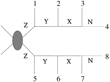
Figure 1: Event topology

Consider the double decay chain in fig. 1. The 4-momenta in the upper chain should satisfy

$$(p_{1}+p_{2}+p_{3}+p_{4})^{2} = m_{Z}^{2}$$

$$(p_{2}+p_{3}+p_{4})^{2} = m_{Y}^{2}$$

$$(p_{3}+p_{4})^{2} = m_{X}^{2}$$

$$p_{4}^{2} = m_{N}^{2}\;.$$ (3)

Defining the mass-squared differences

$$M_{1} = m_{Z}^{2}-m_{Y}^{2}>0$$

$$M_{2} = m_{Y}^{2}-m_{X}^{2}>0$$

$$M_{3} = m_{X}^{2}-m_{N}^{2}>0\;,$$ (4)

the first three equations give linear constraints on the invisible 4-momentum $p_{4}$:

$$-2p_{1}\cdot p_{4} = 2p_{1}\cdot p_{2}+2p_{1}\cdot p_{3}+m_{1}^{2}-M_{1}\equiv S_{1}$$

$$-2p_{2}\cdot p_{4} = 2p_{2}\cdot p_{3}+m_{2}^{2}-M_{2}\equiv S_{2}$$

$$-2p_{3}\cdot p_{4} = m_{3}^{2}-M_{3}\equiv S_{3}\;.$$ (5)

Similarly for the lower chain

$$-2p_{5}\cdot p_{8} = 2p_{5}\cdot p_{6}+2p_{5}\cdot p_{7}+m_{5}^{2}-M_{1}\equiv S_{5}$$

$$-2p_{6}\cdot p_{8} = 2p_{6}\cdot p_{7}+m_{6}^{2}-M_{2}\equiv S_{6}$$

$$-2p_{7}\cdot p_{8} = m_{7}^{2}-M_{3}\equiv S_{7}\;.$$ (6)

We also have the missing transverse momentum constraints

$$p_{4}^{x}+p_{8}^{x} = p^{x}_{\rm miss}\equiv S_{4}$$

$$p_{4}^{y}+p_{8}^{y} = p^{y}_{\rm miss}\equiv S_{8}\;.$$ (7)

If we make an 8-vector of the invisible 4-momenta,

$${\bf P}=(p_{4}^{x},p_{4}^{y},p_{4}^{z},E_{4},p_{8}^{x},p_{8}^{y},p_{8}^{z},E_{8})\;,$$ (8)

then we have

$${\bf AP}={\bf S}$$ (9)

where ${\bf A}$ is the 8$\times$8 matrix

$${\bf A}=2\left(\begin{array}[]{cccccccc}p_{1}^{x}&p_{1}^{y}&p_{1}^{z}&-E_{1}&0&0&0&0\\ p_{2}^{x}&p_{2}^{y}&p_{2}^{z}&-E_{2}&0&0&0&0\\ p_{3}^{x}&p_{3}^{y}&p_{3}^{z}&-E_{3}&0&0&0&0\\ 1/2&0&0&0&1/2&0&0&0\\ 0&0&0&0&p_{5}^{x}&p_{5}^{y}&p_{5}^{z}&-E_{5}\\ 0&0&0&0&p_{6}^{x}&p_{6}^{y}&p_{6}^{z}&-E_{6}\\ 0&0&0&0&p_{7}^{x}&p_{7}^{y}&p_{7}^{z}&-E_{7}\\ 0&1/2&0&0&0&1/2&0&0\end{array}\right)\;.$$ (10)

Furthermore ${\bf S}$ may be written as

$${\bf S}={\bf BM}+{\bf C}$$ (11)

where ${\bf M}=(M_{1},M_{2},M_{3})$ is the 3-vector of mass-squared differences to be determined,

$${\bf B}=\left(\begin{array}[]{ccc}-1&0&0\\ 0&-1&0\\ 0&0&-1\\ 0&0&0\\ -1&0&0\\ 0&-1&0\\ 0&0&-1\\ 0&0&0\end{array}\right)$$ (12)

and

$${\bf C} = (2p_{1}\cdot p_{2}+2p_{1}\cdot p_{3}+m_{1}^{2},2p_{2}\cdot p_{3}+m_{2}^{2},m_{3}^{2},p^{x}_{\rm miss},$$ (13)

$$\;\,2p_{5}\cdot p_{6}+2p_{5}\cdot p_{7}+m_{5}^{2},2p_{6}\cdot p_{7}+m_{6}^{2},m_{7}^{2},p^{y}_{\rm miss})\;.$$

Hence the solution for the invisible 4-momenta is

$${\bf P}={\bf A}^{-1}{\bf S}={\bf DM}+{\bf E}$$ (14)

where ${\bf D}={\bf A}^{-1}{\bf B}$ and ${\bf E}={\bf A}^{-1}{\bf C}$.

The invisible 4-momenta also satisfy the quadratic constraints

$$p_{4}^{2} = P_{4}^{2}-P_{1}^{2}-P_{2}^{2}-P_{3}^{2}=m_{N}^{2}$$

$$p_{8}^{2} = P_{8}^{2}-P_{5}^{2}-P_{6}^{2}-P_{7}^{2}=m_{N}^{2}$$ (15)

where $m_{N}$ is an extra unknown, independent of ${\bf M}$. However, in the case that the terminal pairs of visible decay products (2,3) and (6,7) are opposite-sign same-flavour dileptons, as in (1) or (2), we can reasonably expect that the upper edge of the dilepton invariant mass spectrum will be measured with good accuracy. This quantity is given by

$$(m_{ll}^{\rm max})^{2}\equiv M_{L}=(m_{Y}^{2}-m_{X}^{2})(m_{X}^{2}-m_{N}^{2})/m_{X}^{2}=M_{2}M_{3}/(M_{3}+m_{N}^{2})$$ (16)

and hence

$$m_{N}^{2}=M_{3}(M_{2}/M_{L}-1)\;.$$ (17)

Substituting this into eqs. (2), we obtain a pair of trivariate quadratic equations in $M_{1},M_{2},M_{3}$, whose real solutions lie on a curve in the 3-dimensional space of those variables. The corresponding solutions for the new particle masses are then given by eq. (17) and

$$m_{X}^{2}=m_{N}^{2}+M_{3}\,,\;\;\;m_{Y}^{2}=m_{X}^{2}+M_{2}\,,\;\;\;m_{Z}^{2}=m_{Y}^{2}+M_{1}\;.$$ (18)

The limits $m_{N}^{2}>0$, $m_{Z}^{2}<M_{U}$ (where $M_{U}=s/4$, $s$ being the collider c.m. energy squared, or smaller, depending on the relevant parton luminosities) imply that the solutions must lie within the region

$$0 \leq M_{3} \leq M_{U}-M_{L}$$

$$M_{L} \leq M_{2} \leq M_{U}/(1+M_{3}/M_{L})$$

$$0 \leq M_{1} \leq M_{U}-M_{2}(1+M_{3}/M_{L})\;.$$ (19)

This is a finite region with volume

$$\frac{1}{4}M_{L}\left[2M_{U}^{2}\ln(M_{U}/M_{L})-(3M_{U}-M_{L})(M_{U}-M_{L})\right]\;,$$ (20)

which vanishes as $M_{L}\to 0$ or $M_{L}\to M_{U}$.

3 Results

As an illustration of the method, we apply it here to the process of squark-pair production at the LHC ($pp$ collisions at 14 TeV centre-of-mass energy). The SUSY mass spectrum and decay branching ratios are taken to be those of CMSSM point SPS 1a [7]. The corresponding masses in the decay chain (1) are given in Table 1. Events are generated using HERWIG version 6.5 [8, 9, 10]. Some of the squarks are produced directly and some come from gluino decay; the production mechanism affects their momentum and rapidity distributions but is otherwise irrelevant for our purposes.

$N$	$X$	$Y$	$Z$
$\tilde{\chi}_{1}^{0}$	$\tilde{e}_{R}$	$\tilde{\chi}_{2}^{0}$	$\tilde{u}_{L}$
96	143	177	537

Table 1: Mass spectrum in GeV for Snowmass point SPS 1a

Third-generation squarks are excluded, as their different masses prevent a good fit with a single squark mass. Experimentally, this would involve vetoing events with a tagged $b$-jet. At SUSY point SPS 1a only left-squarks have significant branching ratios into the mode (1) and so the left-right squark mass splitting is not a problem here. The $\tilde{d}_{L}-\tilde{u}_{L}$ mass difference is 5.8 GeV. Therefore the assumption that the masses in the two decay chains are identical should be a good approximation.

To obtain the solution curve for each event, we proceed as follows. As explained earlier, substitution of eq. (17) into eqs. (2) gives a pair of trivariate quadratic equations in $M_{1},M_{2},M_{3}$. Eliminating, for example, $M_{3}$ gives a quartic equation for $M_{2}$ as a function of $M_{1}$. For each real solution, $M_{3}$ is given uniquely in terms $M_{1}$ and $M_{2}$. Thus for each $M_{1}$ we obtain a set of 0, 2 or 4 real solution points. We divide the space of $(M_{1},M_{2},M_{3})$ into cells. Scanning over $M_{1}$ gives a set of solution points which occupy ‘hit’ cells. To find all hit cells we also scan over $M_{2}$ and $M_{3}$, using permutations of the above procedure. Hits on already occupied cells are discarded. The resulting set of points provides an approximately uniform coverage of the solution curve. In general, the solution curve may consist of one or two closed loops or open segments with endpoints on the surface of the allowed region (2).

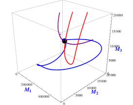
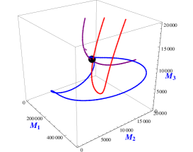
Figure 2: Stereoscopic views of the true parton-level solution curves for three events. The ball shows the true mass point.

Figure 2 shows the parton-level solution curves for three typical SPS1a events, using the correct combinations of quarks and leptons in the decay chains. The curves all pass close to the “true” mass point (TMP)

$$M_{1}=257040\,,\;\;\;M_{2}=10880\,,\;\;\;M_{3}=11233\,,$$ (21)

all in GeV², corresponding to the SUSY mass spectrum in Table 1. The curves do not precisely intersect, even with exact kinematics, owing to Breit-Wigner smearing of unstable particle masses. However, we see that the density of solution curves is high only in the vicinity of the TMP (21).

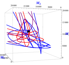
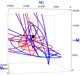
Figure 3: Stereoscopic views of the parton-level solution curves for the same three events, now including all combinations.

Figure 3 shows the effect of combinatorial ambiguities for the same three events, viewed from a different angle for clarity. Here the interchanges of near and far leptons ($2\leftrightarrow 3$ and $6\leftrightarrow 7$) and of quarks ($1\leftrightarrow 5$) are included, making eight combinations per event. Three-dimensional viewing reveals that incorrect combinations either have no real solutions or tend to give curves that do not congregate to form regions of high density.

In the real world, the effects of parton showering, hadronization and detector resolution shift and distort the solution curves. The density of solutions around the TMP is reduced, and incorrect combinations may happen to produce other regions of high density. In addition, QCD radiation produces extra jets, which increase the number of wrong combinations.

To investigate these effects, we study an inclusive SUSY sample containing SUSY backgrounds as well as signal processes, generated using HERWIG 6.5 with initial and final state radiation turned on. The sample is interfaced with AcerDET 1.0 [11]. Final-state hadrons are formed into jets, and the momenta of jets and leptons are smeared according to the simulated detector resolution.

	$m_{0}$	$m_{1/2}$	$A_{0}$	$\tilde{\chi}_{1}^{0}$	$\tilde{e}_{R}$	$\tilde{\chi}_{2}^{0}$	$\tilde{u}_{L}$
Point A	110	220	0	86	142	161	504
Point B	100	250	$-100$	99	141	186	563
Point C	140	260	0	103	174	193	592

Table 2: Parameters and mass spectra in GeV for non-CMSSM model points A, B and C. Parameters common to all points are $m_{0}^{\rm 3rd\,gen.}=300$ GeV, $\tan\beta=10$, ${\rm sign}(\mu)=+$.

To obtain a larger event sample with two decay chains like (1), for this analysis we adopt non-CMSSM model points A, B and C, where the third-generation soft mass is larger than the others, so that the branching ratio (1) is increased by suppressing the $\tilde{\chi}_{2}^{0}\to\tilde{\tau}_{1}^{\pm}\tau^{\mp}$ mode. The sparticle spectra at these points are shown in Table 2. The generated samples of 500,000 events correspond to about 10, 15 and 20 ${\rm fb}^{-1}$ of integrated luminosity, respectively.

The following cuts are applied in order to select signal events:

(i)

$M_{\rm eff}\equiv\sum_{i=1}^{4}p_{T}^{{\rm jet},i}+\sum_{i=1}^{4}p_{T}^{{\rm lep},i}+E_{T}^{\rm miss}>400\,{\rm GeV}$  ;

(ii)

$E_{T}^{\rm miss}>\max(200\,{\rm GeV},~{}0.2M_{\rm eff})$ ;

(iii)

At least two jets with $p_{T}^{{\rm jet},1}>100\,{\rm GeV}$ and $p_{T}^{{\rm jet},2}>50\,{\rm GeV}$ within $|\eta|<2.5$ ;

(iv)

Two pairs of opposite sign same flavour leptons with $p_{T}>20\,{\rm GeV}$ and $|\eta|<3$ ;

(v)

No $b$ jet with $p_{T}>30\,{\rm GeV}$ and $|\eta|<3$ .

The $b$ tagging efficiency is assumed to be $60\%$. In the cut (iv), we select not only opposite-flavour lepton pairs ($e^{+}e^{-}\mu^{+}\mu^{-}$) but also the same-flavour pairs ($e^{+}e^{-}e^{+}e^{-}$ and $\mu^{+}\mu^{-}\mu^{+}\mu^{-}$) to have larger samples, although the latter have double the combinatorial background of the former. If an event contains more than two hard jets, we take the three hardest jets as candidates for the jets from the signal decay chains (1), and try all possible combinations. The number of combinations is 8 (16) for two candidate jets and 24 (48) for three with opposite (same) flavour lepton pairs. The numbers of events that survive the above cuts are shown in the first row in Table 3 together with signal/background ratios for each model point. The background is rather mixed, coming mainly from direct $\tilde{\chi}_{2}^{0}$ productions associated with squarks or gauginos as well as modes containing $\tilde{q}_{R}\to\tilde{\chi}_{2}^{0}j$, $\tilde{b}_{1}\to\tilde{\chi}_{2}^{0}b$ and $\tilde{\chi}_{2}^{0}\to\tilde{\chi}_{1}^{0}l^{+}l^{-}$. For model point C, the three-body decay $\tilde{\chi}_{2}^{0}\to\tilde{\chi}_{1}^{0}l^{+}l^{-}$ is enhanced because $m_{\tilde{\chi}_{2}^{0}}\simeq m_{\tilde{\chi}_{1}^{0}}+m_{Z}$ and turns out to be the main background. Standard Model background is expected to be negligible after the above selection cuts. According to ref. [12], the potential background comes from $t\bar{t}\to b\bar{b}W^{+}W^{-}\to 4l$. Based on HERWIG 6.5 simulation of this process, we confirmed that it is indeed negligible after cuts.

	Point A	Point B	Point C
Events (S/B)	326 (4.2)	499 (4.5)	292 (2.8)
Sharing (S/B)	219 (8.1)	341 (9.7)	172 (4.9)
$M_{1}$ (True ; Best)	231890 ; $222500$	286157 ; $282500$	316274 ; $317500$
$M_{2}$ (True ; Best)	5624 ; $5000$	14520 ; $14200$	6815 ; $6600$
$M_{3}$ (True ; Best)	12872 ; $11700$	10293 ; $9900$	19812 ; $18900$

Table 3: First row: number of events (signal/background) after cuts. Second row: number of events that contribute to the best-fit cell in the $\Delta\chi^{2}$ distribution. Third to fifth rows: true mass and the central value of the best-fit cell in $\rm GeV^{2}$.

If the detector and jet properties are well understood, from the observed jet momentum, $p^{\rm jet}$, we may stochastically estimate the original parton momentum, $p^{\rm par}$, with a gaussian distribution $\epsilon(p^{\rm par}|p^{\rm jet})$. In this situation, we can built a confidence region in the ($M_{1}$, $M_{2}$, $M_{3}$) space [4]. For each signal event combination, $i_{\rm ev}$, a probability density function may be constructed as

$$f_{i_{\rm ev}}({\bf M})=\frac{1}{N_{i_{\rm ev}}}\int dp^{\rm par}_{1}dp^{\rm par}_{2}\epsilon(p^{\rm par}_{1}|p^{\rm jet}_{1})\epsilon(p^{\rm par}_{2}|p^{\rm jet}_{2})\delta(p_{4}^{2}-m^{2}_{N})\delta(p_{8}^{2}-m^{2}_{N}),$$ (22)

where $p_{4}$, $p_{8}$ and $m_{N}$ are the functions of ${\bf M}$ and $p^{\rm par}_{1,2}$ given in section 2, and $N_{i_{\rm ev}}$ is a normalization factor. Given $N$ event-combinations, log-likelihood and $\Delta\chi^{2}$ functions are obtained as

$$\ln L({\bf M})=\sum_{i_{\rm ev}}^{N}\ln f_{i_{\rm ev}}({\bf M})$$ (23)

and

$$\Delta\chi^{2}({\bf M})=2(\ln L({\bf M})_{\rm max}-\ln L({\bf M})),$$ (24)

respectively, where $\ln L({\bf M})_{\rm max}$ is the maximum value of $\ln L({\bf M})$ in the space ${\bf M}$.

We calculate $\ln L({\bf M})$ approximately by the following procedure. For each event, we generate Monte Carlo “fake” events whose jet momenta are shifted from the original ones according to the probability distribution $\epsilon(p^{\rm par}|p^{\rm jet})$. The parameter space ${\bf M}$ is divided into cells. For each cell, we count the number of fake events for which the solution curves go through that cell. If different combinations of the same event yield two or more curves passing through the same cell, we count only one. If the number of fake events is large and the cell size is small, this provides $f_{i_{\rm ev}}({\bf M}_{\rm cell})$ with a certain normalization. As long as we work with $\ln L({\bf M})$, the normalization factor $N_{i_{\rm ev}}$ is irrelevant, because it only shifts the constant term of $\ln L({\bf M})$. We ignore cells that have $f_{i_{\rm ev}}({\bf M}_{\rm cell})=0$ in our log-likelihood calculation, setting $\ln f_{i_{\rm ev}}({\bf M}_{\rm cell})=0$. Finally, we sum up $\ln f_{i_{\rm ev}}({\bf M}_{\rm cell})$ for all combinations of all events.

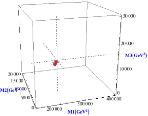
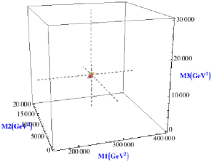
(A)     (B)      (C)

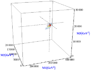
Figure 4: Distribution of $\Delta\chi^{2}({\bf M})$ for each model point at detector level. The true mass point is at the intersection of the three dashed lines.

In the following analysis, we generate 1000 Monte Carlo fake events for each event. For the smearing of jets and the missing transverse momentum, we use gaussian functions with the following standard deviations, obtained by parametrizing the AcerDET results:

$$\frac{\sigma_{E}}{E}=\frac{0.5}{\sqrt{E}}+0.03,~{}~{}~{}~{}~{}\sigma_{\phi}=\frac{0.4}{\sqrt{E}}+0.015,~{}~{}~{}~{}~{}\sigma_{\eta}=\frac{0.3}{\sqrt{E}}+0.02,$$ (25)

for jets and

$$\frac{\sigma_{E}}{E}=\frac{0.5}{\sqrt{E}}+0.03,~{}~{}~{}~{}~{}~{}\sigma_{\phi}=\frac{0.8}{\sqrt{E}}+0.06,$$ (26)

for the missing transverse momentum. We do not smear the lepton momenta because mismeasurement of lepton momenta is negligible compared to the jet smearing.

Figure 4 shows the $\Delta\chi^{2}({\bf M})$ distribution obtained by the above procedure for each model point. The cell size is $\Delta M_{1}=5000$, $\Delta M_{2}=400$, $\Delta M_{3}=600$ in ${\rm GeV}^{2}$. The distribution has only one sharp minimum, which is close to the TMP, as can be seen in Table 3. Backgrounds from wrong combinations and different decay chains do not produce local minima at other places, and the effect of those backgrounds may be less significant around the true mass point.

The second row in Table 3 shows how many different events share the best-fit cell; the signal/background ratios in that cell are also shown in parentheses. The ratios are improved significantly. For each model point the ratio is about twice that for the whole sample.

	$\tilde{\chi}_{1}^{0}$	$\tilde{e}_{R}$	$\tilde{\chi}_{2}^{0}$	$\tilde{u}_{L}$
Point A	$68.2^{+16.2}_{-5.8}$	$127.9^{+12.6}_{-4.2}$	$146.1^{+13.0}_{-4.4}$	$493.8^{+11.5}_{-3.8}$
Point B	$94.5^{+8.5}_{-2.8}$	$137.2^{+9.1}_{-3.1}$	$181.7^{+8.5}_{-2.8}$	$561.7^{+9.4}_{-3.1}$
Point C	$95.6^{+5.1}_{-5.3}$	$167.4^{+3.9}_{-3.9}$	$186.1^{+4.0}_{-4.0}$	$593.4^{+3.4}_{-3.4}$

Table 4: Estimated sparticle masses with their errors in GeV.

In the third to fifth row of Table 3, we show the central values of the best-fit cells compared to the TMP at each model point. As can be seen, the best-fit points are slightly biased towards lower masses. This may result from the following systematic errors in the present analysis. First, the AcerDET jets that we use are defined as massless, whereas the 4-momenta defined by $p^{\rm par}=p(\tilde{q})-p(\tilde{\chi}^{0}_{2})$ have masses of around 10-100 GeV after fragmentation and hadronization. Second, we have parametrized the probability distributions of parton momenta by gaussian functions. However, the difference between a parton momentum in the event record and the AcerDET jet momentum deviates slightly from a gaussian distribution, due to the underlying event, hadronization effects and high-$p_{T}$ gluon emission from the original parton. A better jet algorithm with jet masses and a more refined parametrization will be needed to reduce these systematic errors.

Table 4 shows the sparticle masses estimated from our analysis. The errors are obtained from $1\sigma$ regions assuming the errors in $M_{1}$, $M_{2}$ and $M_{3}$ are uncorrelated, where the $1\sigma$ region is defined by $\Delta\chi^{2}<3.53$. We neglect the error from the mismeasurement of the dilepton endpoint because of its expected good accuracy. The $1\sigma$ errors at Point C are accidentally small despite the small number of signal events compared to the other points. The sizable errors also come from the cell size, because the $1\sigma$ region is almost the same size as the cells. More precise error estimation would require smaller cells. In addition, larger numbers of fake Monte Carlo events could be used to make the probability density smooth around the peak region. Such refinements would be justified and straightforward in an analysis of real data.

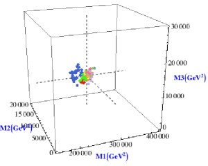
(A)   (B)    (C)

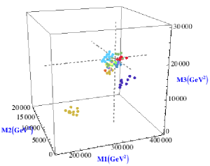
Figure 5: One-sigma regions of 10 sub-samples, distinguished by their colours. Each sub-sample contains 25 events.

The statistical approach we have adopted here is justifiable for large event samples. In order to see what happens in small samples, and to check the interpretation of $\Delta\chi^{2}$, we divide the samples after cuts into several sub-samples, so that each of them contains 25 events. Figure 5 shows the $1\sigma$ regions of 10 sub-samples for each model point. The sub-samples are distinguished by their colours. As expected, the $1\sigma$ regions are more widely spread compared to Figure 4. As can be seen in Figure 5 C, the gold-coloured sub-sample has two local minima, one of them away from the TMP. Furthermore, the $1\sigma$ region of the blue-coloured sub-sample is localised away from the TMP. Those sub-samples have fewer signal events compared to the others. The signal/background ratio is 1.8 (2.6) for the blue (gold) sub-sample. We checked, however, that the $2\sigma$ region of the blue sub-sample contains the TMP. Despite the small sub-sample sizes, the maximum-likelihood regions are still mainly localised around the TMP, and their average sizes scale as expected with the number of events. In our approach, unlike in endpoint and kink methods, all signal events contribute to the determination of the unknown masses, no matter where they may lie in phase space, and so the method can provide meaningful information about the unknown masses even in rather small samples.

4 Conclusions

The method of mass determination presented above is simple to apply and looks promising for the class of processes studied here. We demonstrated the validity of the method by means of full simulations including detector effects. Combinatorial background, the background from other SUSY processes and the effects of additional jets due to QCD radiation do not appear to be a serious problem. A statistical approach is applicable to deal with jet momentum mismeasurement. We constructed an effective $\Delta\chi^{2}$ variable which allows a rather precise determination of the unknown masses with controlled statistical errors. There are identified systematic errors, leading to a bias towards lower masses, which could be reduced with an appropriate jet algorithm and improved parametrization of jet momentum smearing. The method can be applied successfully even to small event samples, because it makes full use of the kinematical information from every event.

Note added: The procedure adopted here for constructing an approximate likelihood function by generating large numbers of “fake” events is quite time-consuming. An analytical procedure similar to that outlined (but not implemented) for the exact-solution method in Section 6 of ref. [3] may be applicable and more efficient. We thank H. C. Cheng for this suggestion.

Aknowledgements

KS and BW are grateful for helpful discussions with other members of the Cambridge SUSY Working Group. BW thanks the CERN Theory Group for hospitality during part of this work.

References

- [1] A. J. Barr and C. G. Lester, “A Review of the Mass Measurement Techniques proposed for the Large Hadron Collider,” arXiv:1004.2732.
- [2] H. C. Cheng, D. Engelhardt, J. F. Gunion, Z. Han and B. McElrath, “Accurate Mass Determinations in Decay Chains with Missing Energy,” Phys. Rev. Lett. 100 (2008) 252001 [arXiv:0802.4290 [hep-ph]].
- [3] H. C. Cheng, J. F. Gunion, Z. Han and B. McElrath, “Accurate Mass Determinations in Decay Chains with Missing Energy: II,” Phys. Rev. D 80 (2009) 035020 [arXiv:0905.1344 [hep-ph]].
- [4] K. Kawagoe, M. M. Nojiri and G. Polesello, “A new SUSY mass reconstruction method at the CERN LHC,” Phys. Rev. D 71 (2005) 035008 [arXiv:hep-ph/0410160].
- [5] M. M. Nojiri, G. Polesello and D. R. Tovey, “A hybrid method for determining SUSY particle masses at the LHC with fully identified cascade decays,” JHEP 0805 (2008) 014 [arXiv:0712.2718 [hep-ph]].
- [6] B. Webber, “Mass determination in sequential particle decay chains,” JHEP 0909, 124 (2009) [arXiv:0907.5307 [hep-ph]].
- [7] B. C. Allanach et al., “The Snowmass points and slopes: Benchmarks for SUSY searches,” in Proc. of the APS/DPF/DPB Summer Study on the Future of Particle Physics (Snowmass 2001) ed. N. Graf, Eur. Phys. J. C 25 (2002) 113 [arXiv:hep-ph/0202233].
- [8] G. Corcella et al., “HERWIG 6.5: an event generator for Hadron Emission Reactions With Interfering Gluons (including supersymmetric processes),” JHEP 0101 (2001) 010 [arXiv:hep-ph/0011363].
- [9] G. Corcella et al., “HERWIG 6.5 release note,” arXiv:hep-ph/0210213.
- [10] S. Moretti, K. Odagiri, P. Richardson, M. H. Seymour and B. R. Webber, “Implementation of supersymmetric processes in the HERWIG event generator,” JHEP 0204, 028 (2002) [arXiv:hep-ph/0204123].
- [11] E. Richter-Was, “AcerDET: A particle level fast simulation and reconstruction package for phenomenological studies on high p(T) physics at LHC,” arXiv:hep-ph/0207355, http://erichter.home.cern.ch/erichter/AcerDET.html
- [12] G. L. Bayatian et al. [CMS Collaboration], “CMS technical design report, volume II: Physics performance,” J. Phys. G 34 (2007) 995.