Validation of frequency and mode extraction calculations from time-domain simulations of accelerator cavities

Abstract

The recently developed frequency extraction algorithm [G. R. Werner and J. R. Cary, J. Comp. Phys. 227, 5200 (2008)] that enables a simple FDTD algorithm to be transformed into an efficient eigenmode solver is applied to a realistic accelerator cavity modeled with embedded boundaries and Richardson extrapolation. Previously, the frequency extraction method was shown to be capable of distinguishing $M$ degenerate modes by running $M$ different simulations and to permit mode extraction with minimal post-processing effort that only requires solving a small eigenvalue problem. Realistic calculations for an accelerator cavity are presented in this work to establish the validity of the method for realistic modeling scenarios and to illustrate the complexities of the computational validation process. The method is found to be able to extract the frequencies with error that is less than a part in 10⁵. The corrected experimental and computed values differ by about one parts in 10⁴, which is accounted for (in largest part) by machining errors. The extraction of frequencies and modes from accelerator cavities provides engineers and physicists an understanding of potential cavity performance as it depends on shape without incurring manufacture and measurement costs.

I Introduction

Once a computational application has been verified (shown to correctly solve the mathematical model of a physical system), for confidence in modeling, the application needs to be validated, i.e., shown to accurately represent the physical systems of interest. Inevitably, validation is a process of determining the causes of discrepancies between computational and experimental results. This paper focuses on validation of frequency and mode extraction computations of accelerator cavities using time-domain simulations. The calculations are based on the novel method of Werner and Cary which employs time-domain simulations of Maxwell’s equations using the finite-difference time-domain (FDTD) method Werner and Cary (2008). The Werner-Cary method has been shown to permit extraction of degenerate frequencies and to provide the ability to reconstruct the modes using only a minimal amount of post-processing linear algebra.

The common approach to frequency extraction for time-domain simulations of Maxwell’s equations using the FDTD method is to compute narrowly-filtered states. A narrowly-filtered state can be computed using a square window that excites only those modes around a desired frequency, $\omega$. In Maxwell’s equations, this equates to the sinusoidal excitation $f(t)=W(t)\sin(\omega t)$ where $W(t)=\Theta(t)\Theta(t-T)$ given that $\Theta(t)$ is the Heaviside function. One can also excite a broad range in a similar way and then perform post-simulation FFTs on the broadly-filtered states to determine the frequencies of the system. Such methods, however, do not provide a means for constructing the eigenmodes or for handling degeneracies.

We apply the Werner-Cary method to a realistic accelerator cavity that was fabricated at Fermi National Accelerator Laboratory (Fermilab) in 1999. The method is applied to calculations performed with the VORPAL computational framework Nieter and Cary (2004). Previous analysis of this cavity shape had been carried out using the MAFIA code (cf. M. Clemens et al. (1999)), with stair-step and diagonal boundaries and cylindrical symmetry McAshan and Wanzenberg ; Bellantoni . Accelerator cavities are an essential component of large collider experiments like the Large Hadron Collider. The shape, curvature, and size of these cavities determine the performance of the cavities; simulations are important in the designing of these cavities to maximize performance and minimize design error. We show the ability to get frequencies accurate to less than a part in $10^{5}$.

The complexities of the validation process will be focused on here as we illustrate the process that was undertaken to determing the causes for discrepancies between computational and experimental results. Our requirement for validation is that the discrepancies are reduced to measurement and/or computational uncertainties. In the present case, we show that the discrepancies are due to both computational error and error associated with the cavity dimensions. The latter has two aspects. The first is that cavities cannot be fabricated precisely to specifications, and so one must do a post-fabrication measurement of the cavity dimensions. The second is that even those post-fabrication measurements have associated uncertainties. For the particular case shown here, it is found that the greatest uncertainties derive from the uncertainties in cavity dimensions. The computational error is smaller by a few orders of magnitude. This is not too surprising, in that accelerator cavities are not primarily designed to have low frequency sensitivity with respect to mechanical dimensions. Nevertheless, this shows how realistic frequency sensitivities are taken into account in a validation study.

We begin with a review of the broadly-filtered diagonalization method presented in Ref. Werner and Cary (2008). We then introduce the A15 accelerator cavity built at Fermilab. We describe the details of the cavity and previous work on extracting frequencies and modes of this cavity. The subsequentsection discusses our frequency computations from the specified dimensions and their comparison with the measurements. We also consider resolution of the observed differences, showing that dimensional uncertainties are dominant. We then present work on how modes can be obtained using the Broadly-Filtered Filter Diagonalization Method. We finally summarize and conclude.

II Broadly-Filtered FDM

The Broadly-Filtered Filter Diagonalization Method (FDM) introduced in Ref. Werner and Cary (2008) is an extension of the concepts presented in Refs. Neuhauser (1990, 1994); Wall and Neuhauser (1995); Mandelshtam and Taylor (1997); Mandelshtam (2003). We review the method in terms of linear operator ${\cal L}$ that represents a discrete $\nabla\times\nabla\times$ generated by the Yee method Yee (1966). The field of interest, ${\bf s}$, is the elecric field, ${\bf E}$, or the magnetic field, ${\bf B}$. If we view Maxwell’s equation in the second-order form

$$-\frac{1}{c^{2}}\frac{\partial^{2}}{\partial t^{2}}{\bf E}(x,y,z,t)=\nabla\times\nabla\times{\bf E}(x,y,z,t)={\cal L}{\bf E}(x,y,z,t),$$ (1)

then the eigenvalue problem for $\nabla\times\nabla\times$ can be seen as a time evolution problem, relating eigenvalues to frequencies.

The broadly-filtered FDM is based on the idea that the linear operator, ${\cal L}$, can be transformed into block-diagonal form with one large block filtered out and the remaining small block diagonalized by the singular value decomposition (SVD). The majority of the work goes into the diagonalization, which requires finding a small, invariant subspace of the field of interest. We generate this invariant subspace using a frequency filtering method based on targeted excitations of Maxwell’s equations using a current density that is geared towards the frequencies of interest. See Eq. (13).

The filtering is with respect to a FDTD discretization of Maxwell’s equations for which the current source ${\bf J}(x,y,z,t)$ excites the electric and magnetic fields according to

$$\begin{array}[]{rcl}\frac{\partial\mathbf{B}(x,y,z,t)}{\partial t}&=&-\nabla\times\mathbf{E}(x,y,z,t)\\ \frac{1}{c^{2}}\frac{\partial\mathbf{E}(x,y,z,t)}{\partial t}&=&\nabla\times\mathbf{B}(x,y,z,t)-\mu_{0}\mathbf{J}(x,y,z,t).\end{array}$$ (2)

The current is defined as $\mathbf{J}(x,y,z,t)=f(t)\hat{\mathbf{J}}(x,y,z)$ where

$$f(t)=\left\{\begin{array}[]{lc}2\left[\frac{\sin(\omega_{1}(t-T/2))}{t-T/2}-\frac{\sin(\omega_{2}(t-T/2))}{t-T/2}\right]\exp^{-\sigma_{\omega}^{2}(t-T/2)^{2}/2}&0\leq t\leq T,\\ 0.&\mathrm{otherwise}\end{array}\right.$$ (3)

$\hat{\mathbf{J}}(x,y,z)$ has a pattern that encourages excitation of the desired modes in the frequency range $[\omega_{1},\omega_{2}]$. The parameter $\sigma_{\omega}$ is determined by the separation of the frequencies in $[\omega_{1},\omega_{2}]$ from the next nearest frequency value. If $\hat{\omega}<\omega_{1}$ is the nearest frequency, then

$$\sigma_{\omega}<\frac{|\omega_{1}-\hat{\omega}|}{5.68}$$ (4)

and

$$T>\frac{11.4}{\sigma_{\omega}}$$ (5)

ensures that $\hat{\omega}$ and all other outside modes are suppressed by at least O($1e$-$7$). Here, we have used the frequency amplitude of a Gaussian-modulated sinusoid.

If a $K$-degeneracy is known a priori to exist, then $K$ different spatial currents, $\hat{\mathbf{J}}$, are used yielding $K$ simulations to extract the $K$-degeneracy. The $K$spatial currents should be chosen with an understanding of the symmetry of the cavity and the degenerate modes.

After the excitation is completed, the fields are temporally sampled at random grid points and then can be represented as a linear combination of the desired modes. We then use this knowledge to extract the desired frequencies and spatial mode patterns. To see this, consider the eigenvalue problem, ${\cal L}\mathbf{v}_{m}=\lambda_{m}\mathbf{v}_{m}$, and the discrete fields, $\mathbf{s}_{\ell}$, sampled in time. If we define

$$\mathbf{r}_{\ell}={\cal L}\mathbf{s}_{\ell}$$ (6)

and use the fact that any eigenvector $\mathbf{v}_{m}$ can be expressed as a sum over the temporal samples according to

$$\mathbf{v}_{m}=\sum_{\ell=1}^{L}a_{m,\ell}\mathbf{s}_{\ell},$$ (7)

then applying ${\cal L}$ yields

$$\lambda_{m}\mathbf{v}_{m}=\sum_{\ell=1}^{L}a_{m,\ell}\mathbf{r}_{\ell}.$$ (8)

Since we have $\mathbf{s}_{\ell}$ and $\mathbf{r}_{\ell}$, Eqs. (7) and (8) can be solved for the $\lambda_{m}$ (the eigenvalues) and the coefficients $a_{m,l}$ (allowing us to contruct the eigenvectors).

In practice, we only work with $P$ randomly-sampled spatial components of the fields yielding the generalized eigenvalue problem

$$R\mathbf{a}_{m}=\lambda_{m}S\mathbf{a}_{m},$$ (9)

where the number of colums of $R$ and $S$ correspond to the number of temporal samples and the number of rows correspond to the number of spatial samples. Eq. (9) can only be solved when $S$ is invertible, which requires $L=P$. In general, we prefer $P>2L$ implying we must solve the generalized eigenvalue problem

$$S^{\dagger}R\mathbf{a}_{m}=\lambda_{m}S^{\dagger}S\mathbf{a}_{m},$$ (10)

using the SVD for $S^{\dagger}S=VD^{2}V^{\dagger}$, where $D$is diagonal and $V$ is orthogonal. Since $S^{\dagger}S$ may be singular, $D$ may have zeros on the diagonal, so we construct $\tilde{D}$ such that

$$\tilde{D}^{-1}_{\ell\ell}=\left\{\begin{array}[]{cl}D^{-1}_{\ell\ell}&\frac{D_{\ell\ell}}{D_{\mathrm{max}}}>\alpha_{\mathrm{cutoff}}\\ 0&\frac{D_{\ell\ell}}{D_{\mathrm{max}}}\leq\alpha_{\mathrm{cutoff}}\end{array}\right.$$

where $\alpha_{\mathrm{cutoff}}$ is a small value chosen to distinguish significant diagonal values from the insignificant diagonal values. We then solve the eigenvalue problem

$$V(\tilde{D})^{-2}V^{\dagger}S^{\dagger}\,R\mathbf{a}_{m}=\lambda_{m}\mathbf{a}_{m},$$ (11)

computing the eigenvalues $\lambda_{m}$. The coefficients, $\mathbf{a}_{m}$, are then used to construct the field pattern, i.e., the eigenmode, by using Eq. (7). We refer the reader to Ref. Werner and Cary (2008) for further details.

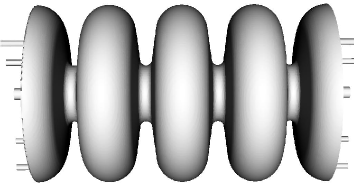
(a)  Side View

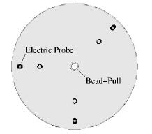
(b)  End-on View

Figure 1: A Side (a) and End-on (b) view of the A15 cavity. The center hole in the End-on view labeled Bead-Pull was used for bead-pull experiments and the smaller off-center endplate hole labeled Electric Probe held an electric probe that created a dipole perpendicular to the page.

III A15 Cavity

In Ref. Werner and Cary (2008) thirteen TM modes in a rectangular 2D cavity were found using the frequency extraction algorithm. The standard Yee method was used to discretize Maxwell’s equations and to evolve the electric and magnetic fields Yee (1966). Here, validation is performed for an extensively tested stack of four unpolarized dumbbells from Fermilab. We refer to this stack, which is pictured in Fig. 1, as the A15 cavity.

The A15 cavity was designed in 1999 for the development of a separated K⁺ beam Bellantoni et al. (2001). It is a deflecting mode cavity designed to operate at 3.9 GHz, i.e., the $\pi$ mode. The cavity shape is determined by parameters such as the equatorial radius ($b$), iris radius ($a$), iris curvature ($r_{i}$), equatorial curvature ($r_{e}$), and cell half length ($g/2)$, displayed schematically in Fig. 2. For the A15 cavity, these parameters are 47.19 mm, 15.00 mm, 3.31 mm, 13.6 mm, and 19.2 mm.

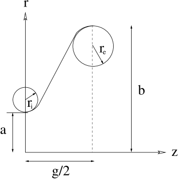
Figure 2: Schematic of the A15 cavity describing the shape in relation to the equatorial radius ($b$), the iris radius ($a$), the iris curvature ($r_{i}$), the equatorial curvature ($r_{e}$), and the cell half length ($g/2)$

The endplate holes observed in the end-on view of Fig. 1 were used for experimental purposes. The large center hole positioned on the centerline of the cavity (radius=3.175 mm) was used for bead-pull experiments. One of the off-center holes (radius=1.5875 mm) provided space for an electric probe that created a dipole. Furthermore, an equivalent set of holes exists on the other endplate. Cavities used within working accelerators would be without these holes; however, these holes only have a small effect on frequencies (tens of kHz) and validation.

In Ref. Bellantoni the frequencies of the A15 cavity were reported from bead-pull experiments. The frequencies were corrected for temperature, barometic pressure, and relative humidity to the frequency that would be measured in a vacuum at 25^∘ C yielding the values presented in Table 1. In addition to the TM₁₁₀ modes, Ref. Bellantoni also had frequencies for the TM₀₁₀ modes as well as other higher-order modes.

	$f_{0}$	$f_{1}$	$f_{2}$	$f_{3}$	$f_{4}$
Exact	3902.810	3910.404	3939.336	4001.342	4106.164
Computed	3900.512	3908.552	3937.325	4000.107	4103.616

Table 1: The first line is the set of frequencies (in MHz) of the five deflecting modes for the A15 cavity. Measurements were performed at Fermi National Accelerator Laboratory in 2000 by Bellantoni et al. and presented in the unpublished note Bellantoni . The second line is the initial set of computations using the original specifications in Bellantoni and discussed in the section Frequency Calculations.

Applying the broadly-filtered FDM to the A15 cavity requires boundary methods that approximate Maxwell’s equations on the cells cut by the cavity boundary. We used the Dey-Mittra method Dey and Mittra (1997) for solving Maxwell’s equations on the cavity’s curved boundaries. The Dey-Mittra method requires that one exclude small fractional areas, with the exclusion depending on the ratio $f_{DM}\equiv\Delta t/\Delta t_{CFL}$ of simulation time step to the CFL time step of a system without embedded boundaries. A method for choosing which areas are excluded that guarantees numerical stability is discussed in Nieter et al. (2009). For our simulations, we used $f_{DM}=0.1$.

IV Frequency Calculations

Previously, we described how the frequency filtering approach for Maxwell’s equation involved selecting an appropriate time-varying current that selectively excites a given frequency range. Defining $f_{L}=$ 3902 MHz and $f_{U}=$ 4110 MHz, the frequency filtering aproach requires knowledge of the separation between $[f_{L},f_{U}]$ and the nearby modes. From Ref. Bellantoni it was known that the mode nearest to the range was the mode at $f_{b}=$ 4320 MHz. When previous calculations or experiments are not available, a few quick simulations followed by FFTs can identify rough locations of modes.

To reduce this nearest unwanted mode by $h=1e$-$7$, we must run the excitation for at least 200 oscillations at $4000$ MHz, since

$$fT=\frac{32}{\pi}\frac{f}{|f_{b}-f_{U}|}.$$ (12)

See Ref. Werner and Cary (2008) for details. This suppresses modes more than 200 MHz away from $f_{U}$, i.e., frequencies above 4310 MHz. Adding the time for sampling of $\pi/|f_{b}-f_{U}|$ the total number of oscillations is approximately 260 oscillations.

We have also judiciously chosen the spatial pattern, $\hat{\mathbf{J}}(x,y,z)$, using a priori knowledge of the modes of interest. When there is no known spatial pattern, the user can create a random pattern for $\hat{\mathbf{J}}$. For the A15 cavity, we used the spatial pattern given by

$$\hat{J}_{x}(x,y,z):=j_{T}(y,z)\,[a_{1} \cos(2kx)+a_{2}\cos(4kx)+b_{1}\cos(kx)$$ (13)

$$+b_{2}\sin(3kx)+b_{3}\sin(kx)]$$

where $k=\pi/0.1536$, $j_{T}(y,z)=y$ or $z$, and $\hat{\mathbf{J}}=(\hat{J}_{x},\hat{J}_{y},\hat{J}_{z})^{T}$. The coefficients $a_{m}$ and $b_{n}$ are chosen at random for a given simulation, thus running multiple simulations to properly account for the two polarizations split by only a few kHz at each frequency value just requires that we have random coefficients for each simulation.

We computed the frequencies for different cell sizes. In all cases, we used $\Delta y=\Delta z=1.25\Delta x$, where $x$ denotes the longitudinal coordinate. The cell size $\Delta x$varied from 0.533 mm to 0.267 mm implying that the cell sizes, $\Delta y$, and $\Delta z$, vary from 0.666 mm to 0.333 mm, thus resolving the hole sizes of 3.175 mm and 1.5875 mm. At the given resolutions and the given Dey-Mittra fractional face parameter, it was observed that the Yee method combined with the Dey-Mittra boundary algorithm was second-order.

Since the method was second-order, Richardson extrapolation could be used to achieve a third-order method, i.e., one makes the assumption,

$$\omega_{i}\sim\omega_{0}+\alpha/N_{i}^{2},$$ (14)

where $\omega_{i}$ is the $i^{th}$ computed frequency, $\omega_{0}$ is the true frequency, $N_{i}$ is the number of cells across the simulations in any particular direction (given that all directions are refined together) for that computation, and $\alpha$ is the error coefficient. Using two computed frequencies at two different resolutions, one gets two equations generated from Eq. (14) for both $\omega_{0}$ and $\alpha$. Given more than two points, one can also determine the frequency from a regression analysis. Using these multiple means of extraction to compute the frequency and then finding the standard deviation of the mean of those results, we were able to deduce that the computational error was $O(10-40)$ kHz for the range of frequencies. That is, the modes can be found to an accuracy that is less than a part in $10^{5}$.

In Fig. 3, we have plotted the convergence of computed frequencies and the value obtained with Richardson extrapolation as an unfilled circle on the ordinate axis. Also shown on the ordinate axis are the experimental values presented in Ref. Bellantoni . Note that there are two polarizations at each frequency value with a slight split in the values. These values differ by anywhere from 3-6 kHz. An averaged value has been used in the plots and in the Richardson extrapolated values.

In Fig. 4, we have plotted a slice of the $E_{x}$ component in the $yz$-plane for one of the two polarizations of the $\pi$ mode. We have produced this plot for various rotations about the longitudinal direction of the cavity in the computational domain the method’s ability to capture the dependency of the splitting of the polarizations on the endplate holes and not the grid. The polarization that is not shown was orthogonal to the one in the figure. When no endplate holes are used, the two polarizations are still orthogonal but their configuration is based on the transverse components of the currents used to excite the modes, i.e. Eq. (13).

Figure 3: Convergence plot (f_CN) of the frequencies of the five deflecting modes for the cavity with the dimensions specified in Ref. Bellantoni . The abscissa represents the grid resolution and the ordinate corresponds to the frequency value in MHz. Each plot has on the ordinate the experimental values (f_EN) from Table 1 for reference purposes and the Richardon’s extrapolated values as unfilled circles.

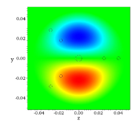
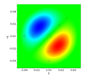
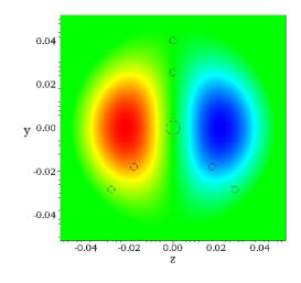
Figure 4: Slice of the $E_{x}$ component for one of the two polarizations of the $\pi$ mode for the various rotations in the computational domain of the cavity. The other polarization was orthogonal to the one shown and the difference in frequency between the two polarizations was only a few kHz. Also to be noted is the arrangement of the polarization due to the endplate hole alignment.

From Fig. 3 the discrepancies between the computed and measured values are apparent. The values obtained with Richardson extrapolation are also presented numerically in Table 1. They are seen to differ from the experimental measurements in Table 1 by 1.5–2.5 MHz. This difference significantly exceeds the computational uncertainty. Hence, we must understand the origin of the difference.

V Validation: resolution of differences

The differences (1.5–2.5 MHz) between the computed values and the experimentally measured values of Table 1 exceed the estimated computational uncertainty; in this section we describe how we resolved these differences. We began by considering possible sources of the discrepancy: computational error, missing physics in the simulation, and cavity (geometry) measurement error.

Figure 5: Convergence plot ($\mathrm{f}_{\mathrm{C}N}$) of the frequencies of the five deflecting modes. The abscissa represents the grid resolution and the ordinate corresponds to the frequency value in MHz. Each plot has on the ordinate the experimental values (f_EN) from Table 1 for reference purposes as well as the Richardson extrapolated values as unfilled circles. The geometrical measurements used for the A15 cavity were those found in Reference Bellantoni but with a shifted equatorial radius to account for machining error. The actual equatorial radius was 47.165 mm versus the original 47.19 mm.

As noted earlier, we believed the computed frequencies had errors far below 1 MHz, since the software had been previously verified by comparison against analytical results (e.g, for spherical and pillbox cavities); that is, we believed the software was correctly solving the idealized problem (Maxwell’s equations in a uniform, lossless medium surrounded by a perfect conductor). However, our cavity differed qualitatively from cavities with analytical solutions because our cavity had small holes in its endplates (observed in Fig. 2) that were not well resolved by the computational mesh. Completely removing all holes from the simulation shifted resonances by less than 125 kHz, and just removing the small off-center holes only shifts the resonances by 10s of kHz. See Fig. 6. Therefore, any error due to poor resolution of all of holes would very likely be less than 125 kHz, not enough to explain the differences, which are greater than 1 MHz.

Figure 6: Convergence plot of the lowest frequency (the $\pi$ mode) of the A15 cavity for the cases of all endplate holes included, no holes included, and only the center hole included. The values on the ordinate are the Richardson extrapolated values. The maximum difference of values is 125 kHz using the Richardson extrapolated values. Note that removing the small off-center holes only shifts the frequencies by tens of kHz.

At the top of our list of missing physics were material properties that vary from the ideal or cannot be precisely determined: for example, variation in the dielectric constant of air, or skin-depth effects in the cavity walls. A simple estimate shows that the modification due to the finite skin depth is too small to account for the discrepancy by a few orders of magnitude. As for the atmosphere, Ref. Bellantoni corrected for this; the remaining uncertainty in the dielectric constant of air would cause only a $\pm 95$ kHz variation, which is too small to explain the differences between computation and experiment.

Next, we considered possible differences between the cavity specifications (used in the simulation) and the actual cavity measurements, e.g., due to machining error. Burt et al. in Ref. Burt et al. (2007) had recently investigated the sensitivity of frequency to various cavity dimensions like equatorial radius,iris radius, and cell half length for a similar superconducting dipole cavity operating at 3.9 GHz. The sensitivity of the frequency with respect to the equatorial radius was found to be $-80.6$ MHz/mm. The sensitivities for iris radius and cell half length were measured to be $-25.8$ MHz/mm and $17.4$ MHz/mm, respectively. A typical machining error of 1 mil or $0.025$ mm could therefore explain the observed discrepancy.

With this in mind, we computed sensitivities to equatorial radius ($\delta_{r}\equiv\frac{\partial\omega}{\partial r}$) and cell length ($\delta_{z}\equiv\frac{\partial\omega}{\partial z}$) by simulating cavities with slightly different equatorial radius $r$ and then with slightly different cell length $z$ (with all cells the same). The resulting sensitivities (for $f_{0}$) are $\delta_{r}=-76.0$ MHz/mm, and $\delta_{z}=13.4$ MHz/mm, affirming the possibility that typical machining tolerances explain frequency differences greater than 1 MHz.

Consequently, a careful re-measurement of the A15 cavity was made at Fermilab. The Cordex, a coordinate measurement machine, showed that the average equatorial radius in the fabricated cavity differed by about $0.025$ mm from the specified value Bellantoni . The average iris radius was only off by about $0.003$ mm, which could be ignored given the small sensitivity of frequency to iris radius. The cell length was measured using calipers with multiple methodologies. From these measurements, we determined that the equatorial radius was $47.165\pm 0.007$ mm (specification: $47.19$ mm), and the cell length of $38.412\pm 0.025$ mm (specification: $38.4$ mm).

We then simulated the cavity, changing the radius to the average measured radius, resulting in the frequencies shown in Fig. 5, which are much closer to the measured values. For comparison with Table 1, we include the Richardson extrapolated values for the smaller equatorial radius with the original experimental values in Table 2. Finally, for the mode $f_{0}$, we corrected the frequency to that of a different-length cavity using the calculated sensitivity $\delta_{z}$, yielding a computed frequency $f_{0}=3.9025$ GHz, which is only 310 kHz lower than the measured frequency, $3.90281$ GHz (differing by less than a part in $10^{4}$). The differences between specified and fabricated cavities appear to explain the differences between computational and measured frequencies.

	$f_{0}$	$f_{1}$	$f_{2}$	$f_{3}$	$f_{4}$
Exact	3902.810	3910.404	3939.336	4001.342	4106.164
Computed	3902.514	3910.509	3939.155	4001.757	4105.940

Table 2: The first line is the set of frequencies (in MHz) of the five deflecting modes for the A15 cavity. The second line is the set of computations using the altered specifications with an equatorial radius reduced to 47.165 mm from 47.19 mm.

Having understood the major source of the discrepancy, we now review the known experimental uncertainties and compare them to the estimated computational error for $f_{0}$. Uncertainty in the dielectric constant of air leads to an uncertainty (in the corrected frequency for the cavity in vacuum) of $\pm 95$ kHz. Uncertainty in cavity radius leads to a frequency uncertainty of $\pm 530$ kHz; uncertainty in the length leads to $\pm 340$ kHz. Adding these in quadrature yields an experimental uncertainty of $640$ kHz. We believe the computational error is negligible in comparison, on the order of 10–40 kHz. The discrepancy between computation and measurement was $310$ kHz, which falls well within the measurement uncertainty. Therefore, the simulation results agree with experiment to a part in $10^{4}$; experimental limitations prevent more precise validation.

Fig. 7 provides a visual analysis to understand whether this difference is significant. Overall this is a plot of contours of frequency in the space of equatorial radius (abscissa) and half length (ordinate). The band between the two black lines corresponds to the measured frequency ($3.90281$ GHz) with width given by the computational and atmospheric correction uncertainties ($\pm 124$ kHz). The central dot is the best computational value for the best measured values of equatorial radius and half length. Finally, the ellipse is one with elliptical radii given by the uncertainties in equatorial radius and half length. The fact that the ellipse overlaps the band indicates that the discrepancy between computed and measured frequency is within the sum of the various uncertainties. This figure also shows that the dominant contributor to uncertainty in the comparison is due to the lack of precise knowledge of the dimensions of the cavity.

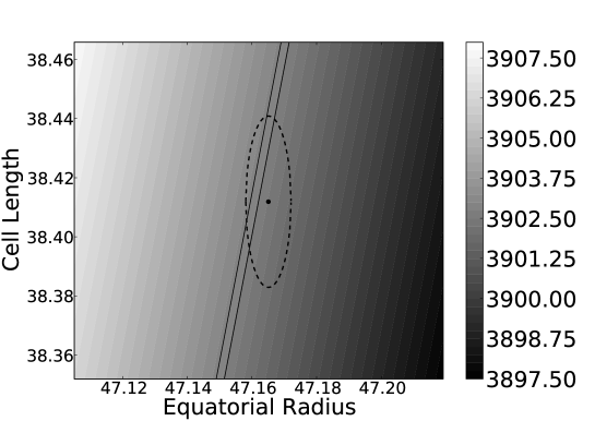
Figure 7: Plot of the dependency of frequency on the equatorial radius and the cell length produced by calculating frequency gradients dependent on varying both parameters and extracting frequencies. Also shown is the range of experimental values around the equatorial radius and cell length value, corresponding to $3902.810$ MHz with an experimental error of $\pm 95$ kHz, and the range of computed values given dimensional uncertainties.

VI Mode Extraction

As has been noted previously, an important property of this method is the ease with which modes can be extracted. To this end, we now consider the extraction of the five deflecting modes (i.e., the eigenvectors of the operator). Furthermore, for the $\pi$ deflection mode, we present a complete plot consisting of electric field lines, magnetic field lines, and the magnetic field magnitude on the cavity surface.

To begin, we revisit the algorithm for extracting modes and present the procedure with respect to the VORPAL software Nieter and Cary (2004), a finite-difference time-domain electromagnetic particle-in-cell code turned into an eigensolver for this work. VORPAL is a massively parallel code that stores data in the Hierarchical Data Format (HDF5) following the VizSchema viz conventions. This permits dumping of fields (magnetic or electric, for example) at arbitrary times for viewing with tools like VisIt vis .

Once the generalized eigenvalue problem $S^{\dagger}R\mathbf{a}_{m}=\lambda_{m}S^{\dagger}S\mathbf{a}_{m}$ is solved, the modes can be assembled according to

$${\bf v}_{m}=\sum_{\ell=1}^{L}a_{m,\ell}{\bf s}_{\ell}.$$ (15)

While ${\bf a}_{m}$ is the eigenvector of $S^{\dagger}R\mathbf{a}_{m}=\lambda_{m}S^{\dagger}S\mathbf{a}_{m}$, ${\bf v}_{m}$ is the eigenvector for the discrete operator $\nabla\times\nabla\times$. In a VORPAL simulation, the vectors ${\bf s}_{\ell}$ correspond to dumps of the magnetic (or electric) field at given times. A requirement is that all temporal dumps correspond entirely to the magnetic (or electric) field when constructing a magnetic (or electric) field mode.

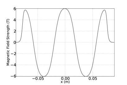
(a)  3902.810 MHz

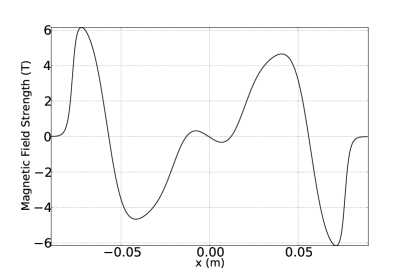
(b)  3910.404 MHz

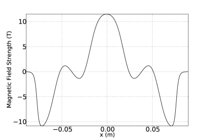
(c)  3939.336 MHz

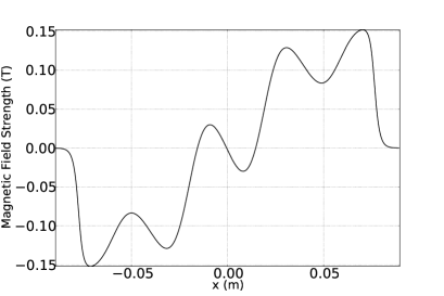
(d)  4001.342 MHz

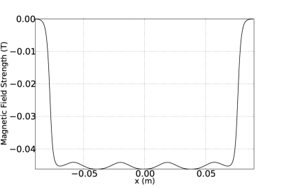
(e)  4106.164 MHz

Figure 8: Lineout of z-component of the magnetic field ($B_{z}$) at r=0 for the five deflecting (TM₁₁₀) modes of the A15 cavity. Simulations were ran at a resolution of $1.07\times 1.3\times 1.3\;\mathrm{mm}^{3}$ resulting in approximatley 1.05 million grid points. Each mode reconstruction, which consisted of constructing an hdf5 file as a linear combination of 20 hdf5 files, took less than a minute to perform.

As each ${\bf s}_{\ell}$ is represented by an HDF5 file, we must take linear combinations of multiple HDF5 files to assemble the modes. Python and its PyTables package are used to perform the assembly on a single processor. For approximately 1.05 million grid points it took less than a minute to perform a single mode assembly. In Fig. 8 we see the magnetic field of the five deflecting modes on a grid with a resolution of $1.07\times 1.3\times 1.3\;\mathrm{mm}^{3}$. The $\pi$ mode exhibits expected behavior. We also see the behavior exhibited by remaining deflecting modes.

In Fig. 9 we have assembled both the electric field and the magnetic field and also used a Python script to obtain the magnetic field magnitude on the cavity surface for the $\pi$ mode. The magnetic field magnitude shows areas on the cavity that may result in quenching, which is critical information that can be used by engineers and physicists considering cavity design.

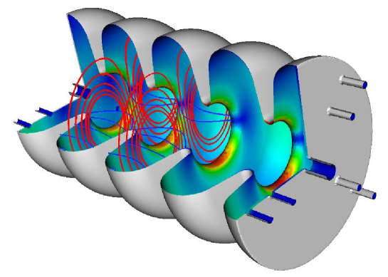
Figure 9: (Color online) Full representation of $\pi$ mode for the A15 cavity illustrating the electric (blue/darker) and the magnetic (red/lighter) field lines and the magnitude of the magnetic field painted on the inside of the cavity. All modes were constructed from simulations with post-processing to permit representation within the cavity. Image used with permission of the DOE SciDAC Office.

VII Conclusion

The frequency and mode extraction algorithm proposed in Ref. Werner and Cary (2008) in combination with the VORPAL computational framework Nieter and Cary (2004) has been shown to efficiently produce frequencies and modes for a realistic accelerator cavity, in this case a stack of four unpolarized dumbbells assembled in the form of a cavity that was designed in the past for an experimental program at Fermilab. We also showed that this method can extract the modes of the cavity. We estimated that this method, along with Richardson extrapolation, was able to compute frequencies to better than a part in $10^{5}$.

We further outlined the validation steps needed for determining whether this method is accurate. Given that the computational software had been verified, we proceeded through the validation process of considering errors in the measurement, failure to include relevant physics, and differences between the experiemental and computational geometrical models. Ultimately, we found that the computational frequency and the experimentally measured frequency were consistent to within the uncertainties (roughly $1\times 10^{-4}$), with the largest contributor to uncertainty resulting from imprecisely knowing the dimensions (particularly the equatorial radius) of the cavity. This is important, as it provides some guidance for future comparisons of calculations with measurements – namely, one must understand the dimensional uncertainties as a first step.

VIII Acknowledgments

This work was supported by the U.S. Department of Energy grants DE-FG02-04ER41317, DE-FC02-07ER41499, and DE-AC02-07CH11359.

We also thank the VORPAL team, T. Austin, G. I. Bell, D. L. Bruhwiler, R. S. Busby, M. Carey, J. Carlsson, J. R. Cary, Y. Choi, B. M. Cowan, D. A. Dimitrov, A. Hakim, J. Loverich, S. Mahalingam, P. Messmer, P. J. Mullowney, C. Nieter, K. Paul, C. Roark, S. W. Sides, N. D. Sizemore, D. N. Smithe, P. H. Stoltz, S. A. Veitzer, D. J. Wade-Stein, G. R. Werner, M. Wrobel, N. Xiang, C. D. Zhou.

References

- Werner and Cary (2008) G. Werner and J. Cary, J. Comput. Phys. 227, 5200 (2008).
- Nieter and Cary (2004) C. Nieter and J. Cary, J. Comput. Phys. 196, 448 (2004).
- M. Clemens et al. (1999) M. Clemens et al., in Proceedings of the 1999 Int. Conf. on Comp. Electromagnetics and its applications (1999), pp. 565–568.
- (4) M. McAshan and R. Wanzenberg, Fermi National Accelerator Lab Technical Note TM-2144.
- (5) L. Bellantoni, unpublished note.
- Neuhauser (1990) D. Neuhauser, J. Chem. Phys. 93, 2611 (1990).
- Neuhauser (1994) D. Neuhauser, J. Chem. Phys. 100, 5076 (1994).
- Wall and Neuhauser (1995) M. Wall and D. Neuhauser, J. Chem. Phys. 102, 8011 (1995).
- Mandelshtam and Taylor (1997) V. Mandelshtam and H. Taylor, J. Chem. Phys. 107, 6756 (1997).
- Mandelshtam (2003) V. Mandelshtam, J. Theor. Comput. Chem. 2, 497 (2003).
- Yee (1966) K. S. Yee, IEEE Trans. Antennas Propag. 14, 302 (1966).
- Bellantoni et al. (2001) L. Bellantoni, H. Edwards, M. McAshan, and R. Wanzenberg, in Conference: Particle Accelerator Conference, Chicago, IL (US), 06/18/2001–06/22/2001 (2001).
- Dey and Mittra (1997) S. Dey and R. Mittra, IEEE Microwave and Guided Wave Letters 7, 273 (1997).
- Nieter et al. (2009) C. Nieter, J. Cary, G. Werner, D. Smithe, and P. Stoltz, J. Comput. Phys. in review (2009).
- Burt et al. (2007) G. Burt, L. Bellantoni, and A. Dexter, EUROTeV-Report-2007-003 (2007).
- (16) VizSchema, https://ice.txcorp.com/trac/vizschema, last accessed July 8, 2009.
- (17) VisIt, http://visit.llnl.gov, last accessed July 8, 2009.