Formula for the Absorption Coefficient for Multi-Wall Nanotubes

Abstract

We present a formalism for calculating the absorption coefficient of a pair of coaxial tubules. A spatially nonlocal, dynamical self-consistent field theory is obtained by calculating the electrostatic potential produced by the charge density fluctuations as well as the external electric field. There are peaks in the absorption spectrum arising from plasma excitations corresponding either to plasmon or particle-hole modes. In this paper, we numerically calculate the plasmon contribution to the absorption spectrum when an external electric field is applied. The number of peaks depends on the radius of the inner as well as outer tubule. The height of each peak is determined by the plasmon wavelength and energy. For a chosen wave number, the most energetic plasmon has the highest peak corresponding to the largest oscillator strength of the excited modes. Some of the low-frequency plasmon modes have such weak coupling to an external electric field that they are not seen on the same scale as the modes with larger energy of excitation. We plot the peak positions of the plasmon excitations for a pair of coaxial tubules. The coupled modes on the two tubules are split by the Coulomb interaction. The energies of the two highest plasmon branches increase with the radius of the outer tubule. On the contrary, the lowest modes decrease in energy as this radius is increased. No effects due to inter-tubule hopping are included in these calculations.

I Introduction

Recently, there has been a considerable amount of effort to understand the spectroscopic properties of carbon nanotubes.new1a ; new1 ; new2 ; new3 ; new4 ; new5 ; new6 ; new7 In spectroscopic experiments, an external probe consisting of a beam of, for example, photons or electrons, perturbs the structure. Consequently, the ensuing charge density perturbation may be sustained by either single-particle excitations or collective plasmon modes. The density response may thus be measured through electron energy loss, photoemission, or absorption experiments, for example. So far, both theorists and experimentalists have investigated the plasma excitations of nanotubes using electron energy loss spectroscopy (EELS).new8 ; new9 ; new10 ; new11 ; new12 ; new13 ; new14 ; new15 ; new16 The theoretical formulation of EELS for nanotubes is now well established and several predictions concerning plasmon instabilities for nanotubes have been put forward.new8 In this paper, we present a theory for the absorption coefficient for a pair of coaxial tubules. The procedure can be generalized to multi-wall nanotubes. Several authorsnew1 ; new2 ; new3 have reported results for the optical absorption spectra of single-wall carbon nanotubes. The role played by the Coulomb interaction enters through the dielectric function. This was obtained for single-wall nanotubes using the random-phase approximation (RPA) as well as time-dependent density functional theory.new2 ; new3 ; new4 We separate the contributions to the absorption coefficient due to plasmon and single-particle excitations by carefully examining the dielectric function.

Our formalism relies on the use of the nonlocal dynamical response function. The reason is that this quantity determines the normal modes of oscillation which are identified as resonances. It is also responsible for the dielectric screening. We are able to separate the contributions from single-particle and plasmon excitations.new17 For simplicity, we use a continuum model to formulate our theory for the absorption coefficient. However, the formula which we develop may be adapted to nanotubes with bandstructures obtained using a basis set of localized orbitals.new4 We employ our results for the single-particle eigenstates to determine the frequency-dependent nonlocal dielectric function. We neglect disorder by assuming that we are dealing with high-quality nanotubes. For single-wall carbon nanotubes, the mean-free paths typically exceed 1$\mu$m. We use Maxwell’s equations for the electrostatic potential to calculate the dielectric response function of an electron gas on a nanotube in the RPA.new6 Our analysis is specific to a double-wall nanotube but it can be extended in a straightforward way to a multi-wall nanotubes.new7

Zhang, et al. chao calculated the dielectric response function for single-wall carbon nanotubes. These authors included the effect due to weak impurity scattering. Using their dielectric response function and our formula derived below, we would be able to identify the plasmon and single-particle excitations for multi-wall nanotubes with both electron-electron and electron-impurity scattering. Recently, the effects due to inter-tubule atomic hoppings and inter-tubule electron-electron interactions were included in calculations of the low-frequency electronic excitations of double-wall armchair carbon nanotubes.PLA It was demonstrated in Ref. PLA that the inter-tubule hopping significantly modifies the low-frequency plasmon excitations. For example, there are additional single-particle excitation channels and tunneling plasmon modes. We do include these effects arising from tunneling. However, within the framework of our calculations, these effects can be taken into account through the electron energy bandstructure.

The rest of this paper is organized as follows. In Sec. II, we use a self-consistent field theory involving Poisson’s equation and linear response of the charge density fluctuations to determine the induced potential. This potential is employed in the absorption coefficient whose resonances are determined by the plasma dispersion formula. We must separate the contributions from the single-particle and plasmon excitations when calculating the absorption coefficient. Gaps in the absorption coefficient for single-particle excitations correspond to pockets in the dispersion relation where the plasmons are not Landau damped. Numerical results demonstrating these assertions are presented in Sec. III. Concluding remarks are given in Sec. IV.

II General Formulation of the Problem

We now present a calculation for the absorption coefficient when an incident beam of light of frequency $\omega$ interacts weakly with a pair of coaxial tubules. In this case, linear response theory is applicable for calculating the rate at which energy is absorbed by the quantum system. The formalism we present below may be generalized to multi-wall cylindrical nanotubes consisting of an arbitrary number of coaxial tubules and to an array of parallel nanotubes, embedded in a material with dielectric constant $\epsilon_{b}$. We use Fermi’s golden rule for the rate at which energy is absorbed and then apply the fluctuation-dissipation theorem to the density-density correlation function.callaway After some algebra, we find that the absorption coefficient is given in terms of the real ($\Re e$) and imaginary ($\Im m$) parts of the Lorentz ratio $\alpha_{\rm Lorentz}(\omega)$. This is defined as the ratio of the Fourier coefficient of the absorbed energy at frequency $\omega$ of a probing field to the square of its amplitude and we havehaug

$$\beta_{\mbox{abs}}(\omega)=\frac{\omega}{n(\omega)\varepsilon_{b}c}\left[1+\rho_{\mbox{ph}}(\omega)\right]\ \Im m\ \alpha_{\rm Lorentz}(\omega)\ ,$$ (1)

where $\rho_{\mbox{ph}}(\omega)=\left[\exp(\hbar\omega/k_{B}T)-1\right]^{-1}$ is the photon distribution function, the refractive index is

$$n(\omega)=\left\{\frac{1}{2}\left[\epsilon_{b}+\Re e\ \alpha_{\rm Lorentz}(\omega)+\sqrt{\left(\epsilon_{b}+\Re e\ \alpha_{\rm Lorentz}(\omega)\right)^{2}+\left(\Im m\ \alpha_{\rm Lorentz}(\omega)\right)^{2}}\right]\right\}^{1/2}\ ,$$ (2)

and

$$\alpha_{\rm Lorentz}(\omega)=e\int d{\bf r}\ \delta n({\bf r},\omega)\frac{\phi_{\mbox{ext}}\left({\bf r}\right)}{\left|\nabla\phi_{\mbox{ext}}\left({\bf r}\right)\right|^{2}}\ .$$ (3)

Here, $\phi_{\mbox{ext}}\left({\bf r}\right)$ is an arbitrary external potential. However, for a uniform electric field, we have $\phi_{\mbox{ext}}\left({\bf r}\right)=-{\bf r}\cdot{\bf E}^{\mbox{ext}}$ for an electric field in the direction with unit vector $\hat{{\bf e}}_{0}={\bf E}^{\mbox{ext}}/\left|{\bf E}^{\mbox{ext}}\right|$. Also, the electron density fluctuation $\delta n({\bf r},\omega)$ on the two tubules of inner radius $R_{1}$ and outer radius $R_{2}$ arises from both the external electric field as well as the electric field from the induced potential, i.e., in linear response theory within the RPA, we have

$$\delta n({\bf r},\omega)\ =-e\int d{\bf r}^{\prime}\ \sum_{j=1}^{2}\chi_{j}^{0}\left({\bf r},{\bf r}^{\prime};\omega\right)\Phi_{\mbox{tot}}\left({\bf r}^{\prime},\omega\right)\ ,$$ (4)

where $\Phi_{\mbox{tot}}\left({\bf r},\omega\right)=\phi_{\mbox{ext}}\left({\bf r}\right)+\phi_{\mbox{ind}}\left({\bf r},\omega\right)$ is the sum of the external potential and the induced potential $\phi_{\mbox{ind}}\left({\bf r},\omega\right).$ The response function for the j^th tubule is given by

$$\chi_{j}^{0}\left({\bf r},{\bf r}^{\prime};\omega\right) = 2\sum_{\nu,\nu^{\prime}}\frac{f_{0}(\epsilon_{j,\nu^{\prime}})-f_{0}(\epsilon_{j,\nu})}{\hbar\omega+\epsilon_{j,\nu^{\prime}}-\epsilon_{j,\nu}}\Psi_{j,\nu}^{\ast}({\bf r}^{\prime})\Psi_{j,\nu^{\prime}}({\bf r}^{\prime})\Psi_{j,\nu^{\prime}}^{\ast}({\bf r})\Psi_{j,\nu}({\bf r})$$ (5)

$$\equiv \sum_{\nu,\nu^{\prime}}\Pi^{0}_{j,\nu\nu^{\prime}}(\omega)\Psi_{j,\nu}^{\ast}({\bf r}^{\prime})\Psi_{j,\nu^{\prime}}({\bf r}^{\prime})\Psi_{j,\nu^{\prime}}^{\ast}({\bf r})\Psi_{j,\nu}({\bf r})\ .$$

In this notation, $f_{0}(\epsilon)$ is the Fermi-Dirac distribution function, $\epsilon_{j,\nu}$ is an energy eigenvalue on the j^th tubule and $\Psi_{j,\nu}({\bf r})$ the corresponding eigenfunction. If an electron with effective mass $m^{\ast}$ is confined on the surface of a tubule of radius $R_{j}$, whose axis is taken to be on the $z$ axis, the eigenfunctions and eigenenergies are

$$\Psi_{j,\nu}(r,\varphi,z)=\frac{1}{\sqrt{L_{z}}}e^{ik_{z}z}\Phi_{j}(r)\frac{1}{\sqrt{2\pi R_{j}}}e^{il\varphi}\ ,\Phi_{j}^{2}(r)=\delta(r-R_{j})\ ,$$ (6)

$$\epsilon_{j,\nu}=\frac{\hbar^{2}k_{z}^{2}}{2m^{\ast}}+\frac{\hbar^{2}l^{2}}{2m^{\ast}R_{j}^{2}}\ ,$$ (7)

with $\displaystyle{\nu=\{k_{z},l\},\ k_{z}=\frac{2\pi n}{L_{z}}}$, $n,l=0,\pm 1,\pm 2,\cdots$ and $L_{z}$ is a normalization length. Plasmon excitations can be obtained by calculating the density matrix from its equation of motion $\displaystyle{i\hbar\frac{\partial\hat{\rho}}{\partial t}=[H,\hat{\rho}]}$. For small perturbations, $\hat{\rho}=\hat{\rho}_{0}+\hat{\rho}_{1}$ and $H=H_{0}-e\phi$, where $\hat{\rho}_{0}$ is the equilibrium density matrix and $\hat{\rho}_{1}$ its perturbation, $H_{0}$ is the unperturbed Hamiltonian and $\phi(r,\varphi,z;t)$ is the fluctuation in the electric potential corresponding to $\hat{\rho}_{1}$.

After we substitute Eq. (5) into Eq. (4), we obtain the following result for Eq. (3), i.e.,

$$\alpha_{\rm Lorentz}(\omega)=-e^{2}\sum_{j,\nu,\nu^{\prime}}\Pi^{0}_{j,\nu\nu^{\prime}}(\omega)\left\{Q_{j,\nu\nu^{\prime}}+U_{j,\nu\nu^{\prime}}(\omega)\right\}\ M_{j,\nu^{\prime}\nu}\ ,$$ (8)

where

$$M_{j,\nu\nu^{\prime}}=\int d{\bf r}\ \frac{\phi_{\mbox{ext}}\left({\bf r}\right)}{\left|\nabla\phi_{\mbox{ext}}\left({\bf r}\right)\right|^{2}}\ \Psi_{j,\nu}^{\ast}({\bf r})\Psi_{j,\nu^{\prime}}({\bf r})\ ,$$ (9)

$$Q_{j,\nu\nu^{\prime}}=\int d{\bf r}\ \phi_{\mbox{ext}}\left({\bf r}\right)\ \Psi_{j,\nu}^{\ast}({\bf r})\Psi_{j,\nu^{\prime}}({\bf r})\$$ (10)

are transition matrix elements and we have also introduced

$$U_{j,\nu\nu^{\prime}}(\omega)=\int d{\bf r}\ \phi_{\mbox{ind}}({\bf r},\omega)\ \Psi_{j,\nu}^{\ast}({\bf r})\Psi_{j,\nu^{\prime}}({\bf r})\ .$$ (11)

In the presence of an external potential $\phi_{\mbox{ext}}$, the induced potential is a solution of Poisson’s equation

$${\bf\nabla}^{2}\phi_{\mbox{ind}}({\bf r},\omega)=\frac{4\pi e}{\epsilon_{s}}\left(\delta n_{\mbox{ind}}({\bf r},\omega)-e\int d{\bf r}^{\prime}\sum_{j=1}^{2}\ \chi_{j}^{0}({\bf r},{\bf r}^{\prime};\omega)\ \phi_{\mbox{ext}}({\bf r}^{\prime})\right)\ .$$ (12)

The electrostatic potential $\phi_{\mbox{ind}}(r,\varphi,z;\omega)$ can be Fourier transformed with respect to the variables $\varphi$ and $z$ to give

$$\phi_{\mbox{ind}}(r,\varphi,z;\omega)=\sum_{q_{z},L}\phi_{\rm L}(r,q_{z},\omega)e^{iq_{z}z}e^{iL\varphi}\ ,\ q_{z}=\frac{2n\pi}{L_{z}}\ ,\ \ n,L=0,\pm 1,\pm 2,\cdots\ ,$$ (13)

so that Poisson’s equation becomes

$$\frac{1}{r}\frac{\partial}{\partial r}\left(r\frac{\partial\phi_{\rm L}(r,q_{z},\omega)}{\partial r}\right)-\frac{L}{r^{2}}\phi_{\rm L}(r,q_{z},\omega)-q^{2}\phi_{\rm L}(r,q_{z},\omega)$$ (14)

$$= \sum_{j=1}^{2}\left(A_{\rm L}^{(j)}(q_{z},\omega)+B_{\rm L}^{(j)}(q_{z}\ ,\omega)\right)\delta(r-R_{j})\ .$$

Here,

$$A_{\rm L}^{(j)}(q_{z},\omega) = \frac{-2e}{\varepsilon_{s}R_{j}}\sum_{l=-\infty}^{\infty}\int_{-\infty}^{\infty}dk_{z}\ \langle j,k_{z}l|\hat{\rho}_{1}|j,k_{z}-q_{z},l-L\rangle$$ (15)

$$= \frac{2e^{2}}{\varepsilon_{s}R_{j}}\phi_{\rm L}(R_{j},q_{z},\omega)\chi_{\rm j,L}(q_{z},\omega)$$

and $\hat{\rho}_{1}$ denotes the perturbed density matrix to lowest order in the external perturbation. The polarization function of the electron gas on each nanotube is defined by

$$\chi_{\rm j,L}(q_{z},\omega) = 2\sum_{l,l^{\prime}=-\infty}^{\infty}\int_{-\infty}^{\infty}\frac{dk_{z}}{2\pi}\frac{f_{0}(\epsilon_{j,k_{z},l})-f_{0}(\epsilon_{j,k_{z}-q_{z},l-L})}{\hbar\omega+\epsilon_{j,k_{z}-q_{z},l-L}-\epsilon_{j,k_{z},l}}$$ (16)

$$= \sum_{l=-\infty}^{\infty}\int_{-\infty}^{\infty}\frac{dk_{z}}{2\pi}\Pi^{0}_{j}(k_{z},l;k_{z}-q_{z},l-L)\ .$$

Also, in Eq. (14), we have introduced the quantity $B_{\rm L}^{(j)}(q_{z},\omega)$ which depends on the external electric field as follows

$$B_{\rm L}^{(j)}(q_{z},\omega) = \frac{-2e}{\varepsilon_{s}R_{j}}\sum_{l=-\infty}^{\infty}\int_{-\infty}^{\infty}dk_{z}\ \Pi^{0}_{j}(k_{z},l;k_{z}-q_{z},l-L)$$ (17)

$$\times \int d{\bf r}\ \Psi_{j,k_{z},l}^{\ast}({\bf r})\Psi_{j,k_{z}-q_{z},l-L}\phi_{\mbox{ext}}({\bf r})\ .$$

We now write the solution of Poisson’s equation for $\phi_{L}(r,q_{z},\omega)$ in Eq. (14) as

$$\phi_{L}(r,q_{z},\omega)=\left\{\matrix{\overline{C}_{1}I_{L}(q_{z}r),&r<R_{1}\cr\overline{C}_{3}I_{L}(q_{z}r)+\overline{C}_{4}K_{L}(q_{z}r),&R_{1}\leq r\leq R_{2}\cr\overline{C}_{2}K_{L}(q_{z}r),&r>R_{2}\cr}\right.\ ,$$ (18)

where $I_{L}(x)$ and $K_{L}(x)$ are Bessel functions of imaginary argument and $\overline{C}_{1}$, $\overline{C}_{2}$, $\overline{C}_{3}$ and $\overline{C}_{4}$ are functions of $q_{z}$ and $\omega$ but are independent of the radial coordinate $r$. These coefficients are determined from the continuity of $\phi_{L}(r,q_{z};\omega)$ at $r=R_{1},R_{2}$ and the step-like change of $\displaystyle{\frac{\partial\phi_{L}}{\partial r}}$ at $r=R_{1},R_{2}$, obtained by integrating Eq. (14) across the surfaces of the tubules. These boundary conditions together yield

$$\left(\matrix{I_{L}(q_{z}R_{1})&0&-I_{L}(q_{z}R_{1})&-K_{L}(q_{z}R_{1})\cr 0&-K_{L}(q_{z}R_{2})&I_{L}(q_{z}R_{2})&K_{L}(q_{z}R_{2})\cr-I_{L}^{\prime}(q_{z}R_{1})&0&I_{L}^{\prime}(q_{z}R_{1})&K_{L}^{\prime}(q_{z}R_{1})\cr 0&K_{L}^{\prime}(q_{z}R_{2})&-I_{L}^{\prime}(q_{z}R_{2})&-K_{L}^{\prime}(q_{z}R_{2})\cr}\right)\left(\matrix{\overline{C}_{1}\cr\overline{C}_{2}\cr\overline{C}_{3}\cr\overline{C}_{4}\cr}\right)=\left(\matrix{0\cr 0\cr\frac{A_{L}^{(1)}(q_{z},\omega)+B_{L}^{(1)}(q_{z},\omega)}{q_{z}}\cr\frac{A_{L}^{(2)}(q_{z},\omega)+B_{L}^{(2)}(q_{z},\omega)}{q_{z}}\cr}\right)\ .$$ (19)

In this notation, the prime on $I_{L}(x)$ and $K_{L}(x)$ indicates that a derivative with respect to the argument must be taken. This set of simultaneous equations show that $\overline{C}_{1},\ \overline{C}_{2},\ \overline{C}_{3}$ and $\overline{C}_{4}$ are determined by the induced potential through $A_{L}^{(j)}(q_{z},\omega),\ B_{L}^{(j)}(q_{z},\omega)$ on the right-hand side. On the other hand, the induced potential is determined by $\overline{C}_{j}$ in Eq. (18). This self-consistent field theory allows us to obtain the following analytic results for the coefficients as

$$\overline{C}_{1}(q_{z},\omega)=-R_{1}K_{L}(q_{z}R_{1})$$ (20)

$$\times \left[A_{L}^{(1)}(q_{z},\omega)+B_{L}^{(1)}(q_{z},\omega)\right]-R_{2}K_{L}(q_{z}R_{2})\left[A_{L}^{(2)}(q_{z},\omega)+B_{L}^{(2)}(q_{z},\omega)\right]\ ,$$

$$\overline{C}_{2}(q_{z},\omega)=-R_{1}I_{L}(q_{z}R_{1})$$ (21)

$$\times \left[A_{L}^{(1)}(q_{z},\omega)+B_{L}^{(1)}(q_{z},\omega)\right]-R_{2}I_{L}(q_{z}R_{2})\left[A_{L}^{(2)}(q_{z},\omega)+B_{L}^{(2)}(q_{z},\omega)\right]\ .$$

$$\overline{C}_{3}(q_{z},\omega)=-R_{2}K_{L}(q_{z}R_{2})\left[A_{L}^{(2)}(q_{z},\omega)+B_{L}^{(2)}(q_{z},\omega)\right]\ .$$ (22)

$$\overline{C}_{4}(q_{z},\omega)=-R_{1}I_{L}(q_{z}R_{1})\left[A_{L}^{(1)}(q_{z},\omega)+B_{L}^{(1)}(q_{z},\omega)\right]\ .$$ (23)

Making use of these results in Eq. (18), we obtain $\phi_{L}(R_{1},q_{z},\omega)=\overline{C}_{1}I_{L}(q_{z}R_{1})$ and $\phi_{L}(R_{2},q_{z},\omega)=\overline{C}_{2}K_{L}(q_{z}R_{2})$ on the surfaces of the tubules. Combining these results for $\phi_{L}(R_{j},q_{z},\omega)$ on the surface of the tubule with Eq. (15) where $A_{\rm L}^{(j)}(q_{z},\omega)$ is given in terms of $\phi_{\rm L}(R_{j},q_{z},\omega)$, these self-consistent field results yield

$$A_{\rm L}^{(1)}(q_{z},\omega)+B_{\rm L}^{(1)}(q_{z},\omega)=$$

$$\frac{1}{{\cal D}_{\rm L}(R_{1},R_{2};q_{z},\omega)}\left\{\varepsilon_{\rm L}^{(2)}(q_{z},\omega)B_{\rm L}^{(1)}(q_{z},\omega)-\frac{R_{2}}{R_{1}}V_{12}(q_{z})\chi_{\rm 1,L}(q_{z},\omega)B_{\rm L}^{(2)}(q_{z},\omega)\right\}$$ (24)

$$A_{\rm L}^{(2)}(q_{z},\omega)+B_{\rm L}^{(2)}(q_{z},\omega)=$$

$$\frac{1}{{\cal D}_{\rm L}(R_{1},R_{2};q_{z},\omega)}\left\{\varepsilon_{\rm L}^{(1)}(q_{z},\omega)B_{\rm L}^{(2)}(q_{z},\omega)-\frac{R_{1}}{R_{2}}V_{12}(q_{z})\chi_{\rm 2,L}(q_{z},\omega)B_{\rm L}^{(1)}(q_{z},\omega)\right\}\ ,$$ (25)

where

$$\varepsilon_{\rm L}^{(j)}(q_{z},\omega) = 1+\frac{2e^{2}}{\varepsilon_{s}}I_{L}(qR_{j})K_{L}(qR_{j})\chi_{{\rm j,L}}(q_{z},\omega)\ ,$$

$$V_{12}(q_{z}) = \frac{2e^{2}}{\varepsilon_{s}}I_{L}(qR_{1})K_{L}(qR_{2})$$

$${\cal D}_{\rm L}(R_{1},R_{2};q_{z},\omega) = \varepsilon_{\rm L}^{(1)}(q_{z},\omega)\varepsilon_{\rm L}^{(2)}(q_{z},\omega)-V_{12}^{2}(q_{z})\chi_{{\rm 1,L}}(q_{z},\omega)\chi_{{\rm 2,L}}(q_{z},\omega)\ .$$ (26)

In the absence of an external perturbation, $B_{L}^{(j)}(q_{z},\omega)=0$ and the nontrivial solutions for $A_{L}^{(j)}(q_{z},\omega)$ in Eqs. (24) and (25) correspond to ${\cal D}_{\rm L}(R_{1},R_{2};q_{z},\omega)=0$

We may now express $M_{j,\nu\nu^{\prime}}$ in Eq. (9) and $U_{j,\nu\nu^{\prime}}(\omega)$ in Eq. (11) in terms of Fourier series expansions with respect to the variables $\varphi$ and $z$. This was done for the induced potential in Eq. (13). We then have

$$M_{j,\nu\nu^{\prime}} = -\int d{\bf r}\ X\left({\bf r}\right)\ \Psi_{j,\nu}^{\ast}({\bf r})\Psi_{j,\nu^{\prime}}({\bf r})\$$ (27)

$$= -\sum_{q_{z}}\sum_{L=0,\pm 1,\pm 2,\cdots}\int d{\bf r}\ e^{iq_{z}z}e^{iL\varphi}\ \tilde{X}_{L}(k_{z})\ \Psi_{j,\nu}^{\ast}({\bf r})\Psi_{j,\nu^{\prime}}({\bf r})\ ,$$

where $X\left({\bf r}\right)\equiv\phi_{\mbox{ext}}\left({\bf r}\right)/\left|\nabla\phi_{\mbox{ext}}\left({\bf r}\right)\right|^{2}.$ We also use similar Fourier expansions for $Q_{j,\nu\nu^{\prime}}$ and $U_{j,\nu\nu^{\prime}}$ in Eqs. (10) and (11), respectively. When the eigenfunctions are substituted into Eq. (27), then we find that the only non-zero matrix elements occur when $l^{\prime}=l+L$ and $k_{z}^{\prime}=k_{z}+q_{z}$.

We can separate the contributions to the absorption coefficient from plasmons and single-particle excitations. The normal modes of oscillation for each tubule when the coupling $V_{12}$ between them is neglected are obtained by solving $\varepsilon_{\rm L}^{(j)}(q_{z},\omega)=0$. Below, we derive explicit results for the induced potential for a single tubule of radius R.

For a single tubule of radius R, we write the Fourier component of the induced potential as

$$\phi_{\rm L}(r,q_{z},\omega)=\left\{\matrix{C_{1}I_{L}(q_{z}r),&r<R\cr C_{2}K_{L}(q_{z}r),&r>R\cr}\right.\ .$$ (28)

After applying the boundary conditions on the surface of the tubule to the continuity of the potential and the discontinuity of its derivative, as seen in (14), we obtain

$$C_{1}(q_{z},\omega) = -\left[A_{\rm L}(q_{z},\omega)+B_{\rm L}(q_{z},\omega)\right]RK_{L}(q_{z}R)$$

$$C_{2}(q_{z},\omega) = -\left[A_{\rm L}(q_{z},\omega)+B_{\rm L}(q_{z},\omega)\right]RI_{L}(q_{z}R)\ ,$$ (29)

where $A_{\rm L}$ and $B_{\rm L}$ are as defined above for a tubule of radius R. We now use the results in Eq. (29) to obtain the electrostatic potential $\phi_{\rm L}(R,q_{z},\omega)$ on the surface of the tubule. When the derived result is substituted into Eq. (15), we obtain

$$A_{\rm L}(q_{z},\omega)+B_{\rm L}(q_{z},\omega)=\frac{B_{\rm L}(q_{z},\omega)}{\varepsilon_{\rm L}(q_{z},\omega)}\ ,$$ (30)

which can now be employed to calculate $\phi_{\rm L}(r,q_{z},\omega)$ in all regions by making use of Eqs. (28) and (29). Here, $\varepsilon_{\rm L}(q_{z},\omega)$ is given by $\varepsilon_{\rm L}^{(j)}(q_{z},\omega)Eq.\ (\ref{gae24})$ for a tubule of radius $R_{j}=R$.

In the absence of an external electric field, we must set $\phi_{\mbox{ext}}({\bf r})$ in Eq. (17) equal to zero. This results in $B_{\rm L}=0$ so that Eq. (30) reduces to $\epsilon_{\rm L}(q_{z},\omega)A_{\rm L}(q_{z},\omega)=0$, where $\epsilon_{\rm L}(q_{z},\omega)=1+(e^{2}/\epsilon_{s})I_{L}(q_{z}R)K_{L}(q_{z}R)\chi_{\rm L}(q_{z},\omega)$ is the dielectric function for the nanotube. A nontrivial solution for $A_{\rm L}(q_{z},\omega)$ leads to the plasma dispersion equation $\epsilon_{\rm L}(q_{z},\omega)=0$ for the self-sustaining plasma oscillations. However, in the presence of an external electric field, the solution of Eq. (30) for $A_{\rm L}(q_{z},\omega)$ in terms of $B_{\rm L}(q_{z},\omega)$ leads to the coefficients $C_{1}$ and $C_{2}$ in Eq. (29) as $C_{1}=-RK_{L}(q_{z}R)B_{\rm L}(q_{z},\omega)/\epsilon_{\rm L}(q_{z},\omega)$ and $C_{2}=-RI_{L}(q_{z}R)B_{\rm L}(q_{z},\omega)/\epsilon_{\rm L}(q_{z},\omega)$. When these results are substituted into Eq. (28), we obtain a closed-form analytic result for $\phi_{\rm L}(r,q_{z},\omega)$ and consequently $\phi_{\mbox{ind}}(r,\varphi,z;\omega)$ in Eq. (13) by making use of the Fourier series expansion. We may now use these results to obtain $U_{\alpha\alpha^{\prime}}(\omega)$ in Eq. (11) which could be employed in the Lorentz ratio in Eq. (8) for calculating the absorption coefficient $\beta_{\mbox{abs}}(\omega)$ in Eq. (1).

We now turn to analyzing the contributions to $\alpha_{\rm Lorentz}(\omega)$ in Eq. (8). This means that we must examine when the factor $\Im m\ \chi^{0}_{j,L}(\omega)\phi_{L}(R_{j},q_{z},\omega)\neq 0$. Thus, we must determine $\Im m\ {\cal D}_{\rm L}(R_{1},R_{2};q_{z},\omega)^{-1}=-\frac{{\cal D}_{\rm I}}{{\cal D}_{\rm I}^{2}+{\cal D}_{\rm R}^{2}}$ where ${\cal D}_{\rm R}$ and ${\cal D}_{\rm I}$ are the real and imaginary parts of ${\cal D}_{\rm L}$. Therefore, the only non-zero contributions to $\beta_{\mbox{abs}}(\omega)$ arise when either ${\cal D}_{\rm I}$ is finite, i.e., from the single-particle excitations, or when both ${\cal D}_{\rm R}$ and ${\cal D}_{\rm I}$ vanish simultaneously. This latter contribution comes from the plasmon excitations which are not Landau damped by the particle-hole modes.

III Numerical Results

In Fig. 2, we plot the plasmon contribution to the absorption coefficient when $L=0$ and $q_{z}=0.15\ k_{F}$ as a function of the incident photon energy for inner radius $R_{1}=10.0$ Å and several values of the radius $R_{2}$ of the outer tubule for a pair of coaxial tubules. In Fig. 3, the peak positions of the two highest branches of plasmon excitation energies for a pair of coaxial tubules are plotted as a function of $R_{2}/R_{1}$ for fixed $R_{1}=10.0$ Å. The parameters used to do our numerical calculations were chosen as follows. The electron effective mass $m^{\ast}=0.25\ m_{e}$, where $m_{e}$ is the free electron mass, the Fermi energy $E_{F}=0.6$ eV and the background dielectric constant $\epsilon_{b}=2.4$.new6 Our calculations show that the number of peaks depends on the chosen wave vector $q$ as well as the ratio $R_{2}/R_{1}$. However, for the range $0\leq q/k_{F}\leq 0.2$, the two highest branches are excited. There are some small amplitude oscillations on the curve in Fig. 3 representing the highest plasmon excitation energy. This behavior is caused by the variation in the number of occupied energy levels on the outer cylinder as $R_{2}$ is changed for a fixed number of electrons, i.e., $E_{F}$. The oscillations of the second highest branch are negligible because the pocket in the single-particle excitation spectrum where that branch exists is very narrow. The intensity (oscillator strength) of each peak is determined by the plasmon excitation energy. Consistently, the highest peak has the largest oscillator strength.new6 Some of the less energetic plasmon modes have such weak coupling to an external electric field that they are not seen on the scale we used in Fig. 2.

In Fig. 4, we plot the particle-hole mode contribution to the absorption for a pair of coaxial tubules. The curve in Fig. 4 is discontinuous Since the imaginary part of ${\cal D}$ is zero in the pockets where the plasmon frequencies exist. The gaps on the $\omega$-axis correspond to the pockets in the excitation spectrum where the collective plasmon modes exist. The dispersion of plasmon and single-particle excitations is given in Ref. —citenew6. , this accounts for the gaps on the frequency axis of Fig. 4. We chose $q_{z}=0.15\ k_{F}$ and all other parameters for the electron effective mass, Fermi energy and background dielectric constant are the same as Fig. 2. Unlike the plasmon contribution in Fig. 2, the particle-hole modes contribute over a wider range of frequency. The plasmon excitations occur within pockets between the particle-hole modes where they are Landau damped.new6 In Fig.  5, we plot these particle-hole mode frequencies versus $q_{z}/k_{F}$ for the pair of coaxial tubules used in Fig. 4. Numerical results for plasma excitations between subbands for which $L=1,2,\cdots$ may also be obtained from our formula for the absorption coefficient.

IV Concluding Remarks and Summary

In this paper, we gave a comprehensive formalism for calculating the absorption coefficient for a double-wall nanotube. The calculation was carried out using a self-consistent field approach for the induced potential and charge density fluctuations on the tubules. Our result is given in terms of the electron-electron interaction on each tubule and between the two tubules. We did not include any effects due to inter-tubule atomic hopping.PLA The effective dielectric function ${\cal D}_{\rm L}(R_{1},R_{2};q_{z},\omega)$ for the pair of tubules is expressed in terms of the dielectric functions $\varepsilon_{\rm L}^{(1)}(q_{z},\omega)$ and $\varepsilon_{\rm L}^{(2)}(q_{z},\omega)$ for each tubule, as shown in Eq. (26). The electron gas model for each tubule was used to simplify the calculations. However, a more realistic model whose energy bands are obtained using a tight-binding approximation for example, would be incorporated through the susceptibility $\chi_{{\rm 1,L}}(q_{z},\omega)$ and $\chi_{{\rm 2,L}}(q_{z},\omega)$ for each tubule. We showed that the loss function Im $\left[1/{\cal D}_{\rm L}(R_{1},R_{2};q_{z},\omega)\right]$ can be separated into contributions due to plasmon excitations and particle-hole modes. Figures 4 and 5 show that there are pockets within the particle-hole continuum where there is no Landau damping of the collective plasmon excitations. These regions could only be determined by separating the contributions to the loss function from the plasmon and single-particle excitations, as we described above. This separation would allow direct comparison between theory and experimental results of the absorption spectrum for plasma excitations on nanotubes.

Figure 1: Schematic of a pair of coaxial tubules.

Figure 2: The $L=0$ plasmon contribution to the absorption coefficient (arbitrary units) versus photon energy for $q_{z}=0.15\ k_{F}$, where $k_{F}=\sqrt{2m^{\ast}E_{F}/\hbar^{2}}$ with the radius of the inner tubule $R_{1}=10.0$ Å and several values of $R_{2}$. For clarity, the curves are shifted. From the bottom, the curves correspond to $R_{2}=20$ Å, 30 Å and 40 Å. The parameters used in the calculation are given in the text for $m^{\ast},\ E_{F}$ and $\epsilon_{b}$.

Figure 3: Peak positions for the $L=0$ and $q_{z}=0.15\ k_{F}$ plasmon excitations for the absorption coefficient for a pair of coaxial tubules as a function of $R_{2}/R_{1}$, for inner radius $R_{1}=10.0$ Å and outer radius $R_{2}$. The parameters used in the calculation are given in the text for $m^{\ast},\ E_{F}$ and $\epsilon_{b}$ and are the same as Fig. 2.

Figure 4: The $L=0$ particle-hole mode contribution to the absorption coefficient (arbitrary units) versus photon energy for $q_{z}=0.15\ k_{F}$, where $k_{F}=\sqrt{2m^{\ast}E_{F}/\hbar^{2}}$. The radius of the inner tubule $R_{1}=10.0$ Å and $R_{2}=20.0$ Å is the radius of the outer tubule . Only the frequency range where there are particle-hole modes contributes. The gaps on the frequency axis correspond to pockets where plasmon excitations are not Landau damped. The parameters used in the calculation are given in the text for $m^{\ast},\ E_{F}$ and $\epsilon_{b}$.

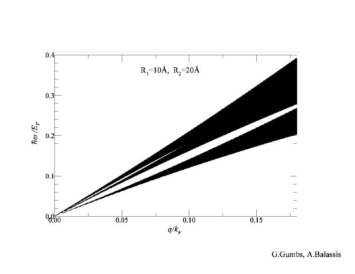
Figure 5: The dispersion relation for the $L=0$ continuum of particle-hole modes (shaded regions) for the pair of coaxial tubules used in Fig. 4.

References

• (1) G. Onida, L. Reining, and A. Rubio, Rev. Mod. Phys. 74, 601 (2002).
• (2) Z. M. Li, Z. K. Tang, H. J. Liu, N. Wang, C. T. Chan, R. Saito, S. Okada, G. D. Li, J. S. Chen, N. Nagasawa, and S. Tsuda, Phys. Rev. Lett. 87, 127401 (2001).
• (3) A. G. Marinopoulos, Lucia Reining, Angel Rubio, and Nathalie Vast, Phys. Rev. Lett. 91, 046402 (2003).
• (4) H. J. Liu and C. T. Chan, Phys. Rev. B66, 115416 (2002).
• (5) M. Machón, S. Reich, and C. Thomsen, D. Sánchez-Portal, and P. Ordej n, Phys. Rev. B66, 155410 (2002).
• (6) J. M. Pitarke and F. J. Garcia-Vidal, Phys. Rev. B63, 073404 (2001).
• (7) M. F. Lin and K. W.-K. Shung, Phys. Rev. B47, 6617 (1993); M. F. Lin and K. W. K. Shung, Phys. Rev. B50, 17 744 (1994); S. Tasaki, Koji Maekawa, and Tokio Yamabe, Phys. Rev. B57, 9301 (1998); M. F. Lin, F. L. Shyu, and R. B. Chen, Phys. Rev. B61, 14114 (2000); F. L. Shyu and M. F. Lin, Phys. Rev. B62, 8508 (2000).
• (8) Godfrey Gumbs and G. R. Aǐzin, Phys. Rev. B65, 195407 (2002).
• (9) A. Balassis and Godfrey Gumbs, Phys. Rev. B74, 045420 (2006).
• (10) Godfrey Gumbs and Antonios Balassis, Phys. Rev. B71, 235410 (2005).
• (11) C. W. Chiu, C. P. Chang, F. L. Shyu, R. B. Chen, and M. F. Lin, Phys. Rev. B67, 165421 (2003).
• (12) A. Rivacoba and F. J. Garc a de Abajo, Phys. Rev. B67, 085414 (2003).
• (13) Da-Peng Zhou, You-Nian Wang, Li Wei, and Z. L. Miskovic, Phys. Rev. A72, 023202 (2005).
• (14) N. R. Arista, Phys. Rev. A64, 032901 (2001).
• (15) N. R. Arista and M. A. Fuentes, Phys. Rev. B63, 165401 (2001).
• (16) N. R. Arista, Nucl. Instrum. Methods, Phys. Rev. B182, 109 (2001).
• (17) D. J. Mowbray, Z. L. Miskovic, F. O. Goodman, and You-Nian Wang, Phys. Rev. B70, 195418 (2004).
• (18) B. Zhao, I. Mönch, H. Vinzelberg, T. Mühl, and C. M. Schneider, Appl. Phys. Lett. 80, 3144 (2002).
• (19) C. Zhang, J. C. Cao, X. G. Guo, and Feng Liu, Appl. Phys. Lett. 90, 023106 (2007).
• (20) Y. H. Ho, G. W. Ho, S. C. Chen, J. H. Ho, and M. F. Lin, Phys. Rev. B76, 115422 (2007).
• (21) Joseph Callaway, Energy Band Theory (Academic Press, New York, 1964), p. 286.
• (22) Hartmut Haug and Stephan W. Koch, Quantum Theory of the Optical and Electronic properties of Semiconductors (World Scientific, Singapore, Third Edition, 2001), p. Chapter 1.
Refer to caption