Lyapunov Control on Quantum Open System in Decoherence-free Subspaces

Abstract

A scheme to drive and manipulate a finite-dimensional quantum system in the decoherence-free subspaces(DFS) by Lyapunov control is proposed. Control fields are established by Lyapunov function. This proposal can drive the open quantum system into the DFS and manipulate it to any desired eigenstate of the free Hamiltonian. An example which consists of a four-level system with three long-lived states driven by two lasers is presented to exemplify the scheme. We have performed numerical simulations for the dynamics of the four-level system, which show that the scheme works good.

I introduction

Manipulating the time evolution of a quantum system is a major task required for quantum information processing. Several strategies for the control of a quantum system have been proposed in the past decadedong09 , which can be divided into coherent and incoherent control, according to how the controls enter the dynamics. Among the quantum control strategies, Lyapunov control plays an important role in quantum control theory. Several papers have be published recently to discuss the application of Lyapunov control to quantum systemsvettori02 ; mirrahimi05 ; altafini07 ; yi09 . Although the basic mathematical formulism for Lyapunov control is well established, many questions remain when one considers its applications in quantum information processing, for instance, the Lyapunov control on open system and the state manipulation in its decoherence-free subspace.

As a collection of states that undergo unitary evolution in the presence of decoherence, the decoherence-free subspaces (DFS) zanardi97 and noiseless subsystem(NS)knill00 are promising concept in quantum information processing. Experimental realizations of DFS have been achieved with photons kwiat00 and in nuclear spin systems viola01 . A decoherence-free quantum memory for one qubit has been realized experimentally with two trapped ions kielpinski01 ; langer05 . An in-depth study of quantum stabilization problems for DFS and NS of Markovian quantum dynamics was presented inticozzi08 .

Most recently, we have proposed a scheme to drive an open quantum system into the decoherence-free subspacesyi09 . This scheme works also for closed quantum system, by replacing the DFS with a desired subspace. The result suggests that it is possible to drive a quantum system to a set of states (for example, the DFS in the paper), however it is difficult to manipulate the system into a definite quantum state in the DFS. The aim of this paper is to design a Lyapunov control to drive an open system to a definite state in the DFS. The Lyapunov control has been proven to be a sufficient simple control to be analyzed rigorously, in particular, the control can be shown to be highly effective for systems that satisfy certain sufficient conditions, which roughly speaking are equivalent to the controllability of the linearized system. In Lyapunov control, Lyapunov functions which were originally used in feedback control to analyze the stability of the control system, have formed the basis for new control design. By properly choosing the Lyapunov function, our analysis and numerical simulations show that the control scheme works good.

This paper is organized as follows. In Sec. II, we present a general analysis of Lyapunov control for open quantum systems, Lyapunov functions and control fields are given and discussed. To illustrate the general formulism, we exemplify a four-level system with 2-dimensional DFS in Sec. III, showing that the system can be controlled to a desired state in the DFS by Lyapunov control. Finally, we conclude our results in Sec. IV.

II general formulism

We can model a controlled quantum system either by a closed system, or by an open system governed by a master equation. In this paper, we restrict our discussion to a $N$-dimensional open quantum system, and consider its dynamics as Markovian and therefore the dynamics obeys the Markovian master equation ($\hbar=1,$ throughout this paper),

$$\dot{\rho}=-i[H,\rho]+{\mathcal{L}}(\rho),$$ (1)

where ${\mathcal{L}}(\rho)=\frac{1}{2}\sum_{m=1}^{M}\lambda_{m}([L_{m},\rho L_{m}^{\dagger}]+[L_{m}\rho,L_{m}^{\dagger}]),$ $H=H_{0}+\sum_{n=1}^{F}f_{n}(t)H_{n}$. $\lambda_{m}(m=1,2,...,M)$ are positive and time-independent parameters, which characterize the decoherence. $L_{m}(m=1,2,...,M)$ are jump operators. $H_{0}$ is a free Hamiltonian and $H_{n}(n=1,2,...,F)$ are control Hamiltonian, while $f_{n}(t)(n=1,2,...,F)$ are control fields. Equation (1) is of Lindblad form, this means that the solution to Eq. (1) has all the required properties of a physical density matrix at all times.

By definition, DFS is composed of states that undergo unitary evolution. Considering the fact that there are many ways for a quantum system to evolve unitarily, we focus on the DFS here that the dissipative part ${\mathcal{L}(\rho)}$ of the master equation is zero, leading to the following conditions for DFSkarasik08 . A space spanned by $\mathcal{H}_{DFS}=\{|\psi_{1}\rangle,|\psi_{2}\rangle,...,|\psi_{D}\rangle\}$ is a decoherence-free subspace for all time $t$ if and only if (1) $\mathcal{H}_{DFS}$ is invariant under $H_{0}$; (2) $L_{m}|\psi_{n}\rangle=c_{m}|\psi_{n}\rangle$ and (3) $\Gamma|\psi_{n}\rangle=g|\psi_{n}\rangle$ for all $n=1,2,...,D$ and $m=1,2,...,M$ with $g=\sum_{l=1}^{M}\lambda_{l}|c_{l}|^{2},$ and $\Gamma=\sum_{m=1}^{M}\lambda_{m}L_{m}^{\dagger}L_{m}.$ With these notations, the goal of this paper can be formulated as follows. We wish to apply a specified set of control fields $\{f_{i}(t),n=1,2,...,F\}$ in Eq. (1) such that $\rho(t)$ evolves into a desired state in the DFS and stays there forever. In contrast to the conventional control problemwangx09 , we here develop the control strategy to open system.

We use

$$V(\rho)=\text{Tr}(\rho\hat{A})$$ (2)

as a Lyapunov function, where $\hat{A}$ is hermitian and time-independent. First, we analyze the structure of critical points for $V(\rho)$ with restriction $\text{Tr}(\rho)=1.$ To determine the structure of $V(\rho)$ around one of its critical points, for example $\rho_{c}=\sum_{j}p_{j}^{c}|A_{j}\rangle\langle A_{j}|$ , we consider a finite variation $\delta\rho$ such that $\text{Tr}(\rho_{c}+\delta\rho)=1.$ Here we denote the normalized eigenvectors and eigenvalues of $\hat{A}$ by $|A_{i}\rangle$ and $A_{i}$ ($i=1,2,3,...,N$), respectively. Express $(\rho_{c}+\delta\rho)$ in the basis of the eigenvectors of $\hat{A},$

$$\rho_{c}+\delta\rho=\sum_{j}p_{j}^{c}|A_{j}+\delta A_{j}\rangle\langle A_{j}+\delta A_{j}|,$$

$$|A_{j}+\delta A_{j}\rangle=|A_{j}\rangle+\sum_{\alpha=1}^{N}\delta_{\alpha}^{j}|A_{\alpha}\rangle.$$ (3)

The normalization condition $\text{Tr}(\rho_{c}+\delta\rho)=1$ follows,

$$\sum_{j}p_{j}^{c}(\delta_{j}^{j*}+\delta_{j}^{j})+\sum_{j}p_{j}^{c}\sum_{\alpha}\delta^{j*}_{\alpha}\delta^{j}_{\alpha}=0.$$

Then

$$V(\rho_{c}+\delta\rho)-V(\rho_{c})=\sum_{j}p_{j}^{c}\sum_{\alpha\neq j}(A_{\alpha}-A_{j})\delta_{\alpha}^{j*}\delta_{\alpha}^{j}.$$ (4)

Considering $\delta_{\alpha}^{j}$ as variation parameters and noting $\delta_{\alpha}^{j*}\delta_{\alpha}^{j}\geq 0,$ we find that the structure of $V(\rho)$ around the critical point $\rho_{c}$ depends on the ordering of the eigenvalues: $\rho_{c}$ is a local maximum as a function of the variations $\delta_{\alpha}^{j}$ if and only if $A_{j}$ is the largest eigenvalue, a local minimum iff $A_{j}$ is the smallest eigenvalue and a saddle point otherwise. This observation leads us to suspect that the minimum of $V$ is asymptotically attractive, in other words, the control field based on this Lyapunov function would drive the open system to the eigenstate of $\hat{A}$ with the smallest eigenvalue. We will show through an example that this is exactly the case.

Now we establish the control fields $f_{n}(t).$ $V(\rho)=\text{Tr}(\rho\hat{A})$ yields,

$$\dot{V}=\text{Tr}({\mathcal{L}}(\rho)\hat{A})-i\text{Tr}(\rho[\hat{A},\sum_{n}f_{n}(t)H_{n}]),$$

where we choose $[\hat{A},H_{0}]=0,$ because ($\hat{a}$, $\hat{b}$ any operators) $\text{Tr}[\hat{a},\hat{b}]=0,$ i.e., the commutator can never be sign definite. The choice of $[\hat{A},H_{0}]=0$ implies that $H_{0}$ and $\hat{A}$ must have the same eigenvectors, then the control field would drive the open system into an eigenstate of the Hamiltonian $H_{0}$. To make $\dot{V}\leq 0,$ we choose a $f_{j_{0}}(t)$ such that

$$f_{j_{0}}(t)=-i\frac{\text{Tr}({\mathcal{L}}(\rho)\hat{A})}{\text{Tr}([\hat{A},H_{j_{0}}]\rho)},$$

$$f_{j}(t)=-i\kappa_{j}(\text{Tr}([\hat{A},H_{j}]\rho))^{*},\ \ \mbox{for}\ \ j\neq j_{0}.$$ (5)

Here $\kappa_{j}>0$ will be refereed as the strength of the control. Then the evolution of the open system with Lyapunov control can be described by the following nonlinear equations

$$\dot{\rho}(t) = -i[H_{0}+\sum_{n}f_{n}(t)H_{n},\rho(t)]+\mathcal{L}(\rho),$$ (6)

where $f_{n}(t)$ is determined by Eq.(5). It should be emphasized that $f_{j_{0}}$ always exists. To find $f_{j_{0}}$, $\text{Tr}([\hat{A},H_{j_{0}}]\rho)\neq 0$ is required. This can be done by construction. Now we show that $f_{j_{0}}$ is real. By the definition of $\mathcal{L}(\rho)$, $\mathcal{L}(\rho)$ is hermite, then $\text{Tr}({\mathcal{L}}(\rho)\hat{A})$ can be treated as the time derivative of $\langle\hat{A}\rangle$ and thus is real. Identifying $\hat{A}$ with a hermitian operator for a system described by the Hamiltonian $H_{j_{0}}$, we have $i\frac{\partial\hat{A}}{\partial t}=[\hat{A},H_{j_{0}}],$ so $\text{Tr}(i[\hat{A},H_{j_{0}}]\rho)$ is real. By the same virtue, we can show that all the control fields are real as long as the control Hamiltonian $H_{j}$ ($j=1,2,3...$) are hermitian.

By the LaSalle’s invariant principlelasalle61 , the autonomous dynamical system Eq.(6) converges to an invariant set defined by $\mathcal{E}=\{\dot{V}=0\}$. This set is in general not empty and of finite dimension, indicating that it is easy to manipulate an open system to a set of states but difficult to control it from an arbitrary initial state to a given target state. Fortunately, by elaborately designing the control Hamiltonian and the operator $\hat{A}$, we can solve this problem as follows. The invariant set defined by $\mathcal{E}=\{\dot{V}=0\}$ is an intersection of all sets $\mathcal{E}_{j}$ $(j=1,2,3,...)$, each one satisfies,

$$\text{Tr}(\hat{A}H_{j}\rho-H_{j}\hat{A}\rho)=0,$$

leading to $[\hat{A},\rho]=0$, $[\hat{A},H_{j}]=0$ or $[H_{j},\rho]=0$. By elaborately choosing $H_{j}$ ($j=1,2,3,...)$, we can set the contribution of $[\hat{A},H_{j}]=0$ and $[H_{j},\rho]=0$ to the intersection (i.e., the invariant set $\mathcal{E}$) to zero. In this case, the invariant set is a collection of state $\{\rho_{in}\}$ that satisfies $[\hat{A},\rho_{in}]=0.$ Considering that only the states in DFS are stable, we claim that we can manipulate the system from any initial state to the target state in DFS. In other words, we can design $\hat{A}$ such that $\mathcal{E}\bigcap\mbox{DFS}$ contains only the target state. We emphasis that although the control field $f_{j_{0}}(t)$ was specified to cancel $\text{Tr}(\mathcal{L}(\rho)\hat{A})$ in $\dot{V}$, it makes contribution to the dynamics of the open system.

III example

As an example of the Lyapunov control strategy, we discuss below a four-level system coupling to two external lasers, as shown in Fig. 1,

Figure 1: The schematic energy diagram. A four-level system with two degenerate stable states $|1\rangle$ and $|2\rangle$ in external laser fields. The two degenerate states are coupled to the excited state $|0\rangle$ by two separate lasers with coupling constants $\Omega_{1}$ and $\Omega_{2}$, respectively. While the stable state $|3\rangle$ is isolated from the other levels. The excited state $|0\rangle$ decays to $|j\rangle$ ($j=1,2,3$) with decay rate $\gamma_{j}$.

The Hamiltonian of such a system has the form

$$H_{0}=\sum_{j=0}^{2}\Delta_{j}|j\rangle\langle j|+(\sum_{j=1}^{2}\Omega_{j}|0\rangle\langle j|+h.c.),$$ (7)

where $\Omega_{j}\ \ (j=1,2)$ are coupling constants. Without loss of generality, in the following the coupling constants are parameterized as $\Omega_{1}=\Omega\cos\phi$ and $\Omega_{2}=\Omega\sin\phi$ with $\Omega=\sqrt{\Omega_{1}^{2}+\Omega_{2}^{2}}.$ The excited state $|0\rangle$ is not stable, it decays to the three stable states with rates $\gamma_{1}$, $\gamma_{2}$ and $\gamma_{3}$, respectively. We assume this process is Markovian and can be described by the Liouvillian,

$$\mathcal{L}(\rho)=\sum_{j=1}^{3}\gamma_{j}(\sigma_{j}^{-}\rho\sigma_{j}^{+}-\frac{1}{2}\sigma_{j}^{+}\sigma_{j}^{-}\rho-\frac{1}{2}\rho\sigma_{j}^{+}\sigma_{j}^{-})$$ (8)

with $\sigma_{j}^{-}=|0\rangle\langle j|$ and $\sigma_{j}^{+}=(\sigma_{j}^{-})^{\dagger}.$ It is not difficult to find that the two degenerate dark states

$$|D_{1}\rangle = \cos\phi|2\rangle-\sin\phi|1\rangle,$$

$$|D_{2}\rangle = |3\rangle,$$ (9)

of the free Hamiltonian $H_{0}$ form a DFS. Now we show how to control the system to a desired target state in the DFS. For this purpose, we choose the control Hamiltonian $H_{c}=\sum_{j=1}^{3}f_{j}(t)H_{j}$ with

$$H_{1}=\left(\begin{array}[]{cccc}1&1&1&1\\ 1&1&1&1\\ 1&1&1&1\\ 1&1&1&1\\ \end{array}\right),$$ (14)

$$H_{2}=|D_{1}\rangle\langle D_{2}|+|D_{2}\rangle\langle D_{1}|,$$

$$H_{3}=|0\rangle\langle D_{2}|+|D_{2}\rangle\langle 0|.$$ (15)

We shall use Eq. (5) to determine the control fields $\{f_{n}(t)\}$, and choose

$$|\Psi\rangle = \sin\beta_{1}\cos\beta_{3}|0\rangle+\cos\beta_{1}\cos\beta_{2}|1\rangle$$ (16)

$$+ \cos\beta_{1}\sin\beta_{2}|2\rangle+\sin\beta_{1}\sin\beta_{3}|3\rangle$$

as initial states for the numerical simulation, where $\beta_{1}$, $\beta_{2}$ and $\beta_{3}$ are allowed to change independently. We should emphasis that it is difficult to exhaust all possible initial states in the simulation, because for a 4-dimensional system, there are 15 independent real parameters needed to describe a general state, even for pure states, 6 real independent parameters are required. The initial state written in Eq.(16) omits all (three) relative phases between the states $|0\rangle,|1\rangle,|2\rangle$ and $|3\rangle$ in the superposition, and satisfies the normalization condition. $f_{1}(t)$ here is specified to cancel the contribution of $\text{Tr}[{\mathcal{L}}(\rho)\hat{A}]$ to $\dot{V},$ this means that $f_{1}(t)=-i\frac{\text{Tr}({\mathcal{L}}(\rho)\hat{A})}{\text{Tr}([\hat{A},H_{1}]\rho)},$ $f_{2}(t)$ and $f_{3}(t)$ are determined by Eq.(5).

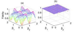
Figure 2: Fidelity of the system in the target state $|D_{1}\rangle$ (a), and in the DFS (b). The control field $f_{3}(t)$ is turned off, i.e., $f_{3}(t)=0.$ $\Omega=5,\phi=\frac{\pi}{5},\beta_{3}=\frac{\pi}{3},\gamma_{1}=\gamma_{2}=\gamma_{3}=\frac{1}{3}\gamma,\kappa_{2}=1,$ $\Delta_{0}=4,\Delta_{1}=\Delta_{2}=2$ and $\gamma=1.$

We have performed extensive numerical simulation with the initial states Eq.(16). Numerical results are presented in Figs. 2-4. The control field $f_{3}(t)$ plays an important role in this scheme as Fig. 2 shows. Fig. 2 tells us that without the control field $f_{3}(t)$, the open system can be driven into the DFS (with $\hat{A}$ given below), but it can not be manipulated into a definite state in DFS.

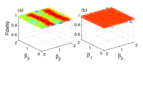
Figure 3: Fidelity of the control with $\hat{A}=|D_{2}\rangle\langle D_{2}|-|D_{1}\rangle\langle D_{1}|$ (i.e., the target state is $|D_{1}\rangle$) as a function of the initial states. The parameters chosen are the same as Fig. 2. The control strength $\kappa_{2}=1,\kappa_{3}=15$ were specified for this plot.

The physics behind is the following. With the given $\hat{A}$ (see below), $f_{1}(t)$ is always zero, so $H_{1}$ plays no role in the control. The only control that enters the system is $f_{2}(t)H_{2}$. From Eq.(5), we find that $f_{2}(t)$ takes zero provided $\rho=x|D_{2}\rangle\langle D_{2}|+(1-x)|D_{1}\rangle\langle D_{1}|,$ (where $x\geq 0)$, leading to the above observation. When the control field $f_{3}(t)$ is turned on. The four-level system can be controlled to a desired state in DFS by properly choosing $\hat{A}.$

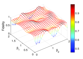
Figure 4: Fidelity of the control versus initial states. The target state is $|D_{2}\rangle$ (or $\hat{A}=-|D_{2}\rangle\langle D_{2}|+|D_{1}\rangle\langle D_{1}|$). $\kappa_{3}=15$, the other parameters chosen are the same as in Fig.2 are chosen for this plot.

For example, when $\hat{A}=\hat{A}_{1}=|D_{2}\rangle\langle D_{2}|-|D_{1}\rangle\langle D_{1}|,$ the system can be controlled into $|D_{1}\rangle$ (see Fig.3), whereas $\hat{A}=-\hat{A}_{1}$ can drive the system into $|D_{2}\rangle$ (see Fig.4). Based on the formalism in Sec. II, $\hat{A}=\hat{A}_{1}$ together with the controls could drive the system to the eigenstate of $\hat{A}_{1}$ with smallest eigenvalue (namely, $|D_{1}\rangle$), and to $|D_{2}\rangle$ with $\hat{A}=-\hat{A}_{1}.$ As figure 4 shows, however, the fidelity is not 1 for some initial states, for example $\beta_{1}=0.$ The reason is as follows. Though the choice of $\hat{A}=-\hat{A}_{1}$ benefits the target state $|D_{2}\rangle$, since $|D_{2}\rangle$ is the eigenstate of $\hat{A}$ with smallest eigenvalue, the control $H_{3}=(|0\rangle\langle D_{2}|+h.c.)$ does not favor the control target $|D_{2}\rangle$, because $H_{3}$ couples the states $|0\rangle$ and $|D_{2}\rangle$, and $|0\rangle$ decays to the three stable states equally. This observation suggests that $h_{3}=(|0\rangle\langle D_{1}|+h.c.)$ instead of $H_{3}$ could help the control when the target is $|D_{2}\rangle.$ Indeed further numerical simulations confirm this prediction that the control $h_{3}$ can drive the system into $|D_{2}\rangle$ with almost perfect fidelity $99\%$.

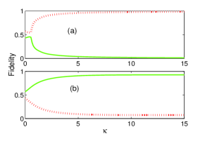
Figure 5: Fidelity as a function of the control strength $\kappa_{3}=\kappa$. (a)$\hat{A}=|D_{2}\rangle\langle D_{2}|-|D_{1}\rangle\langle D_{1}|,$ (b)$\hat{A}=-|D_{2}\rangle\langle D_{2}|+|D_{1}\rangle\langle D_{1}|.$ $\phi=\frac{\pi}{4},\beta_{1}=\frac{\pi}{6},\beta_{2}=\frac{\pi}{3},\beta_{3}=\frac{\pi}{5},$ and $\kappa_{2}=1.$ The other parameters chosen are the same as Fig. 2.

The fidelity of the open system in the target state depends on the strength $\kappa_{3}=\kappa$ of the control $f_{3}(t),$ the dependence is plotted in Fig.5. With large $\kappa$, the system would asymptotically converge to the target state as Fig.5 shows. As expected, the control fields $f_{2}(t)$ and $f_{3}(t)$ tend to zero when the open system converges to the target state, see Fig.6

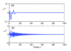
Figure 6: Control field $f_{2}(t)$ and $f_{3}(t)$ as a function of time. $\Omega=5,\phi=\frac{\pi}{5},\beta_{1}=\frac{\pi}{5},\beta_{2}=\frac{\pi}{4},\beta_{3}=\frac{\pi}{6},\kappa_{2}=1,$ and $\kappa_{3}=15.$ $\hat{A}=|D_{2}\rangle\langle D_{2}|-|D_{1}\rangle\langle D_{1}|.$ $f_{1}(t)$ is zero in this scheme.

IV conclusion

In summary, we have proposed a scheme to manipulate an open quantum system in the decoherence-free subspaces. This study was motivated by the fact that for Lyapunov control, it is usually difficult to optimally control the system from an arbitrary initial state to a given target state, this is due to the LaSalle’s invariant principle. Our present study suggests that it is possible to drive a quantum system to a desired state in DFS by elaborately designing the controls. The results do not break the LaSalle’s role, instead it reduces the invariant set $\mathcal{E}$ to include the target state only. To demonstrate the proposal we exemplify a four-level system and numerically simulate the controlled dynamics. The dependence of the fidelity on initial states as well as the control fields are calculated and discussed. This scheme put the Lyapunov control on quantum open system one step forward, and shed light on the quantum control in DFS.

This work is supported by NSF of China under grant Nos. 10775023 and 10935010.

References

- (1) Daoyi Dong, Ian R Petersen, Quantum control theory and applications: A survey, arXiv:0910.2350; C. Brif, R. Chakrabarti, H. Rabitz, Control of quantum phenomena: Past, present, and future, arXiv:0912.5121, and the references therein.
- (2) P. Vettori, in Proceedings of the MTNS Conferene, 2002; A. Ferrante, M. Pavon, and G. Raccanelli, in Proceedings of the 41st IEEE Conference on Decision and Control, 2002; S. Grivopoulos and B. Bamieh, in Proceedings of the 42nd IEEE Conference on Decision and Control, 2003; M. Mirrahimi and P. Rouchon, in Proceedings of IFAC Symposium LOLCOS 2004; In Proceedings of the International Symposium MTNS 2004.
- (3) M. Mirrahimi, P. Rouchon, and G. Turinici, Automatica 41, 1987(2005);
- (4) C. Altafini, Quantum Information Processing 6, 9(2007).
- (5) X. X. Yi, X. L. Huang, Chunfeng Wu, and C. H. Oh, Phys. Rev. A 80, 052316(2009).
- (6) P. Zanardi and M. Rasetti, Phys. Rev. Lett. 79, 3306 (1997); D. A. Lidar, I. L. Chuang, and K. B. Whaley, Phys. Rev. Lett. 81, 2594 (1998); J. Kempe, D. Bacon, D. A. Lidar, and K. B. Whaley, Phys. Rev. A 63, 042307 (2001); D. A. Lidar and K. B. Whaley, in Irreversible Quantum Dynamics, edited by F. Benatti and R. Floreanini, (Springer Lecture Notes in Physics vol. 622, Berlin, 2003), pp. 83-120; A. Shabani and D. A. Lidar, Phys. Rev. A 72, 042303 (2005).
- (7) E. Knill, R. Laflamme, and L. Viola, Phys. Rev. Lett. 84, 2525 (2000).
- (8) P. G. Kwiat, A. J. Berglund, J. B. Altepeter, and A. G. White, Science 290, 498 (2000); M. Mohseni, J. S. Lundeen, K. J. Resch, and A. M. Steinberg, Phys. Rev. Lett. 91, 187903 (2003); J. B. Altepeter, P. G. Hadley, S. M. Wendelken, A. J. Berglund, and P. G. Kwiat, Phys. Rev. Lett. 92, 147901 (2004); Q. Zhang, J. Yin, T.-Y. Chen, S. Lu, J. Zhang, X.-Q. Li, T. Yang, X.-B. Wang, and J.-W. Pan, Phys. Rev. A 73, 020301(R) (2006).
- (9) L. Viola, E. M. Fortunato, M. A. Pravia, E. Knill, R. Laflamme, and D. G. Cory, Science 293, 2059 (2001); J. E. Ollerenshaw, D. A. Lidar, and L. E. Kay, Phys. Rev. Lett. 91, 217904 (2003); D. Wei, J. Luo, X. Sun, X. Zeng, M. Zhan, and M. Liu, Phys. Rev. Lett. 95, 020501 (2005).
- (10) D. Kielpinski, V. Meyer, M. A. Rowe, C. A. Sackett, W. M. Itano, C. Monroe, and D. J. Wineland, Science 291, 1013 (2001).
- (11) C. Langer, R. Ozeri, J. D. Jost, J. Chiaverini, B. De- Marco, A. Ben-Kish, R. B. Blakestad, J. Britton, D. B. Hume, W. M. Itano, D. Leibfried, R. Reichle, T. Rosenband, T. Schaetz , P. O. Schmidt, and D. J. Wineland, Phys. Rev. Lett. 95, 060502 (2005).
- (12) F. Ticozzi, L. Viola, IEEE Trans. Aut. Control 53, 2048(2008);F. Ticozzi, L. Viola,Automatica 45, 2002(2009).
- (13) R. I. Karasik, K. P. Marzlin, B. C. Sanders, and K. B. Whaley, Phys. Rev. A 77, 052301(2008).
- (14) Xiaoting Wang and S. G. Schirmer, arXiv:0805.2882; 0901.4515; 0901.4522.
- (15) J. LaSalle and S. Lefschetz, Stability by Lyapunov’s Direct Method with Applications (Academic Press, New York, 1961).