Stochastic effects at ripple formation processes in anisotropic systems with multiplicative noise

Abstract

We study pattern formation processes in anisotropic system governed by the Kuramoto-Sivashinsky equation with multiplicative noise as a generalization of the Bradley-Harper model for ripple formation induced by ion bombardment. For both linear and nonlinear systems we study noise induced effects at ripple formation and discuss scaling behavior of the surface growth and roughness characteristics. It was found that the secondary parameters of the ion beam (beam profile and variations of an incidence angle) can crucially change the topology of patterns and the corresponding dynamics.

PACS 05.40.-a, 05.70.Ln, 64.60.l, 68.35.Ct, 79.20.Rf

1 Introduction

A fabrication of nanoscale surface structures have attracted a considerable attention due to their applications in electronics [1]. In the last five decades many studies have been devoted to understanding the mechanism of pattern formation and its control during ion-beam sputtering (see, for example Refs.[2, 3, 4, 5, 6, 7, 8, 9]). Among theoretical investigations there are a lot of experimental data manifesting a large class of patterns appeared as result of self-organization process on the surface of a solid. It was shown experimentally that main properties of pattern formation and structure of patterns depend on the energetic ion-beam parameters such as ion flux, energy of deposition, angle of incidence and temperature. Formation of ripples was investigated on different substrates, i.e. on metals ($Ag$ and $Cu$) [10, 11] on semiconductors ($Ge$ [12] and $Si$ [13, 14, 15]) on $Sn$ [16], $InP$ [17], on $Cd_{2}Nb_{2}O_{7}$ pyrochlore [18] and other. Height modulations on the surface induced by ion-beam sputtering result in formation of ripples having the typical size of 0.1 to 1 $\mu m$ and nanoscale patterns with the linear size of 35 to 250 $A$ [19].

It is well known that orientation of ripples depends on the incidence angle. At the incidence angles around $\pi/2$ the wave-vector of the modulations is parallel to the component of the ion beam in the surface plane, whereas at small incidence angles (close to grazing) the wave-vector is perpendicular to this component. The orientation of ripples can be controlled by a penetration depth which is proportional to the deposited energy. Analytical investigations provided by Cuerno and Barabasi show a possible control of pattern formation governed by both the incidence angle and penetration depth [4, 5]. The main theoretical models describing ripple formation are based on results of the famous works of Bradley and Harper [3], Kardar, Parisi, and Zhang [20], Wolf and Villian [21], Kuramoto and Sivashinsky [22]. The main mechanisms for pattern formation were set to predict orientation change of the ripples, formation of holes and dots. These models were generalized taking into account additive fluctuations leading to statistical description of the corresponding processes.

Moreover, it was shown that under well defined processing conditions the secondary ion-beam parameters (beam profile) may lead to different patterns [23]. Theoretical predictions including statistical properties of the beam profile were performed in Ref.[9]. It was shown that fluctuations in incident angles result in stochastic description of the ripple formation with multiplicative noise. Unfortunately, detailed description of pattern formation in such complicated stochastic systems was not discussed. Moreover, the problem of understanding the scaling behavior of the surface characteristics is still opened.

In this article we aim to study ripple (or generally pattern) formation processes in anisotropic system governed by the corresponding Kuramoto-Sivashinsky equation which takes into account multiplicative noise caused by fluctuation of the incidence angle. We consider the linear and nonlinear models separately and discuss the corresponding phase diagrams in the space of main beam parameters reduced to the penetration depth and the incidence angle. Moreover, we present results of the scaling behavior study of the correlation functions and discuss time dependencies of the roughness and growth exponents during the system evolution as well as fractal properties of the surface. It will be shown that multiplicative fluctuations in ripple formation processes can accelerate/delay surface modulations. We shall show that both phase diagrams and the scaling exponents crucially depend on the statistical properties of the beam.

The work is organized as follows. In Section 2 we present the stochastic model with multiplicative noise. Section 3 is devoted to the stability analysis of the linear system, where the main phase diagrams are discussed. The nonlinear stochastic model is studied in Section 4. Here we consider the behavior of the main statistical characteristics of the surface such as distribution of the height field, scaling properties of the correlation functions. We summarize in Section 5.

2 Model

Let us consider a $d$-dimensional substrate and denote with $\mathbf{r}$ the $d$-dimensional vector locating a point on it. The surface is described at each time $t$ by the height $z=h(\mathbf{r},t)$. If we assume that the surface morphology is changed while ion sputtering, then we can use the model for the surface growth proposed by Bradley and Harper [3] and further developed by Cuerno and Barabasi [4]. We consider the system where the direction of the ion beam lies in $x-z$ plane at an angle $\theta$ from the normal of the uneroded surface. Following the standard approach one assumes that an averaged energy deposited at the surface (let say point $O$) due to the ion arriving at the point $P$ in the solid follows the Gaussian distribution [3] $E(\mathbf{r})=(\epsilon/(2\pi)^{3/2}\sigma\mu^{2})\exp(-z^{2}/2\sigma^{2}-(x^{2}+y^{2})/2\mu^{2})$; $\epsilon$ denotes the kinetic energy of the arriving ion, $\sigma$ and $\mu$ are the widths of the distribution in directions parallel and perpendicular to the incoming beam. Parameters $\sigma$ and $\mu$ depend on the target material and can vary with physical properties of the target and incident energy. We consider the simplest case when $\sigma=\mu$. The erosion velocity at the surface point $O$ is described by the formula $v=p\int_{\mathcal{R}}{\rm d}\mathbf{r}\Phi(\mathbf{r})E(\mathbf{r})$, where integration is provided over the range of the energy distribution of all ions; here $\Phi(\mathbf{r})$ and $p$ are corrections for the local slope dependence of the uniform flux $J$ and proportionality constant, respectively [24]. The general expression for the local flux for surfaces with non-zero local curvature is [25]: $\Phi(x,y,h)=J\cos\left(\arctan\left[\sqrt{(\nabla_{x}h)^{2}+(\nabla_{y}h)^{2}}\right]\right)$. Hence, the dynamics of the surface height is defined by the relation $\partial_{t}h\simeq-v(\theta-\nabla_{x}h,\nabla_{x}^{2}h,\nabla_{y}^{2}h)$ and is given by the equation $\partial_{t}h\simeq-v(\theta)\sqrt{1+(\nabla h)^{2}}$, where $0<\theta<\pi/2$ [3, 27, 4, 20, 5]. The linear term expansion gives $\partial_{t}h=-v_{0}+\gamma\nabla_{x}h+\nu_{\alpha}\nabla_{\alpha\alpha}^{2}h$; where $\nabla=\partial/\partial\mathbf{r}$, $\nabla_{\alpha}=\partial/\partial\alpha$, $\alpha=\{x,y\}$. Here $v_{0}$ is the surface erosion velocity; $\gamma=\gamma(\theta)$ is a constant that describes the slope depending erosion; $\nu_{\alpha}=\nu_{\alpha}(\theta)$ is effective surface tension generated by erosion process in $\alpha$ direction.

If one assumes that the surface current is driven by differences in chemical potential $\mu$, then the evolution equation for the field $h$ should take into account the term $-\nabla\cdot\mathbf{j}_{s}$ in the right hand side, where $\mathbf{j}_{s}=K\nabla(\nabla^{2}h)$ is the surface current; $K>0$ is the temperature dependent surface diffusion constant. If the surface diffusion is thermally activated, then we have $K=D_{s}\kappa\rho/n^{2}T$, where $D_{s}=D_{0}e^{-E_{a}/T}$ is the surface self-diffusivity ($E_{a}$ is the activation energy for surface diffusion), $\kappa$ is the surface free energy, $\rho$ is the areal density of diffusing atoms, $n$ is the number of atoms per unit volume in the amorphous solid. This term in the dynamical equation for $h$ is relevant in high temperature limit which will be studied below.

Quantities $v_{0}$, $\gamma$, $\nu_{\alpha}$ are functions of the angle $\theta$ only, not the temperature. Assuming that the surface varies smoothly, next we neglect spatial derivatives of the height $h$ of third and higher orders in the slope expansion. Taking into account nonlinear terms in the slope expansion of the surface height dynamics, we arrive at the equation for the quantity $h^{\prime}=h+v_{0}t$ of the form [3, 4]

$$\partial_{t}h=\gamma\nabla_{x}h+\nu_{\alpha}\nabla_{\alpha\alpha}^{2}h+\frac{\lambda_{\alpha}}{2}(\nabla_{\alpha}h)^{2}-K\nabla^{2}(\nabla^{2}h),$$ (1)

where we drop the prime for convenience. Coefficients in Eq.(1) are defined in Ref.[4] and read

$$s=\sin\theta,\quad c=\cos\theta,\quad a_{\sigma}=a/\sigma,\quad F\equiv(\epsilon pJ/\sqrt{2\pi})\exp(-a_{\sigma}^{2}/2),$$

$$\gamma=\frac{F}{\sigma}s(a_{\sigma}^{2}c^{2}-1),$$

$$\lambda_{x}=\frac{F}{\sigma}c(a_{\sigma}^{2}(3s^{2}-c^{2})-a_{\sigma}^{4}s^{2}c^{2}),\quad\lambda_{y}=-\frac{F}{\sigma}c(a_{\sigma}^{2}c^{2}),$$

$$\nu_{x}=\frac{F}{2}a_{\sigma}(2s^{2}-c^{2}-a_{\sigma}^{2}s^{2}c^{2}),\quad\nu_{y}=-\frac{F}{2}a_{\sigma}c^{2}$$

Here all control parameters are defined through the ion penetrate distance $a$, the incidence angle $\theta$, the flux $J$ and the kinetic energy $\epsilon$. It is known [25] that the penetration depth depends on the target material properties and the incoming ion energy $\epsilon$: $a\approx\epsilon^{2m}/nC_{m}$, where $n$ is the target atom density, $C_{m}$ is the constant depending on the interatomic interaction potential [26], $m\approx 1/2$ for intermediate energies (from 1 to 100 keV). Equation (1)is known as the noiseless anisotropic Kuramoto-Sivashinsky equation [22]

It was shown [3] that the linearized dynamical equation (1) admits a solution of the form $h(x,y,t)=A\exp(i(k_{x}x+k_{y}y-\omega t)-rt)$, where $\omega=-\gamma(\theta)k_{x}$ is the frequency, $r=-(\nu_{x}(\theta)k_{x}^{2}+\nu_{y}(\theta)k_{y}^{2})-K(k_{x}^{2}+k_{y}^{2})^{2}$ is the parameter responsible for a stability of the solution. During the system evolution a selection of wave-numbers responsible for ripple orientation occurs. The selected wave-number is $k^{2}_{\alpha}=|\nu_{\alpha}|/2K$, where $\alpha$ refers to the direction ($x$ or $y$) along which the associated $\nu_{\alpha}$ has smaller value.

For the noiseless nonlinear model (1) it was shown that due to the sets $\nu_{\alpha}$ and $\lambda_{\alpha}$ are the functions of the incidence angle $\theta\in[0,\pi/2]$ there are three domains in the phase diagram $(a_{\sigma},\theta)$ where $\nu_{x}$ and $\lambda_{x}$ changes their signs, separately [4]. It results in ripples formation in different direction $x$ or $y$ varying $a_{\sigma}$ or $\theta$.

To describe an evolution of the surface in more realistic conditions one should take into account that the bombarding ions reach the surface stochastically, i.e. at random position and time; generally, it can reach the surface at random angle lying in the vicinity of the incidence angle $\theta$. Most of models proposed to describe ripple formation due to the ion sputtering process incorporates additive fluctuations $\xi(\mathbf{r},t)$ that takes into account stochastic nature of arriving ions (see for example Refs.[4, 6, 14]). From the mathematical viewpoint such stochastic source results in spreading the patterns and makes possible statistical description of the system. If this term is assumed as a Gausisan white noise in time and space it can not change the system behavior crucially [28, 29].

If one supposes that the ion beam is composed of ions distributed with different incidence angles, then we have three possible cases [9]: (i) homogeneous beam when the erosion velocity depends upon random ion beam parameters and the average velocity is defined through the distribution function over beam directions; (ii) temporally fluctuating homogenous beam when the direction of illumination constitutes a stationary, temporally homogeneous stochastic process; (iii) spatio-temporally fluctuating beam when the directions of ions form a homogeneous and stationary field. In Ref.[9] authors consider the case (iii) under assumption of the Gaussian distribution of a beam profile centered at a fixed angle $\theta_{0}$. Such model means that the fluctuation term that can appear in the dynamical equation for the field $h$ is some kind of a multiplicative noise (with intensity depending on the field $h$). Unfortunately only general perspectives were reported for the nonlinear model, whilst main results relate to studying the linear model behavior. From the naive consideration one can expect that the multiplicative noise can qualitatively influence on the dynamics of ripple formation in the nonlinear system.

In present article we aim to consider the general problem of the ripple formation under assumption of Gaussian distribution of the beam profile around $\theta_{0}$ in the framework of the model given by Eq.(1) following the approach proposed in Ref.[9]. To describe the model we start from Eq.(1) which can be rewritten in the form $\partial_{t}h=f(\theta,\nabla_{\alpha}h)$, where $f$ is a deterministic force. Considering small deviations from the fixed angle $\theta_{0}$ we can expand the function $f(\theta,\nabla_{\alpha}h)$ in the vicinity of $\theta_{0}$. Therefore, for the right hand side we get $f=f_{0}+(\partial f/\partial\theta)|_{\theta=\theta_{0}}\delta\theta$ and assume that $\delta\theta$ is a stochastic field, i.e. $\delta\theta=\delta\theta(\mathbf{r},t)$. Assuming Gaussian properties for the stochastic component $\delta\theta$, we set

$$\langle\delta\theta(\mathbf{r},t)\rangle=0,\quad\langle\delta\theta(\mathbf{r},t)\delta\theta(\mathbf{r}^{\prime},t^{\prime})\rangle=2D\Sigma C_{r}(\mathbf{r}-\mathbf{r}^{\prime})C_{t}(t-t^{\prime}),$$ (2)

where $D$ is the parameter depending on the beam characteristics such as $J$, $\epsilon$, $p$, $a$, $\sigma$; $\Sigma$ is the noise intensity characterizing dispersion of $\delta\theta$; $C_{r}$ and $C_{t}$ are spatial and temporal correlation functions of the noise $\delta\theta$. In further consideration we assume that $\delta\theta$ is the quasi-white noise in time with $C_{t}(t-t^{\prime})\to\delta(t-t^{\prime})$ and colored in space, i.e. $C_{r}(\mathbf{r}-\mathbf{r}^{\prime})=(\sqrt{2\pi r_{c}^{2}})^{-d}\exp(-(\mathbf{r}-\mathbf{r}^{\prime})^{2}/2r_{c}^{2})$, where $r_{c}$ is the correlation radius of fluctuations. At $\Sigma=0$ no fluctuations in the beam directions (incidence angle) are realized (pure deterministic case).

Therefore, expanding coefficients at spatial derivatives in Eq.(1) we arrive at the Langevin equation of the form

$$\partial_{t}h=\gamma_{0}\nabla_{x}h+\nu_{\alpha 0}\nabla_{\alpha\alpha}^{2}h+\frac{\lambda_{\alpha 0}}{2}(\nabla_{\alpha}h)^{2}-K\nabla^{2}(\nabla^{2}h)+\left[\gamma_{1}\nabla_{x}h+\nu_{\alpha 1}\nabla_{\alpha\alpha}^{2}h+\frac{\lambda_{\alpha 1}}{2}(\nabla_{\alpha}h)^{2}\right]\delta\theta,$$ (3)

where $\gamma_{0}=\gamma(\theta_{0})$, $\nu_{\alpha 0}=\nu_{\alpha}(\theta_{0})$, $\lambda_{\alpha 0}=\lambda_{\alpha}(\theta_{0})$, $\gamma_{1}=\partial_{\theta}\gamma|_{\theta=\theta_{0}}$, $\nu_{\alpha 1}=\partial_{\theta}\nu_{\alpha}|_{\theta=\theta_{0}}$, $\lambda_{\alpha 1}=\partial_{\theta}\lambda_{\alpha}|_{\theta=\theta_{0}}$. The parameter $D$ is reduced to the constant $F$, that means that multiplicative fluctuations appears only if the system is subjected to ion beam with $F\neq 0$. Therefore, the stochastic system is described by the anisotropic Kuramoto-Sivashinsky equation with the multiplicative noise.

3 Stability analysis of the linear model

It is known that transitions between two macroscopic phases in a given system occur due to the loss of stability of the state for the certain values of the control parameters. In the case of stochastic systems the liner stability analysis needs to be performed on a statistical moment of the perturbed state. We will now perform the stability analysis for the system with multiplicative fluctuations. To that end we average the Langevin equation (4) over noise and obtain

$$\begin{split}\partial_{t}\langle h\rangle=&\gamma_{0}\nabla_{x}\langle h\rangle+\nu_{\alpha 0}\nabla_{\alpha\alpha}^{2}\langle h\rangle+\frac{\lambda_{\alpha 0}}{2}\langle(\nabla_{\alpha}h)^{2}\rangle-K\nabla^{2}(\nabla^{2}\langle h\rangle)\\ &+\left<\left[\gamma_{1}\nabla_{x}h+\nu_{\alpha 1}\nabla_{\alpha\alpha}^{2}h+\frac{\lambda_{\alpha 1}}{2}(\nabla_{\alpha}h)^{2}\right]\delta\theta\right>.\end{split}$$ (4)

The last term can be calculated using the Novikov theorem [30]. From a formal representation one has

$$\langle\mathcal{R}\delta\theta(x,y;t)\rangle=\int{\rm d}t^{\prime}\int{\rm d}x^{\prime}\int{\rm d}y^{\prime}\langle\delta\theta(x,y;t)\delta\theta(x^{\prime},y^{\prime};t^{\prime})\rangle\left<\frac{\delta\mathcal{R}}{\delta(\delta\theta(x^{\prime}y^{\prime};t^{\prime}))}\right>,$$ (5)

where $\mathcal{R}$ is the functional, $\delta/\delta(\delta\theta)$ is the variational derivative. The integration is carried out over the whole range of $x^{\prime}$, $y^{\prime}$ and $t^{\prime}$. For our model one has $\mathcal{R}=\gamma_{1}\nabla_{x}h+\nu_{\alpha 1}\nabla_{\alpha\alpha}^{2}h+\frac{\lambda_{\alpha 1}}{2}(\nabla_{\alpha}h)^{2}$. The variational derivative can be computed with the help of the relation $\frac{\delta\mathcal{R}}{\delta(\delta\theta)}=\frac{\partial\mathcal{R}}{\partial h}\left(\frac{\partial h}{\partial\delta\theta}\right)_{\alpha=\alpha^{\prime}}$, where the second term is obtained from the formal solution of the Langevin equation (4). It follows that the response function takes the form

$$\left(\frac{\partial h}{\partial\delta\theta}\right)_{\alpha=\alpha^{\prime}}=\gamma_{1}\nabla_{x}h\delta(x-x^{\prime})+\delta(\alpha-\alpha^{\prime})\left\{\nu_{\alpha 1}\nabla_{\alpha\alpha}^{2}h+\frac{\lambda_{\alpha 1}}{2}(\nabla_{\alpha}h)^{2}\right\}.$$ (6)

As a result the variational derivative can be written as follows

$$\begin{split}\frac{\delta\mathcal{R}}{\delta(\delta\theta)}=&\gamma_{1}\nabla_{x}\left[\gamma_{1}\nabla_{x}h\delta(x-x^{\prime})+\delta(\alpha-\alpha^{\prime})\left\{\nu_{\alpha 1}\nabla_{\alpha\alpha}^{2}h+\frac{\lambda_{\alpha 1}}{2}(\nabla_{\alpha}h)^{2}\right\}\right]\\ +&\nu_{\alpha 1}\nabla_{\alpha\alpha}^{2}\left[\gamma_{1}\nabla_{x}h\delta(x-x^{\prime})+\delta(\beta-\beta^{\prime})\left\{\nu_{\beta 1}\nabla_{\beta\beta^{\prime}}^{2}h+\frac{\lambda_{\beta 1}}{2}(\nabla_{\beta}h)^{2}\right\}\right]\\ +&\lambda_{\alpha 1}(\nabla_{\alpha}h)\nabla_{\alpha}\left[\gamma_{1}\nabla_{x}h\delta(x-x^{\prime})+\delta(\beta-\beta^{\prime})\left\{\nu_{\beta 1}\nabla_{\beta\beta^{\prime}}^{2}h+\frac{\lambda_{\beta 1}}{2}(\nabla_{\beta}h)^{2}\right\}\right].\end{split}$$ (7)

Let us consider the stability of the linear system. From the relation obtained it follows that terms with coefficients $\lambda_{\alpha 1}$ lead to the nonlinear contribution, and hence can be neglected at this stage. Therefore, reduced expression is of the form

$$\begin{split}\frac{\delta\mathcal{R}}{\delta(\delta\theta)}=&\gamma_{1}^{2}\nabla_{x}\left[\nabla_{x}h\delta(x-x^{\prime})\right]+\gamma_{1}\nu_{\alpha 1}\left\{\nabla_{x}\left[\nabla_{\alpha\alpha}^{2}h\delta(\alpha-\alpha^{\prime})\right]+\nabla^{2}_{\alpha\alpha}[\nabla_{x}h\delta(x-x^{\prime})]\right\}\\ +&\nu_{\alpha 1}\nu_{\beta 1}\nabla^{2}_{\alpha\alpha}\left[\nabla^{2}_{\beta\beta}h\delta(\alpha-\beta^{\prime})\right].\end{split}$$ (8)

To perform next calculations we assume that the spatial correlation function for fluctuations can be decomposed as $C_{r}(\mathbf{r})=C_{x}(x)C_{y}(y)$ with maximum at $\alpha=\alpha^{\prime}$, where $C(0)\equiv C_{x}(0)=C_{y}(0)$ and $C^{\prime\prime}|_{\alpha=\alpha^{\prime}}\equiv\partial^{2}_{xx}C_{x}|_{x=x^{\prime}}=\partial^{2}_{yy}C_{y}|_{y=y^{\prime}}$, with $C^{\prime\prime}|_{\alpha=\alpha^{\prime}}<0$. Then, integrating over $t^{\prime}$, and $x^{\prime}$ and $y^{\prime}$ (by parts), we obtain the expression for the decomposed correlator:

$$\begin{split}\left<\left[\gamma_{1}\nabla_{x}h+\nu_{\alpha 1}\nabla_{\alpha\alpha}^{2}h\right.\right.&\left.\left.+(\lambda_{\alpha 1}/2)(\nabla_{\alpha}h)^{2}]\right]\delta\theta\right>\simeq\\ &\left\{\nu_{\alpha 1}^{2}C^{\prime\prime}|_{\alpha=\alpha^{\prime}}\nabla_{\alpha\alpha}^{2}+\gamma_{1}^{2}C(0)\nabla_{xx}^{2}+C(0)(\nu_{\alpha 1}\nabla_{\alpha\alpha}^{2})^{2}\right.\\ &\left.+\gamma_{1}\nu_{1x}\left[C^{\prime\prime}|_{\alpha=\alpha^{\prime}}\nabla_{x}+C(0)\nabla_{xxx}^{3}\right]+\gamma_{1}\nu_{\alpha 1}C(0)\nabla_{\alpha\alpha}^{2}\nabla_{x}\right\}\langle h\rangle.\end{split}$$ (9)

Finally, we can rewrite the linearized evolution equation for the average $\langle h\rangle$ in the standard form:

$$\partial_{t}\langle h\rangle=\widehat{\gamma_{ef}}\langle h\rangle+\widehat{\nu_{ef}}\langle h\rangle-\widehat{K_{ef}}\langle h\rangle,$$ (10)

where the following notations are used

$$\begin{split}&\widehat{\gamma_{ef}}\equiv(\gamma_{0}+\gamma_{1}\Sigma\left[\nu_{x1}C^{\prime\prime}|_{\alpha=\alpha^{\prime}}+\nu_{x1}C(0)\nabla_{xx}^{2}+\nu_{\alpha 1}C(0)\nabla_{\alpha\alpha}^{2}\right])\nabla_{x},\\ &\widehat{\nu_{ef}}\equiv(\nu_{\alpha 0}+\Sigma C^{\prime\prime}|_{\alpha=\alpha^{\prime}}\nu^{2}_{\alpha 1})\nabla_{\alpha\alpha}^{2}+\gamma_{1}^{2}\Sigma C(0)\nabla_{xx}^{2},\\ &\widehat{K_{ef}}\equiv-K(\nabla_{\alpha\alpha}^{2})^{2}+\Sigma C(0)(\nu_{\alpha 1}\nabla_{\alpha\alpha}^{2})^{2}.\end{split}$$ (11)

It is easy to see that Eq.(10) admits a solution of the form $\langle h\rangle=A\exp(i(k_{x}x+k_{y}y-\omega t)+rt)$. Indeed, substituting it into Eq.(10) and separating real and imaginary parts we found

$$\begin{split}&\omega=-k_{x}(\gamma_{0}+\gamma_{1}\nu_{x1}\Sigma C^{\prime\prime}|_{x=x^{\prime}})+k_{x}\gamma_{1}\nu_{x1}\Sigma C(0)(k_{x}^{2}+k_{y}^{2}),\\ &r=-k_{x}^{2}\Gamma_{x}-k_{y}^{2}\Gamma_{y}-K(k_{x}^{2}+k_{y}^{2})^{2}+\Sigma C(0)(\nu_{x1}^{2}k_{x}^{2}+\nu_{y1}^{2}k_{y}^{2})^{2},\\ &\Gamma_{x}\equiv\nu_{x0}+\nu_{x1}^{2}\Sigma C^{\prime\prime}|_{x=x^{\prime}}+\gamma_{1}^{2}\Sigma C(0),\quad\Gamma_{y}\equiv\nu_{y0}+\nu_{y1}^{2}\Sigma C^{\prime\prime}|_{y=y^{\prime}}.\end{split}$$ (12)

It follows that if $\Gamma_{\alpha}<0$, then there will be a range of low frequencies that will grow exponentially. From our model one can see that as $\nu_{y0}<0$ and $C^{\prime\prime}<0$ with $C(0)>0$ the quantity $\Gamma_{y}$ is always negative. Therefore, instability along $y$ direction will always appear. The quantity $\Gamma_{x}$ can change sign as control parameters $\theta$ and $a_{\sigma}$ and noise characteristics vary. It means that instability in $x$ direction can appear at same incidence angles and penetration depths. Moreover, the statistical characteristics of the noise reduced to the spatial correlation length $r_{c}$ and the intensity $\Sigma$ governing the total stability of the solution can change the system behavior drastically.

Stability change of the anisotropic system with an additive noise was discussed earlier [4]. Let us consider stability change in the system with the multiplicative noise. In Figures 1a,b we plot the corresponding phase diagrams at fixed noise intensity $\Sigma$ and different correlation radius $r_{c}$. Here dotted lines limit domains of the stability of the system at low frequencies and relate to the case $\Gamma_{x}=0$. Solid line divides the space of $a_{\sigma}$ and $\theta$ where parameter $B\equiv 2K-4\Sigma C(0)\nu_{\alpha 1}^{4}$ takes zero values at $k_{x}=k_{y}$. This parameter is responsible for the stability of the system at large wave-numbers. It is known that observable/selected ripples correspond to wave-numbers with $k^{2}_{\alpha}=|\Gamma|/B$ where $B>0$ and $\Gamma=\min[\Gamma_{x},\Gamma_{y}]$. Dashed lines in Fig.1 correspond to the system parameters where $k_{x}=k_{y}$. In domains denoted with the corresponding wave-number $k_{x}$ or $k_{y}$ ripples have the orientation in $x$ or in $y$ direction, respectively. As it follows from our linear stability analysis, orientation of ripples can be controlled varying both the penetration depth $a_{\sigma}$ and the angle of incidence $\theta$ at fixed $\Sigma$ and $r_{c}$. Comparing plots in Fig.1a and in Fig.1b one can see that the statistical properties of the noise $\delta\theta$ are responsible for the change of the system behavior. Indeed, at small correlation radius of the angle fluctuations the domain of the system instability at fixed $a_{\sigma}=1$ is bigger than at large $r_{c}$. Moreover, the variation of quantity $r_{c}$ can lead to a decrease of the system parameters where ripples oriented along $k_{x}$ are observed. It is interesting to note that at large $r_{c}$ at fixed interval of the incidence angles $\theta$ a reorientation of ripples can be found varying parameter $a_{\sigma}$ related to the deposited energy of the beam. Indeed, in the interval of $\theta$ lying between the abscissa of point $E$ and abscissa of point $F$ some kind of reentrance is observable: at small $a_{\sigma}$ (below the bottom dashed line where $k_{x}=k_{y}$) the ripples are oriented along $k_{y}$; in the intermediate domain of $a_{\sigma}$ (between two dashed lines) the ripples are oriented along $k_{x}$; at large $a_{\sigma}$ the ripples are oriented along $k_{y}$ again (see snapshots for points $A-D$). The same situation is realized at fixed $a_{\sigma}$ when the incidence angle varies. For the system parameters related to the dashed lines (see points $E$, $F$) the ripples are characterized by $k_{y}=k_{y}$ with the orientation angle $\pi/4$.

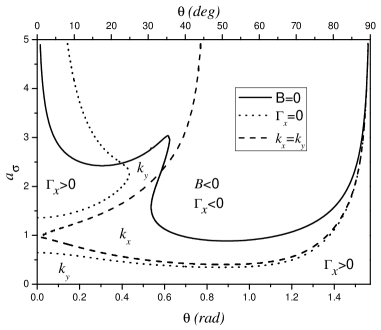
a)  b)

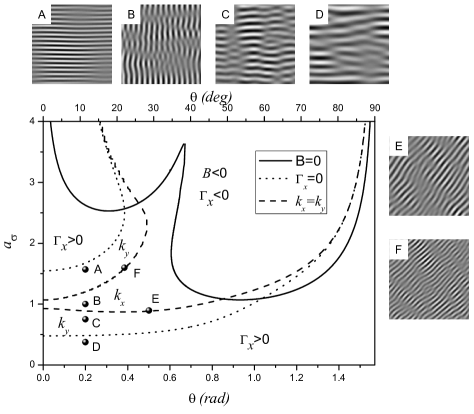
Figure 1: Phase diagrams for the pattern selection at in the system with multiplicative noise with $\Sigma=1$ (in domains denoted with $k_{\alpha}$ where $\alpha\in\{x,y\}$ patterns with wave-vector $\mathbf{k}=|k_{\alpha}|\hat{\alpha}$ are selected; plots (a), (b) correspond to $r_{c}=0.65$, $r_{c}=1$, respectively).

Next, we calculate the selected wave-lengths $\lambda_{x}$ and $\lambda_{y}$ versus the angle of incidence $\theta$ and the penetration depth $a_{\sigma}$ (Fig.2a) and versus the correlation scale $r_{c}$ and the energetic parameter $F$ (Fig.2b). The selected wave-lengths relate to the smallest wave-number in the corresponding direction. It is seen that as $a_{\sigma}$ or $\theta$ varies transformations in ripple orientation occur. Here $a_{\sigma i}$ and $\theta_{i}$ are threshold magnitudes for the penetration depth and incidence angle, respectively, indicating change of the ripple orientation. It is seen that there are two critical values $a_{\sigma 1}=a^{c}_{\sigma x}$ and $a_{\sigma 5}=a^{c}_{\sigma y}$ where the corresponding wave-lengths take infinitely large magnitudes due to $\Gamma_{x}=0$. There are two critical value for the angle $\theta_{2}=\theta_{x}^{c}$ and $\theta_{3}=\theta_{y}^{c}$ indicating divergence of the wave-lengths when $\Gamma_{x}$ takes zero values. From Fig.2b one can see that as the energetic parameter $F$ increases the wave-length of the ripple formation reduces to zero. At small $a_{\sigma}$ orientation of selected ripples can be changed at $F=F_{1}$, whereas at large values for the penetration depth no change is possible in the ripple orientation. The dependencies $\lambda_{\alpha}(r_{c})$ manifest non-monotonic behavior: at small $r_{c}$ the wave-length increases, whereas at large $r_{c}$ the decreasing dependencies are observed. Moreover, there is a critical value for the correlation radius $r_{c1}$ where orientation of ripples can be changed. Therefore, correlation properties of the ion beam can play a crucial role in ripple formation processes at early stages (in linear models). From the equations obtained for the selected wave-numbers it follows that the selected wave-lengths have the well-known assymptotics versus main parameters of the beam ($\lambda\sim T^{-1/2}\exp(-E_{a}/T)$, $\lambda\sim\epsilon^{-1/2}$, $\lambda\sim J^{-1/2}$) and depend assymptoticaly versus secondary characteristics: $\lambda\sim(\Sigma_{0}-\Sigma)^{1/2}$, $\lambda\sim(r_{c0}-r_{c})^{-1}$.

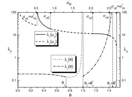
a) b)

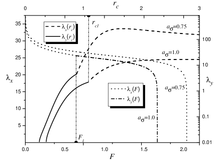
Figure 2: (a) Plot of selected wave-lengths $\lambda_{x}$ and $\lambda_{y}$ vs. incidence angle $\theta$ at $a_{\sigma}=0.45$, $r_{c}=0.65$ and dimensionless penetration depth $a_{\sigma}$ at $\theta=0.4763$, $r_{c}=1.0$ ($a_{\sigma i}$ with $i\in 1,\ldots,4$ denotes threshold values when a change of the wave-vector of patterns occurs); here $0<\theta<\pi/2$ is measured in radians; other parameters are: $F=1$, $\sigma=1$. (b) Plot of selected wave-lengths $\lambda_{x}$ and $\lambda_{y}$ vs. the correlation scale $r_{c}$ at $F=1.0$ and the energetic parameter $F$ at $r_{c}=1.0$ at $\theta=0.4763$. Other parameters are: $F=1$, $\sigma=1$, $\Sigma=1$.

4 Nonlinear stochastic model

Next, let us consider the nonlinear system behavior setting $\lambda_{\alpha}\neq 0$. In further study we are based on the simulation procedure allowing us to solve the nonlinear stochastic differential equation (4). As it was done in previous section we use the finite-difference approach to calculate the evolution of the field $h$.

4.1 Evolution of the height distribution function

To investigate properties of a distribution of the field $h$ we use skewness $m_{3}$ and kurtosis $m_{4}$, defined as

$$\begin{split}&m_{3}=\frac{\langle(h(\mathbf{r})-\langle{h}(\mathbf{r})\rangle)^{3}\rangle}{W^{3}},\\ &m_{4}=\frac{\langle(h(\mathbf{r})-\langle{h}(\mathbf{r})\rangle)^{4}\rangle}{W^{4}},\\ &W^{2}=\langle(h(\mathbf{r})-\langle{h}(\mathbf{r})\rangle)^{2}\rangle,\end{split}$$ (13)

where $\langle{h}(\mathbf{r})\rangle$ is the average of the height field ($\langle{h}(\mathbf{r})\rangle\equiv V^{-1}\sum_{\mathbf{r}}h(\mathbf{r},t)$, $V=L^{d}$ is the system volume, $d$ is the spatial dimension, $L$ is the linear size of the system); $W$ is the interface width. Skewness is a measure of the symmetry of a profile about the reference surface level. Its sign tells whether the father points are proportionately above ($m_{3}>0$) or below ($m_{3}<0$) the average surface level. Kurtosis describes randomness of the surface relative to that of a perfectly random (Gaussian) surface, for the Gaussian distribution one has $m_{4}=3.0$. Kurtosis is a measure of the sharpness of the height distribution function. It is known that if most of the surface features are concentrated near the mean surface level, then the kurtosis will be less than if the height distribution contained a larger portion of the surface features lying farther from the mean surface level.

a)
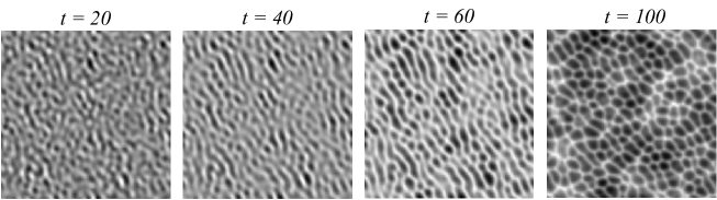
b)   c)

Figure 3: A typical evolution of the system with multiplicative fluctuations at early stages. (a) Snapshots of images of the field $h$ distribution for various growth times (dark color indicate low $h$, white areas relate to high $h$). b) Probability density function of the height for various growth time. c) Kurtosis, skewness, and interface width versus growth time. Other parameters are: $a_{\sigma}=1.2$, $\theta=0.4$, $F=1.0$, $\sigma=1.0$, $K=2.0$, $\Sigma=1.0$, $r_{c}=1.0$.

Figure 3a shows snapshots of the surface morphology for the set of parameters: $a_{\sigma}=1.2$, $\theta=0.4$, $F=1.0$, $\sigma=1.0$, $K=2.0$, $\Sigma=1.0$, $r_{c}=1.0$ at $t=20$, 40, 60, and 100, respectively. In our simulations we have used Gaussian initial conditions taking $\langle h(\mathbf{r},t=0)\rangle=0$, $\langle(\delta h)^{2}\rangle=0.1$; integration time step is $\Delta t=0.005$, space step is $\ell=1$. It is seen that with an increase of the growth time, the lateral length of the surface features becomes bigger and holes (black regions) are formed at $t=100$. It follows that due to nonlinear effects and noise action the surface morphology is crucially changed comparing to the ripples shown in Fig.1b. Figure 3b illustrates the corresponding height probability density distribution function of these surfaces. It is seen that at $t=20$ the distribution is close to the Gaussian distribution. With the increase of the growth time, there is deviation from zero-centered Gaussian distribution and after transient period of time the probability density function becomes symmetrical and centered around zero. In Fig.3c we plot the kurtosis $m_{4}$, the skewness $m_{3}$, and the interface width $W$ as functions of the growth time for above system parameters. According to initial conditions we have $m_{4}\simeq 3.0$, $m_{3}\simeq 0$ and $W\simeq 0$ at $t\simeq 0$. With the increase of the growth time the kurtosis grows until maximum is reached. The skewness decreases to its minimum, and after tends to zero. These two quantities reflect the form of the distribution function shown in Fig.3b. The interface width increases algebraically toward a saturation regime at large $t$.

We have computed phase diagram for the nonlinear systems illustrating formation of different patterns shown in Fig.4.

Figure 4: Phase diagram for the anisotropic nonlinear model at $F=1$, $\sigma=1$, $\Sigma=1$, $r_{c}=1$. Snapshots are taken at the system parameters related to position of the points $A$, $B$ and $C$, respectively.

It is seen that the numerical results are well related to analytical predictions from the linear stability analysis. Indeed, critical points lying on the lines correspond to a change of the sing of the quantity $\Gamma_{x}$. At large and low penetration depth $a_{\sigma}$ ripples oriented along $k_{y}$ direction are observed (see snapshot for the point $C$) due to $\Gamma_{x}>0$. At the intermediate values of $a_{\sigma}$ random patterns (holes) are realized due to the nonlinear influence of both the deterministic term $\lambda_{\alpha}(\nabla_{\alpha}h)^{2}$ and the stochastic contribution.

4.2 Scaling properties of the surface morphology

Using numerical data it is possible to study statistical properties of the system considering the time-dependent height-height correlation function, determined as follows $C_{h}(\mathbf{r},t)=\langle(h(\mathbf{r}+\mathbf{r}^{\prime},t)-{h}(\mathbf{r}^{\prime},t))^{2}\rangle$. In the framework of dynamic scaling hypothesis one can write the correlation function in the form [31, 32]

$$C_{h}(\mathbf{r},t)=2W^{2}(t)\phi\left(\frac{r}{\xi(t)}\right)$$ (14)

where

$$\phi(u)\sim\begin{cases}u^{2\alpha},&\text{for}\ \ u\ll 1,\\ \text{const},&\text{for}\ \ u\gg 1.\end{cases}$$ (15)

Early stages can be fitted by the function [33] $C_{h}(\mathbf{r},t)\approx 2W^{2}(t)[1-\exp[-(r/\xi)^{2\alpha}]$. The dynamic scaling hypothesis assumes that the following dependencies are hold: $W^{2}(t)\propto t^{2\beta}$, $\xi(t)\propto t^{1/z}$, where $\beta$ is the growth exponent, $z$ is the dynamic exponent for which $z=\alpha/\beta$. From another viewpoint one can assume [34]

$$C_{h}(\mathbf{r},t)=r^{2\alpha}\psi\left(\frac{t}{r^{z}}\right)$$ (16)

where

$$\psi(v)\sim\begin{cases}v^{2\beta},&\text{for}\ \ v\ll 1,\\ \text{const},&\text{for}\ \ v\gg 1,\end{cases}$$ (17)

and the relation $z=\alpha/\beta$ holds. Therefore, these two cases lead to the same results $C_{h}(t)\propto t^{2\beta}$ and $C_{h}(r)\propto r^{2\alpha}$, allowing one to define the growth exponent $\beta$ and the roughness exponent $\alpha$. As was shown in Ref.[34] the roughness $W(t,L)$ can be related to the structure function $S(\mathbf{k})$ as follows $W^{2}(t,L)=V^{-1}\sum_{\mathbf{k}\neq 0}S(\mathbf{k},t)$, where $S_{h}(k,t)=V^{-1}\langle h_{k}(t)h_{-k}(t)\rangle$. The structure function $S(k,t)$ has the form

$$S_{h}(k,t)=k^{-(d+2\alpha)}\Theta(k^{z}t),$$ (18)

where

$$\Theta(k^{z}t)\sim\begin{cases}k^{2\alpha}t^{2\alpha/\beta},&\text{for}\ \ k^{z}t\ll 1,\\ \text{const},&\text{for}\ \ k^{z}t\gg 1,\end{cases}$$ (19)

and scales as $S_{h}(k,t)\propto k^{-(d+2\alpha)}$ for large $t$ and $S_{h}(k,t)\propto t^{2\beta}$ for small $t$.

In previous studies (see, for example Ref.[6]) it was shown that even in the isotropic system with additive noise scaling exponents $\alpha$, $\beta$ and $z$ depend on the system parameters $\nu_{0}$, $\lambda_{0}$ and $K$. Moreover, these exponents are the time-dependent functions, i.e. its magnitudes can be changed in the course of the system evolution.

In our study we have taken into account multiplicative noise described by the energetic characteristics of the beam and additionally by the noise intensity $\Sigma$ and correlation radius of fluctuations $r_{c}$. Therefore, one should await that due to renormalization of the main system parameters responsible for the stability of the system and nonlinear effects in its behavior such scaling exponents are functions of the above noise properties. To prove it we compare magnitudes of both scaling exponents $\alpha$ and $\beta$ for the system with additive fluctuations and for the system with our multiplicative noise.

According to the scaling hypothesis the temporal evolution of the quantity $W=\langle(\delta h)^{2}\rangle$, where $\delta h=h-\langle h\rangle$, can be represented through the exponent $\delta$ related to the exponent $\beta$ as $\delta=\beta$. It is known that the ordinary diffusion (Brownian) process is described by Einshtein law $\langle(\delta h)^{2}\rangle\propto t^{2\delta}$, with $\delta=1/2$. If the exponent $\delta$ deviates from the value 1/2, then anomalous processes are realized: at $0<\delta<1/2$ there is a delayed (subdiffusion) process, whereas at $\delta>1/2$ the accelerated diffusion (superdiffusion) is realized. By comparison of results related to additive and multiplicative noise influence in anisotropic system, one can see that in the case of the additive noise influence we get $1/2<\delta<1$. In the case of the multiplicative noise influence the quantity $\delta$ takes values in the window $0<\delta<4$. It means that at small time intervals there are delayed processes which can be accelerated by the noise action at intermediate $t$; at large $t$ a transition toward saturation regime reduces growth velocity, decreasing $\delta$.

To characterize fractal properties of the surface one can study a pair correlation function defined as follows:

$$C_{p}(\mathbf{r};t)=\langle h(\mathbf{r}+\mathbf{r}^{\prime};t)h(\mathbf{r};t)\rangle.$$ (20)

If there is no characteristic space scale, then the introduced correlation function should behave itself algebraically, i.e., $C_{p}(r;t)\propto 1/r^{\Delta}$, where the scaling exponent $\Delta$ relates to the fractal correlation dimension $D_{2}$ as $\Delta=d-D_{2}$. The corresponding Fourier transformation of the correlation function $C_{p}(\mathbf{r};t)$ scales as $S_{p}(k;t)\propto k^{-D_{2}}$. From the definition of the correlation fractal dimension $D_{2}$ and the properties of the Fourier component of the correlator (20) it follows that at $D_{2}=0$ there is no scaling behavior of the structure function and $S_{p}(k;t)\approx const$. Hence, the surface at the fixed time $t$ can be considered as a Gaussian surface with no correlation, i.e. white noise in space with equal contribution of all wave-numbers $k$; the corresponding spatial correlator (20) is reduced to the Dirac delta-function, $C_{p}(\mathbf{r})\to\delta(\mathbf{r})$. In the case $D_{2}=2$ one arrives at typical dependence $S_{p}(k)\propto k^{-2}$ for diffuse spreading on the structured (let us say, flat) surface. Here the topological dimension $d$ equals the fractal dimension $D_{2}$. Therefore, a variation of the fractal dimension $D_{2}$ versus the time indicates a change of the fractal morphology of the surface from pure uncorrelated Gaussian surface toward well structured surface having fractal dimension $d=D_{2}=2$.

In order to study scaling properties of the system under consideration we will compare all our results obtained with results coming from an investigation of the anisotropic system with additive fluctuations. Such system will serve as a reference system. Moreover, to verify and to test our the numeric procedure of the scaling exponents computation we recalculate results of the work [6] for the isotropic Kuramoto-Sivashinsky equation.

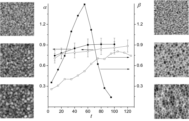
Figure 5: Roughness exponent $\alpha$ and growth exponent $\beta$ versus growth time for isotropic Kuramoto-Sivashinsky equation with additive noise (white circles and squares) at $\nu_{x}=\nu_{y}=-0.2$, $\lambda_{x}=\lambda_{y}=1.0$, $K=2$ and anisotropic Kuramoto-Sivashinsky equation with additive noise (black circles and squares) at $a_{\sigma}=1.2$, $\theta=0.4$ $K=2$. Snapshots are shown for above two models (left for isotropic and right for anisotropic Kuramoto-Sivashinsky equation with additive noise) at $t=20$, 60, 100 from top to bottom. The noise intensity $\Sigma=1.0$.

As a reference system we consider the model described by the Langevin equation with additive noise, i.e., $\partial_{t}h=\nu_{\alpha 0}\nabla_{\alpha\alpha}^{2}h+\frac{\lambda_{\alpha 0}}{2}(\nabla_{\alpha}h)^{2}-K\nabla^{2}(\nabla^{2}h)+\zeta(\mathbf{r},t)$, where $\zeta$ is the Gaussian random source with properties $\langle\zeta\rangle=0$, $\langle\zeta(\mathbf{r},t)\zeta(\mathbf{r}^{\prime},t^{\prime})\rangle=2\Sigma\delta(\mathbf{r}-\mathbf{r}^{\prime})\delta(t-t^{\prime})$. Calculations of the dynamical exponents at the system parameters $a_{\sigma}=1.2$, $\theta=0.4$, $F=1.0$, $\sigma=1.0$, $K=2.0$, $\Sigma=1.0$, $r_{c}=1.0$ are shown in Fig.5. It is seen that the exponents $\alpha$ and $\beta$ for above two models are different. In the anisotropic case we have elevated magnitudes for $\alpha$ and $\beta$, i.e. such exponents essentially depend on the control parameters of the system. Hence, due to renormalization of the control parameters by the multiplicative noise contribution the dynamic scaling exponents depend on the noise characteristics.

Let us consider the anisotropic system with multiplicative fluctuations. We have performed calculations of the scaling exponents at the fixed point on the phase diagram ($\theta$,$a_{\sigma}$) at different values of the noise intensity $\Sigma$ and the correlation radius $r_{c}$. The reference point is $a_{\sigma}=1.2$, $\theta=0.4$, $F=1.0$, $\sigma=1.0$, $K=2.0$. We compute $\alpha$ and $\beta$ at time window when the interface width $W$ or the correlation function $C_{h}(r)$ start to grow until they saturate (i.e., when algebraic dependencies $W^{2}(t)\propto t^{2\beta}$ and $C_{h}(r)\propto r^{2\alpha}$ are observed).

The corresponding time dependencies of $\alpha$, $\beta$ and $D_{2}$ are shown in Fig.6. In Fig.6a we plot the corresponding correlation function $C_{h}(r;t)$ and the roughness exponent $\alpha$; Figure 6b illustrates the time dependence of the interface width $W$ and the growth exponent $\beta$; Figure 6c shows the pair correlation function $C_{p}(r;t)$ and the associated fractal dimension $D_{2}$ at fixed times.

a)
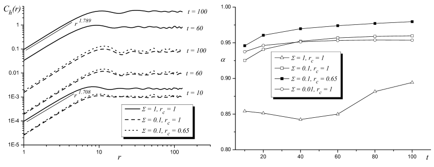
b)
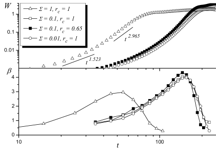
c)

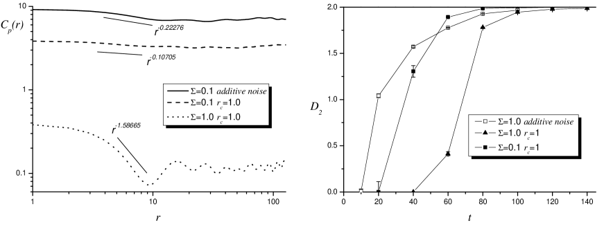
Figure 6: (a) The correlation function $C_{h}(r)$ and the roughness exponent $\alpha$ versus time. (b) The interface width $W$ and the growth exponent $\beta$ versus time. (c) The correlation function $C_{p}(r)$ at $t=60$ and the fractal dimension $D_{2}$ versus time. Other parameters are: $a_{\sigma}=1.2$, $\theta=0.4$, $F=1$, $\sigma=1$, $K=2$.

From Fig.6a it is seen that the growth process is nonstationary for early stages and the roughness exponent $\alpha$ is near 0.95 for small incidence angle dispersion $\Sigma$. At such set of the control parameters ($a_{\sigma}$ and $\theta$) the correlation radius $r_{c}$ has not essential influences on the system behavior. At large $\Sigma$ the roughness exponent has lower magnitudes and $\alpha$ has the well pronounced time dependence.

Comparing curves for the interface width at different $\Sigma$ and $r_{c}$ from the one hand and the growth exponents dependencies versus time from another one (see Fig.6b), one can conclude that as the noise intensity $\Sigma$ increases the position of the peak of the exponent $\beta$ reduces to small time. It means that as the noise intensity increases at such choice of the control parameters the interface width increases at smaller time interval than at low $\Sigma$. Alternatively, the shift of the peak position at large $\Sigma$ indicates that multiplicative fluctuations are responsible for nonlinear effects at small times. It looks natural due to the nonlinear form of the multiplicative noise, where the large noise contribution influences crucially on properties of the growth processes. The correlation properties of fluctuations characterized by $r_{c}$ define a height of the peak for $\beta$. In other words, the noise correlations can accelerate growth processes increasing the interface width $W$ until it attains the saturation.

A change of the fractal properties of the surface is shown in Fig.6c. Here we compare fractal properties of two different systems, namely with additive fluctuation source and with multiplicative noise. From the dependencies of the pair correlation function $C_{p}(r)$ it is seen that at $t=60$ the additive noise contribution leads to a picture when the correlation function $C_{p}(r)$ decreases slowly with exponent $\Delta=0.227$, whereas the multiplicative noise contribution with the same intensity $\Sigma=1.0$ at $r_{c}=1.0$ increases the exponent $\Delta$ to 1.587. According to the definition of the correlation dimension $D_{2}$ it means that the fractal properties of the surface is well pronounced at multiplicative noise with large intensity at a small time interval $t\simeq 60$ (see curves $D_{2}(t)$). From the time dependencies of the fractal dimension $D_{2}$ for the system with multiplicative noise it follows that at small times the surface has Gaussian properties of the kind of white noise in space (the correlation function has the from of the Dirac delta-function.). At small time interval (at intermediate times) the fractal properties emerge and characterized by $0<D_{2}<2$. At large times one has $D_{2}=2$ and the well structured patterns are observed, its dimension $D_{2}$ coincides with the topological $d=2$. In the case of additive fluctuations the time interval of the formation of well structured patterns is larger than in system with multiplicative noise.

a)
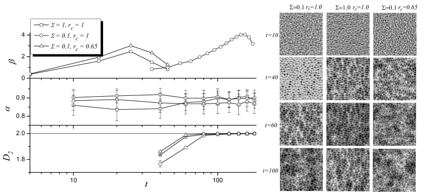
b)

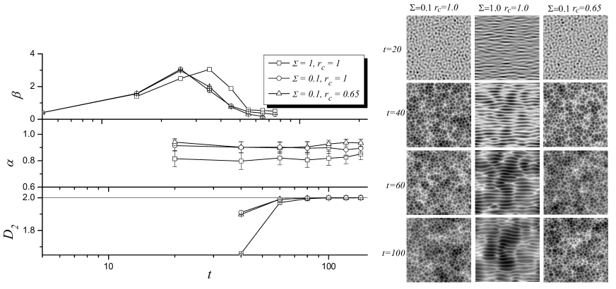
Figure 7: Scaling exponents $\alpha$, $\beta$ and correlation dimension $D_{2}$ versus time at (a) $a_{\sigma}=2.0$, $\theta=0.4$ and (b) $a_{\sigma}=2.0$, $\theta=0.2$. Typical snapshots of the system evolution are taken at different $\Sigma$ and $r_{c}$. Other parameters are: $F=1$, $\sigma=1$, $K=2$

Next let us compare the time dependencies for the scaling exponents for different set of the system parameters $a_{\sigma}$ and $\theta$ shown in Figs.7a,b. It is seen that at $a_{\sigma}=2.0$, $\theta=0.4$ (Fig.7a) at large noise intensity $\Sigma$ the interface width grows faster comparing with the case of small $\Sigma$ at fixed $r_{c}$. But the growth at small $\Sigma$ occurs at earlier periods of time. This situation absolutely different to the case shown in Fig.6b, whereas variations in $r_{c}$ leads to the increase of the maximum for $\beta$. The roughness exponent $\alpha$ does not principally change its values at different $t$. Comparing curves for the fractal dimension $D_{2}$ for above two sets of the system parameters one can see that at small $\Sigma$ the quantity $D_{2}$ is smaller than in previous case (cf. dependencies $D_{2}(t)$ in Figs.6c, 7a). The same dependencies of the scaling exponent $\alpha$, $\beta$ and $D_{2}$ at $a_{\sigma}=2.0$, $\theta=0.2$ are observed. Here at large $\Sigma$ the nonlinear effects delayed. Considering snapshots shown in the right hand side of the plots at different $\Sigma$ and $r_{c}$ one can see that depending on the noise properties the morphology of the surface changes crucially (cf. snapshots at different $r_{c}$ in Fig.7b). It means that the phase diagram shown in Fig.4 will be modified under variation of $\Sigma$ or $r_{c}$ as linear stability analysis predicts.

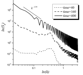
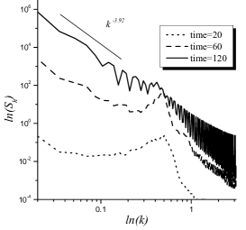
a) b) c)

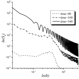
Figure 8: Evolution of the spherically averaged structure function $S_{h}(k,t)$ at different noise intensity: a) $\Sigma=0.1$, $r_{c}=1$; b) $\Sigma=1.0$, $r_{c}=1$; c)$\Sigma=0.1$, $r_{c}=0.65$. Other parameters are: $a_{\sigma}=1.2$, $\theta=0.4$, $F=1$, $\sigma=1$.

Figure 8 show the evolution of the spherically averaged structure function defined on a circle

$$S_{h}(k,t)=\frac{1}{N_{k}}\sum\limits_{k\leq\mathbf{k}\leq k+\Delta k}S_{h}(\mathbf{k},t),$$ (21)

where $N_{k}$ is the number of point on the circle of the width $\Delta k$. Two different choice of the noise intensity $\Sigma$ and the correlation radius of fluctuations $r_{c}$ are shown in Figs.8a,b,c, respectively. It is seen that during the system evolution at early stages the system selects the ripples with the corresponding wave-number (dotted lines) and after at late stages the algebraic form for the structure function is realized. At large time intervals one can define the exponent $\alpha$ from the definition $S_{h}(k)\propto k^{-(d+2\alpha)}$. As is shown in Figs.8a,b for above system parameters one has $S_{h}(k)\propto k^{-3.86}$ for $\Sigma=0.1$ and $S_{h}(k)\propto k^{-3.92}$ for $\Sigma=1.0$, where $d=2$. Hence, the roughness exponent takes values $\alpha\simeq 0.93$ and $\alpha\simeq 0.96$ that is well predicted by the analysis of the correlation function $C_{h}(r)$ (see Figs.6a).

5 Conclusions

We have studied the ripple formation processes induced by the ion sputtering under stochastic conditions of illumination. The main assumption was stochastic nature of the ion beam when the angle of incidence distributed in space and time (homogeneous and stationary field). It allows us to generalize the Bradley-Harper model of ripple formation [3] and consider the stochastic model with multiplicative fluctuations describing random nature of the incidence angle proposed in Ref.[9]. We have discussed properties of the ripple formation in both linear and nonlinear models.

Within the framework of the linear stability analysis we have shown that even in the linear system the noise action is able to change the critical values for the control parameters of the system such as the penetration depth and the averaged incidence angle. It was found that as correlation properties of such multiplicative noise as the dispersion in the incidence angles around the average can reduce the domains of the control parameters where the ripples change their orientation at the fixed angle of incidence.

Studying the nonlinear model we have computed the dynamic phase diagram illustrating formation of different patterns (ripples and holes) which relates to the results from the linear stability analysis. Main properties of the ripple formation were studied with the help of the distribution function of the height and its averages reduced to the skewness, kurtosis and interface width (dispersion). To make a detailed analysis of the ripple formation we have examined scaling behavior of main statistical characteristics of the system reduced to the correlation functions and its Fourier transforms (structure functions). It was shown that as the growth and roughness exponents depend on the control parameters and are time-dependent functions (it was predicted by previous study of the isotropic Kuromoto-Sivashinsky equation [6]); these exponents depend on the noise properties: its intensity and the spatial correlation radius. Comparing results for the system with additive and multiplicative fluctuations it was shown that multiplicative noise can crucially accelerate processes of ripple formation, increasing the growth exponent. As far as our system is anisotropic the noise action is different at different set of the main control parameter values. Studying fractal properties of the surface we have calculated the fractal (correlation) dimension as the time-dependent function. It was shown that in the system with multiplicative noise the fractal properties appear at small time interval of the surface growth, whereas in the system with the additive noise this time interval is wider. These results are well predicted by the correlation functions analysis and by Fourier transformation of the numerically calculated surface.

Therefore, as patterning as the scaling behavior of the system can be controlled by additional set of parameters reduced to the dispersion of the angle of incidence and the correlation properties of its fluctuations.

References

- [1] L.Jacak, P.Hawrylak, A.Wojs, Quantum Dots, Springer-Verlag, Berlin, 1998
- [2] M.Navez, C.Sella, D.Chaperot, Ionic Bombardment: Theory and Applications, ed.by J.J.Trillat, Gordon and Breach, New York, 1964.
- [3] R.M.Bradley, J.M.E.Harper, J.Vac.Sci.Technol.A, 6(4), 2390, (1988)
- [4] R.Cuerno, A.-L.Barabasi, Phys.Rev.Lett., 74, 23, 4746 (1995)
- [5] M.Makeev, A.-L.Barabasi, Appl.Phys.Lett, 71, 2800 (1997)
- [6] J.T.Drotar, Y.-P.Zhao, T.-M.Lu, G.-C.Wang,Phys.Rev.E, 59, 177, (1999)
- [7] T.Aste, U.Valbusa, Physica A, 332, 548, (2004)
- [8] B.Kahng, J.Kim, Curr.Appl.Phys., 4, 115, (2004)
- [9] R.Kree, T.Yasseri, A.K.Hartmann, NIMB, 267, 1407 (2009)
- [10] S.Rusponi, C.Boragno, U.Valbusa, Phys.Rev.Lett., 78, 2795 (1997)
- [11] S.Rusponi, G.Costantini, C.Boragno, U.Valbusa, Phys.Rev.Lett., 81, 2735 (1998)
- [12] E.Chason, T.M.Mayer, B.K.Kellerman, et al., Phys.Rev.Lett., 72 2040 (1994)
- [13] J.Erlebacher, M.J.Aziz, E.Chason, et al., Phys.Rev.Lett., 82 2330 (1999)
- [14] W.-Q.Li, L.J.Qi, X.Yang, et al., Appl.Surf.Sci., 252, 7794 (2006)
- [15] W.J.MoberlyChan, D.P.Adams, M.J.Aziz, et al., MRS Bulletin, 32, 424 (2007)
- [16] H.X.Qian, W.Zhou, Y.Q.Fu, et al., Appl.Surf.Sci., 240, 140 (2005)
- [17] D.Paramanik, S.Majumdar, S.R.Sahoo et al., Jour.Nanosci.and Nanotech, 8, 1 (2008)
- [18] J.Lian, Q.M.Wei, L.M.Wang et al., Appl.Phys.Lett., 88, 093112 (2006)
- [19] S.Facsko, T.Dekorsy, C.Koerdt et al., Science, 285, 1551 (1999)
- [20] M.Kardar, G.Parisi, Y.-C.Zhang, Phys.Rev.Lett., 56, 889, (1986)
- [21] D.E.Wolf, J.Villian, Europhys.Lett., 13(5), 389 (1990)
- [22] Y.Kuramoto, T.Tsuzuki, Prog.Theor.Phys., 55, 356 (1977); G.I.Sivashinsky, Acta Astronaut., 6, 569 (1979)
- [23] B.Ziberi, F.Frost, M.Tartz, et al., Appl.Phys.Lett., 92, 063102 (2008)
- [24] P.Sigmund, J.Matter.Sci, 8, 1545 (1973)
- [25] M.A.Makeev, A.-L.Barabasi, NIMB, 222, 316 (2004)
- [26] P.Sigmund, Phys.Rev., 184, 383 (1969)
- [27] J.W.Cahn, J.E.Taylor, ActaMetall.Matter, 42, 1045 (1994)
- [28] C.W.Gardiner, Handbook of Stochastic Methods, Springer-Verlag, Berlin, Heidelberg, New-York, Tokyo, 1985.
- [29] J. Garcia–Ojalvo, J.M. Sancho, Noise in Spatially Extended Systems, Springer, New York, 1999.
- [30] E.A. Novikov, Zh. Eksp. Teor. Fiz. 47 (1964) 1919. English Translation, Sov. Phys. JETP 20 (1965) 1290.
- [31] F.Family, T.Vicsek, J.Phys.A, 18, L75, (1985)
- [32] F.Family, Physica A, 168, 561, (1990)
- [33] S.K.Sinha, E.B.Sirota, S.Garott, Phys.Rev.B, 38, 2297 (1988)
- [34] L.Giada, A.Giacometti, M.Rossi, Phys.Rev.E, 65, 036134 (2002)