The influence of line tension on the formation of liquid bridges

Abstract

The formation of liquid bridges between a planar and conical substrates is analyzed macroscopically taking into account the line tension. Depending on the value of the line tension coefficient $\tau$ and geometric parameters of the system one observes two different scenarios of liquid bridge formation upon changing the fluid state along the bulk liquid-vapor coexistence. For $\tau>\tau^{*}$ ($\tau^{*}<0$) there is a first-order transition to a state with infinitely thick liquid bridge. For $\tau<\tau^{*}$ the scenario consists of two steps: first there is a first-order transition to a state with liquid bridge of finite thickness which upon further increase of temperature is followed by continuous growth of the thickness of the bridge to infinity. In addition to constructing the relevant phase diagram we examine the dependence of the width of the bridge on thermodynamic and geometric parameters of the system.

I Introduction

In this note we investigate the phase diagram of a fluid enclosed between two infinite walls: one planar and one conical. Such a system resembling the atomic force microscope geometry has been analyzed in different contexts Butt et al. (2005, 2003); Jang et al. (2002). Particular emphasis has been put on the structure of the phase diagram which displays a phase characterized by the presence of a liquid bridge formed between the walls Dutka and Napiórkowski (2007).

The mean curvature of the meniscus of the bridge is given by the Young-Laplace equation Rowlinson and Widom (1982) and its width is a function of the undersaturation Jang et al. (2002, 2004). The presence of the bridge induces force acting between opposite walls which can be measured using atomic force microscope Butt and Kappl (2009); Butt et al. (2003). It turns out, however, that the line tension can have qualitative influence on the phase behavior of such system. This issue has not received much attention in the literature and we discuss it in this note. In particular, we focus on bridge formation and filling transitions along the bulk liquid-vapor coexistence where presence of line tension leads to effects similar to what - in a different context - is termed a frustrated complete wetting [][andreferencestherein.]Bonn1.

In the following section we recall the form of the free energy functional of the shape of liquid bridge. This functional and the corresponding equation for equilibrium liquid-vapor interfacial shape supplemented by the boundary conditions form the basis of our approach. Their analysis along the bulk liquid-vapor coexistence for different values of the line tension coefficient leads to different transition scenarios presented in Section III. In the last section we summarize our results and point at the possibility of indirect measurement of the width of the bridge. The behavior of this width reflects the transition scenario taking place in the system.

II Shape of a liquid bridge

The system under considerations consists of a fluid confined between two walls, Fig. 1. The thermodynamic state of the fluid is located on the bulk liquid-vapor coexistence line.

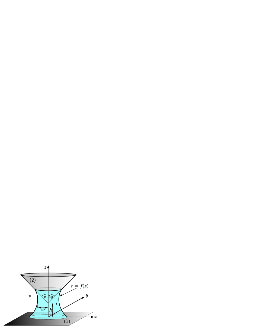
Figure 1: A liquid-like bridge ($l$) surrounded by vapor ($v$) connects the planar $(1)$ and conical $(2)$ walls.

The surface of the lower substrate $(1)$ is an infinite plane $z=0$, and the upper substrate $(2)$ is formed by infinite cone whose tip is at distance $h$ from the plane $z=0$. The system is axially symmetric around the $z$-axis. In cylindrical coordinates $(r=\sqrt{x^{2}+y^{2}},z\geqslant 0)$ the surface of the cone is described by $r=a(z)=(z-h)\cot\varphi$, where $z\geqslant h$ and $\pi-2\varphi$ is the opening angle of the cone ($0\leqslant\varphi\leqslant\pi/2$). In our macroscopic approach the grand canonical functional $\Omega([f],T,h,\varphi)$ is a functional of the liquid-vapor interfacial shape $r=f(z)$. It is parametrized by the temperature $T$ and by geometric parameters $h$ and $\varphi$. Instead of temperature we shall use the angle $\theta$ which fulfills the Young equation Rowlinson and Widom (1982). The actual contact angles present in the problem fulfill the modified Young equations Swain and Lipowsky (1998) but it is convenient to use $\Theta$ to reparametrize the temperature dependence. We assume that both substrates are made of the same material and are thus characterized by the same angles $\theta_{1}=\theta_{2}=\theta$, and the same line tension coefficients $\tau_{1lv}=\tau_{2lv}=\tau$. Accordingly, $\cos\theta=(\sigma_{sv}-\sigma_{sl})/\sigma_{lv}$, where $\sigma_{\alpha\beta}$ denote the relevant surface tension coefficients. Although for a given system both the line and surface tension coefficients are functions of its thermodynamic state, in our macroscopic analysis they will be varied independently. In other words, the parameters $\theta$ and $\tau$ will be considered as independent variables. In particular, the possibility of both signs of $\tau$ will be taken into account.

At bulk liquid-vapor coexistence the functional of the liquid bridge shape $f(z)$ relative to the state without the bridge $\Delta\Omega[f]$ is given by Dutka and Napiórkowski (2007):

$$\frac{\Delta\Omega[f]}{2\pi\sigma_{lv}}=\int dz\,\Theta(f-a)\Big{\{}f\sqrt{1+f^{\prime 2}}\,\Theta(f)\,\Theta(z)$$

$$-\cos\theta\Big{[}\frac{f^{2}}{2}\,\delta(z)+\frac{a}{\sin\varphi}\,\Theta(z-h)\,\Big{]}$$

$$+\tilde{\tau}\,\Big{[}f\,\delta(z)+\cot\varphi\,\Theta(z-h)\,\Big{]}\Big{\}},$$ (1)

where the ratio $\tilde{\tau}=\tau/\sigma_{lv}$ has dimension of length. The symbols $\Theta(z)$ and $\delta(z)$ denote the Heaviside and Dirac function, respectively.

The equilibrium interfacial shape $\bar{f}(z)$ minimizes $\Delta\Omega[f]$. This leads to equation

$$\frac{1}{\bar{f}(z)\sqrt{1+\bar{f}^{\prime}(z)^{2}}}-\frac{\text{d}}{\text{d}z}\frac{\bar{f}^{\prime}(z)}{\sqrt{1+\bar{f}^{\prime}(z)^{2}}}=0$$ (2)

and two boundary conditions

$$\begin{split}0=&\Bigg{[}\cos\theta+\frac{\bar{f}^{\prime}(z)}{\sqrt{1+\bar{f}^{\prime}(z)^{2}}}-\frac{\tilde{\tau}}{\bar{f}(z)}\Bigg{]}\Bigg{|}_{z=0}\,,\\ 0=&\Bigg{[}\cos\theta-\frac{\sin\varphi+\cos\varphi\bar{f}^{\prime}(z)}{\sqrt{1+\bar{f}^{\prime}(z)^{2}}}-\frac{\tilde{\tau}}{\bar{f}(z)}\cos\varphi\Bigg{]}\Bigg{|}_{z=z_{2}}\,.\end{split}$$ (3)

The above boundary conditions are equivalent to the modified Young equations for each of the substrates. The coordinate $z_{2}$ is such that $\bar{f}(z_{2})=a(z_{2})$. The lhs of (2) is equal to the mean curvature of the interface and thus the surface of the bridge is a catenoid. The solution of (2)

$$\bar{f}(z)=w\cosh\frac{z-z_{1}}{w}\,,$$ (4)

is parametrized by $z_{1}$ and $w$, where $w=\bar{f}(z_{1})$ is the minimal value of $\bar{f}$ which will be considered to be the width of the bridge. With the help of dimensionless quantities $\alpha=z_{1}/w$ and $\beta=z_{2}/w$ the boundary conditions (3) can be rewritten as

$$\cos\theta= \,\frac{\tilde{\tau}}{w\cosh\alpha}+\tanh\alpha\,,$$ (5)

$$\cos\theta= \,\frac{\tilde{\tau}\cos\varphi}{w\cosh(\beta-\alpha)}+\frac{\sin\varphi}{\cosh(\beta-\alpha)}+\tanh(\beta-\alpha)\cos\varphi\,.$$ (6)

Now the width of the bridge $w$ can be considered to be the following function of $\alpha$ and $\beta$ parametrized by $h$ and $\varphi$:

$$w(\alpha,\beta)=\frac{h}{\beta-\tan\varphi\cosh(\beta-\alpha)}\ .$$ (7)

The relative free energy of the system is given by

$$\Delta\bar{\Omega}=\pi\sigma_{lv}\,h\,w(\alpha,\beta)\Big{[}\frac{\tilde{\tau}}{h}\Big{(}\cosh\alpha+\cosh(\beta-\alpha)\Big{)}+1\Big{]}\,.$$ (8)

Analysis of the above equation enables the construction of the phase diagram; this will be discussed in the next section.

III Phase diagram

The basis for determining the phase diagram is the knowledge of the equilibrium shapes of the bridge $f=\bar{f}(z)$ and the corresponding relative grand canonical free energies $\Delta\bar{\Omega}=\Delta\Omega[\bar{f}]$. Depending on the sign of $\Delta\bar{\Omega}$ three cases are possible: (a) $\Delta\bar{\Omega}<0$ – the phase with the bridge present is favorable, (b) $\Delta\bar{\Omega}>0$ – phase without bridge is favorable, (c) $\Delta\bar{\Omega}=0$ – the previous phases coexist.

The set of equations (5) and (6) is not solvable analytically. The numerically obtained plots of functions $\beta=\beta(\alpha)$ (parametrized by $\theta$, $\tilde{\tau}$, $h$ and $\varphi$) illustrate the transition scenario taking place at bulk liquid-vapor coexistence, Fig. 2, for fixed value of the opening angle of the cone, $\varphi=\pi/6$, and negative value of the line tension coefficient $\tilde{\tau}=-h$. For the angles $\theta>\theta^{*}(\tilde{\tau}/h,\varphi)$ the curves corresponding to the solutions of equations (5) and (6) do not intersect, Fig. 2a. This situation corresponds to the absence of the liquid bridge. For $\theta=\theta^{*}(\tilde{\tau}/h,\varphi)$, Fig. 2b, the bridge with a finite width is present, and its relative free energy $\Delta\bar{\Omega}$ is negative. For $\theta^{*}_{0}(\varphi)<\theta<\theta^{*}(\tilde{\tau}/h,\varphi)$ there are two solutions of (5) and (6) with negative relative free energies corresponding to bridges of different width $w(\alpha,\beta)$. The solution with a larger width is represented by point $A$ on Fig. 2c and has smaller energy than the one corresponding to point $B$. Upon decreasing the angle $\theta$ towards the angle $\theta=\theta^{*}_{0}(\varphi)$ the width of the bridge tends to infinity, Fig. 2d. For $\theta\leqslant\theta^{*}_{0}(\varphi)$ the bridge has infinite width which corresponds to the whole space between the walls filled with liquid.

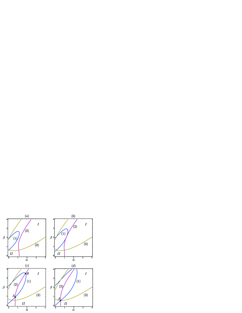
Figure 2: Plots of functions $\beta=\beta(\alpha)$ obtained by numerically solving equations (5) and (6), curves $(1)$ and $(2)$, respectively. Different values of angle $\theta$ are considered: (a) $\theta>\theta^{*}(\tilde{\tau}/h,\varphi)$, (b) $\theta=\theta^{*}(\tilde{\tau}/h,\varphi)$, (c) $\theta^{*}_{0}(\varphi)<\theta<\theta^{*}(\tilde{\tau}/h,\varphi)$, (d) $\theta=\theta^{*}_{0}(\varphi)$ at fixed $\tilde{\tau}=-h$ and $\varphi=\pi/6$. The curve denoted as $(3)$ corresponds to $w(\alpha,\beta)^{-1}=0$, and divides the $(\alpha,\beta)$ plane into part corresponding to $w(\alpha,\beta)>0$ (denoted as $I$), and (unphysical) part corresponding to $w(\alpha,\beta)<0$ (denoted as $II$). Points of intersection $A$ and $B$ correspond to equilibrium solutions; point $A$ is the solution which corresponds to the bridge with a larger width and smaller relative free energy.

For particular value of the angle $\theta=\theta^{*}_{0}(\varphi)$ the width of the bridge becomes infinite, and equations (5) and (6) do not depend on the line tension coefficient $\tilde{\tau}$. Their solutions denoted by $\alpha^{*}$ and $\beta^{*}$ have the following form

$$\begin{split}\alpha^{*}=&\,\arccos\!\text{h}\frac{1}{\sin\theta^{*}_{0}}\ ,\\ \beta^{*}=&\,\arccos\!\text{h}\frac{1}{\sin(\theta^{*}_{0}+\varphi)}+\arccos\!\text{h}\frac{1}{\sin\theta^{*}_{0}}\,.\end{split}$$ (9)

After inserting the above expressions to equation $w(\alpha^{*},\beta^{*})^{-1}=0$ one gets the equation for the angle $\theta^{*}_{0}(\varphi)$

$$\arccos\!\text{h}\frac{1}{\sin(\theta^{*}_{0}+\varphi)}+\arccos\!\text{h}\frac{1}{\sin\theta^{*}_{0}}=\frac{\tan\varphi}{\sin(\theta^{*}_{0}+\varphi)}\,.$$ (10)

Its numerical solution is shown on Fig. 3. For $\varphi\ll 1$ the function $\theta^{*}_{0}$ can be approximated by $\theta^{*}_{0}\simeq\pi/2-\varphi$, and for $\varphi\to\pi/2$ it tends to zero tangentially.

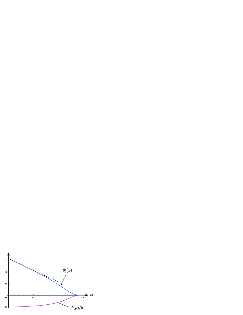
Figure 3: The dependence of the angle $\theta^{*}_{0}$ and the dimensionless line tension coefficient $\tilde{\tau}^{*}/h$ on the opening angle $\varphi$ (solid lines). For $\varphi\ll 1$ the function $\theta^{*}_{0}(\varphi)$ can be approximated by $\theta^{*}_{0}\simeq\pi/2-\varphi$ and the line tension coefficient by $\tilde{\tau}^{*}/h\simeq-0.5$ (dashed lines). For $\varphi\to\pi/2$ both functions tend to zero tangentially.

We note that the bridge of finite width can exist for $\theta>\theta^{*}_{0}(\varphi)$ provided the free energy of the system (8) evaluated at $\theta=\theta^{*}_{0}(\varphi)$ is not greater than zero. This requirement can be rewritten as the condition on the line tension coefficient

$$\tilde{\tau}\leqslant-h\,\frac{\sin\theta^{*}_{0}(\varphi)\sin(\theta^{*}_{0}(\varphi)+\varphi)}{\sin\theta^{*}_{0}(\varphi)+\sin(\theta^{*}_{0}(\varphi)+\varphi)}\equiv\tilde{\tau}^{*}(\varphi)\,.$$ (11)

Thus for $\tilde{\tau}\leqslant\tilde{\tau}^{*}(\varphi)$ the liquid bridge is present for $\theta\geqslant\theta^{*}_{0}(\varphi)$, otherwise there is no bridge in the system. For $\varphi\ll 1$ the line tension coefficient can be approximated by the function $\tilde{\tau}^{*}/h\simeq-0.5$, and for $\varphi\to\pi/2$ tends to zero tangentially, Fig. 3.

In order to find the divergence of the width of the bridge for $\theta\to\theta^{*}_{0}(\varphi)$ at fixed $\tilde{\tau}<\tilde{\tau}^{*}(\varphi)$ we expand equations (5) and (6) around $\theta=\theta^{*}_{0}(\varphi)$, $\alpha=\alpha^{*}$ and $\beta=\beta^{*}$. In the leading order the divergence is given by

$$w\simeq A(\varphi)\,h\,\frac{\tilde{\tau}^{*}(\varphi)-\tilde{\tau}}{|\tilde{\tau}^{*}(\varphi)|}\,\Big{[}\theta-\theta^{*}_{0}(\varphi)\Big{]}^{-1}\,,$$ (12)

where the amplitude

$$A(\varphi)=\frac{\sin^{2}(\theta^{*}_{0}(\varphi)+\varphi)\,\sin\theta^{*}_{0}(\varphi)\,\cos\varphi}{\sin^{2}(\theta^{*}_{0}+\varphi)+\sin^{2}\theta^{*}_{0}(\varphi)}$$ (13)

is positive for $0<\varphi<\pi/2$.

To find the angle $\theta=\theta^{*}(\tilde{\tau}/h,\varphi)$ at which there is a first order transition from the phase without bridge to phase with the bridge one has to solve eqs. (5), (6), (7) supplemented by the requirement of tangetiality of the curves $\beta(\alpha)$ determined by these equations, Fig.2b. The numerically obtained phase diagram, Fig. 4, displays the coexistence line between the phase with no bridge in the system $(NB)$ and with the bridge $(B)$. The coexistence lines for $\tilde{\tau}\leqslant\tilde{\tau}^{*}$ and for $\tilde{\tau}\geqslant\tilde{\tau}^{*}$ meet tangentially. For $\theta^{*}_{0}<\theta\leqslant\theta^{*}$ the width of the bridge is finite $(w<\infty)$ and for $\theta\leqslant\theta^{*}_{0}$ the whole system is filled with the liquid phase $(w=\infty)$.

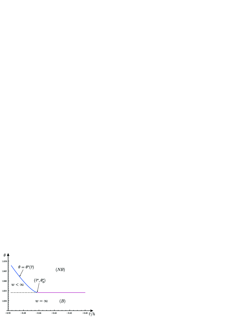
Figure 4: The phase diagram in variables $(\tilde{\tau}/h,\theta)$ displaying the coexistence line between the phase with no liquid bridge present in the system $(NB)$ and with the bridge present in the system $(B)$ (continuous line), $(w<\infty)$ denotes the region in which the width of the bridge is finite, and $(w=\infty)$ – the region where the whole system is filled with liquid. The opening angle is equal $\varphi=\pi/6$, for which $\theta^{*}_{0}\approx 1.034$ and $\tilde{\tau}^{*}/h\approx-0.462$.

IV Discussion

We have shown that a fluid confined between planar and a conical walls may undergo – upon changing its thermodynamic state along the bulk liquid-vapor coexistence line – two different transition scenarios leading from the phase without liquid bridge to the phase with liquid bridge of infinite thickness. The type of scenario depends on the value of dimensionless line tension coefficient $\tau/\sigma_{lv}h\equiv\tilde{\tau}/h$. For $\tilde{\tau}<\tilde{\tau}^{*}(\varphi)$ first the bridge of finite width is formed discontinuously at temperature corresponding to angle $\theta=\theta^{*}(\tilde{\tau}/h,\varphi)$. Upon further decrease of $\theta$ the width of the bridge increases continuously and at $\theta=\theta^{*}_{0}(\varphi)$ it becomes infinite; the whole space between substrates is filled with the liquid phase. This scenario is qualitatively similar to the one observed experimentally by Takata et al.Takata et al. (2008) in a different context. On the other hand, when decreasing the angle $\theta$ at $\tilde{\tau}>\tilde{\tau}^{*}(\varphi)$ one observes a discontinuous transition at $\theta=\theta^{*}_{0}(\varphi)$. This transition takes the system from the phase without the liquid bridge to the phase with bridge of infinite width.

To find the width of the bridge one can perform the solvation force measurements using the atomic force microscope Butt et al. (2005, 2003); Jang et al. (2002) with conical tip. The solvation force associated with the liquid bridge $F=-\partial\Delta\bar{\Omega}(T,h,\varphi)/\partial h$ can be rewritten in the following $z$-independent form

$$F=-2\pi\sigma_{lg}\,\frac{\bar{f}(z)^{2}}{2}\left[\frac{1}{r_{1}(z)}+\frac{1}{r_{2}(z)}\right]\,,$$ (14)

where the radii of curvature

$$\begin{split}r_{1}(z)=&\,\left[\frac{{\rm d}}{{\rm d}z}\frac{\bar{f}^{\prime}(z)}{\sqrt{1+\bar{f}^{\prime}(z)^{2}}}\right]^{-1}\,,\\ r_{2}(z)=&\,\bar{f}(z)\sqrt{1+\bar{f}^{\prime}(z)^{2}}\,,\end{split}$$ (15)

can be evaluated at arbitrary $z\in[0;z_{2}]$. The $z$-independent expression in (14) can be presented in a particularly transparent form Farshchi-Tabrizi et al. (2006)

$$F=-2\pi\sigma_{lg}w\,,$$ (16)

where the negative sign indicates that the substrates attract each other once the liquid bridge is formed. Thus the solvation force measurements provide direct information on the width of the liquid bridge.

References

- Butt et al. (2005) H. Butt, B. Capella, and M. Kappl, Surf. Sci. Rep., 59, 1 (2005).
- Butt et al. (2003) H. J. Butt, K. Graf, and M. Kappl, Physics and chemistry of interfaces (Wiley-VCH, Weinheim, 2003).
- Jang et al. (2002) J. Jang, G. C. Schatz, and M. A. Ratner, J. Chem. Phys., 116, 3875 (2002).
- Dutka and Napiórkowski (2007) F. Dutka and M. Napiórkowski, J. Phys.: Condens. Matter, 19, 466104 (2007).
- Rowlinson and Widom (1982) J. S. Rowlinson and B. Widom, Molecular Theory of Capillarity (Oxford University, London, 1982).
- Jang et al. (2004) J. Jang, G. C. Schatz, and M. A. Ratner, Phys. Rev. Lett., 92, 885504 (2004).
- Butt and Kappl (2009) H. J. Butt and M. Kappl, Advances in Colloid and Interface Science, 146, 48 (2009).
- Bonn et al. (2009) D. Bonn, J. Eggers, J. O. Indekeu, J. Meunier, and E. Rolley, Rev. Mod. Phys., 81, 739 (2009).
- Swain and Lipowsky (1998) P. S. Swain and R. Lipowsky, Langmuir, 14, 6772 (1998).
- Takata et al. (2008) Y. Takata, H. Matsubara, T. Matsuda, Y. Kikuchi, T. Takiue, B. Law, and M. Aratono, Colloid & Polymer Science, 286, 647 (2008).
- Farshchi-Tabrizi et al. (2006) M. Farshchi-Tabrizi, M. Kappl, Y. Cheng, J. Gutmann, and H. J. Butt, Langmuir, 22, 2171 (2006).