The Generation, Evolution and Decay of Pure Quantum Turbulence: A Full Biot-Savart Simulation

Abstract

A zero temperature superfluid is arguably the simplest system in which to study complex fluid dynamics, such as turbulence. We describe computer simulations of such turbulence and compare the results directly with recent experiments in superfluid ³He-B. We are able to follow the entire process of the production, evolution, and decay of quantum turbulence. We find striking agreement between simulation and experiment and gain new insights into the mechanisms involved.

The tangle of similar quantized vortices in a pure coherent condensate provides a very simple model system for studying turbulence, which is more amenable to simulation and subsequent detailed analysis than its classical counterpart. Two recent developments inform the present work. First, quantum turbulence was recently observed in superfluid ³He. This medium turns out to be particularly useful as there are a range of very sensitive well-developed techniques which can be easily adapted for turbulence studies. Secondly, advances in computing power and techniques now allow us to make full Biot-Savart simulations of turbulence over relatively large volumes allowing direct comparison with experiment.

We present a simulation of grid turbulence in superfluid ³He-B in the zero temperature limit, where the normal fluid fraction is negligible, and compare with recent experiments. The vorticity is initially generated as a gas of uniform vortex loops. We are able to follow the ensuing collision and recombination of these loops to form a turbulent tangle. After stopping the loop generation we can also follow the turbulence as it freely decays. The simulation encompasses the full range of length-scale evolution from initial loops to a developed tangle with large scale structure which decays back to small scales via a Richardson-like cascade, thus providing an ideal scenario for understanding various aspects of pure quantum turbulence. The simulation reproduces many of the features observed experimentally and provides further insights into the processes involved.

In the low temperature limit, the few remaining thermal excitations in ³He-B comprise a highly ballistic dilute gas of quasiparticles. The quantized circulation $\kappa=h/2m_{3}$ around vortex cores gives a very large cross-section for Andreev reflection of quasiparticles, which allows experimental studies of vortices using well-developed quasiparticle detection techniques which are only possible in ³He-B fisherwires ; bradleywires . Crucially, Andreev reflection has no significant effect on vortex dynamics so the normal fluid can be disregarded, which greatly simplifies the description and reduces computation times.

The simulation is directed towards recent experiments on a vibrating grid in ³He-B gridrings ; griddecay ; gridresp ; gridfluc ; gridturb . At low velocities the grid is found to emit a cloud of independent vortex rings gridrings . Computer simulations show that in a transverse oscillating flow, vortex lines with fixed ends can produce rings Hanninen04 . When the frequency matches the resonance condition for exciting the fundamental Kelvin-wave mode, the line couples strongly to the flow and it stretches and twists with increasing absorbed energy. Eventually it reconnects to produce a free ring with a size comparable to the initial line length Hanninen04 . The ring propagates away and the remaining pinned vortex repeats the process. The ring production rate increases monotonically with the velocity amplitude of the oscillating flow Hanninen04 . Therefore, a possible scenario is that many vortex lines of various lengths are pinned to the grid mesh used in the experiments, and these will produce a cloud of vortex rings. The subsequent evolution of the cloud of rings depends crucially on the ring density. At low densities, the rings propagate away from the grid at their self-induced velocity. Above a critical density the rings no longer remain independent but, in a cascade, collide, reconnect and form a vortex tangle which disperses on much longer timescales.

To simulate the grid experiments, we follow the dynamics of vortex rings injected into a simulation “cell” such that the left hand side of the cell represents the face of the grid. The experimental grid has dimensions 5.1 $\times$ 2.8 mm and is made up of a mesh of 10 $\mu$m square wires separated by 50 $\mu$m. The simulation cell is necessarily smaller owing to computing restraints, and is a box of cross-section $A=200\,\mu$m$\times 200\,\mu$m and length $L_{0}$=600 $\mu$m, shown in Fig. 1. In the transverse directions the cell has periodic boundary conditions, which effectively allows for vorticity entering the simulation volume from other parts of the grid. The box length is comparable to the distance between grid and detector in the experiments. The experimental grid is likely to emit a range of ring sizes, limited by the mesh size of 50 $\mu$m and controlled by the Kelvin-wave resonance condition at the grid oscillation frequency of $\sim$1300 Hz, corresponding to ring diameters of $\sim$ 5 $\mu$m, confirmed by measurements of their decay at higher temperatures by mutual friction ringdecay . In the simulations, vortex rings of diameter $D$=20 $\mu$m are injected at the left-hand side of the cell at a regular time interval $\tau_{i}$ but at a random position and at a random angle within a $\theta\sim$20^∘ cone around the forward direction. The rings travel at a self-induced velocity of $v=4.6$ mm/s Schwarz85 . We assume that vortex lines always reconnect on collision, as suggested by detailed calculations of the intersection process Koplik93 .

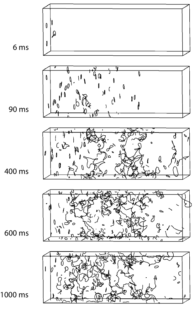
Figure 1: Simulation of quantum turbulence formation. Each frame shows the vortex configuration at the labeled time. Rings injected from the left quickly collide and recombine producing a vortex tangle which evolves on longer timescales.

Our simulation methods Tsubota00 follow those of Schwarz Schwarz85 . A vortex line is represented by a string of points along its core. The problem is greatly simplified at $T$=0 since, with no normal fluid, each point moves with the local superfluid velocity which is calculated by full Biot-Savart integration. (Although the order parameter of superfluid ³He is more complex, the equations which govern superfluid flow of ³He-B in low magnetic fields are identical to those of superfluid ⁴He, except that the vortices in ³He-B have larger, more complex, cores and the circulation quantum is a little smaller vollhardt .) While there is no explicit decay process in the simulations, vorticity is lost in two ways. First, vortices can escape through the open ends of the simulation cell, equivalent to the escape of vorticity beyond the detector range in the experiment. Second, energy is lost when transferred to structures smaller than the numerical space resolution set by the average point spacing on the filament (0.5 $\mu$m in our case). The justification of this cutoff procedure is discussed in detail in ref. Tsubota00 .

At a low injection rate ($\tau_{i}=5$ ms), simulations confirm that the rings travel essentially independently. Their relatively high speed results in a rapid loss of vorticity from the simulation cell when the injection ceases. This corresponds to the rapid decay of the vorticity signal observed in the experiments at low grid velocities gridrings .

At higher ring injection rates, corresponding to higher grid velocities, we see very different behavior as shown in Fig. 1 for $\tau_{i}=1.5$ ms. Here, the rings immediately start to collide and reconnect, establishing a vortex tangle at the center of the box. This corresponds to the behavior observed at high grid velocities in ref. gridrings , namely quantum turbulence which decays on much slower timescales. The simulations are consistent with a sharp transition between the two regimes as observed experimentally.

We now turn to the transient behavior after switching on the ring generation. In Fig. 2 we plot the build-up of the vortex line density (line length per unit volume) after commencing the ring injection. The upper plot shows line-densities obtained in the simulations, averaged over the simulation volume. The highest curve corresponds to the simulation of Fig. 1. At low ring injection rates, the rings propagate independently and fill the simulation volume within the ring transit time $L_{0}/v\sim 0.14$ s. The steady state line density for independent vortex rings is easily calculated. The injected vortex-ring flux along the forward direction is $(A\tau_{i})^{-1}$. Assuming that the rings travel independently and approximately in the forward direction, the equilibrium line density for the rings is

$$L_{ring}\simeq\pi D/(Av\tau_{i}).$$ (1)

This is shown by the horizontal lines in Fig. 2. At higher injection rates the steady-state ring density occurs transiently, followed by a slower increase as the tangle forms.

The lower part of Fig. 2 shows the experimental data for a range of grid velocities. At the lower velocities it takes around a second for the full signal to develop, the initial rise time being limited by the mechanical response time of the grid resonator. At the higher velocities we see a further longer time evolution coinciding with the onset of turbulence. Given the simple assumptions made, the correspondence between simulation and experiment is striking. The line density increases as the tangle forms as this sluggish object acts as an effective trap for incoming rings further increasing the line density. The balance between the ring injection rate and the dissipation (see below) determines the equilibrium line density.

To estimate the timescale for developing the turbulent tangle, we note that the longest timescales are associated with the largest vortex structures which will have sizes approaching that of the turbulent region $\mathcal{L}$. Assuming a Kolmogorov spectrum, the characteristic velocity on a length scale $\mathcal{L}$ is $v(\mathcal{L})\simeq C^{1/2}\epsilon^{1/3}(\mathcal{L}/2\pi)^{1/3}$ where $C\simeq 1.6$ is the Kolmogorov constant and the dissipation per unit mass can be written as $\epsilon=\zeta\kappa^{3}L^{2}$ Vinen , where the dimensionless constant $\zeta\simeq 0.2$ is inferred experimentally from the decay data griddecay . We can then estimate the development timescale as

$$\tau\simeq\frac{\mathcal{L}}{v(\mathcal{L})}\simeq\frac{1}{\sqrt{C}}\left(\frac{2\pi}{\zeta}\right)^{1/3}\frac{1}{\kappa}\left(\frac{\mathcal{L}}{L}\right)^{2/3}.$$ (2)

For the simulations, using $\mathcal{L}\simeq L_{0}=600$ $\mu$m and $L\simeq 6\times 10^{8}$ m^-2 gives $\tau\sim 0.4$ s, and for the experiments with $\mathcal{L}\sim 1$ mm and $L\simeq 1\times 10^{8}$ m^-2 gives $\tau\sim 2$ s, in excellent agreement with the results in Fig. 2.

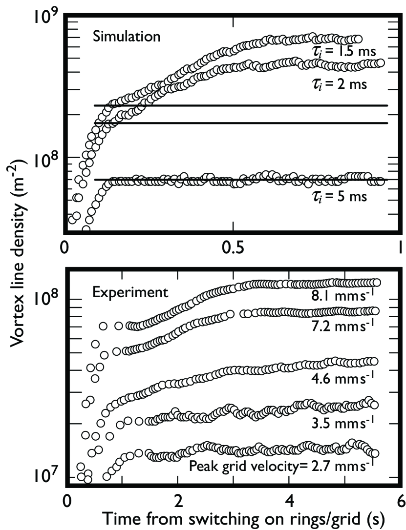
Figure 2: Upper figure: the mean vortex line density from the simulations, for different ring injection-time intervals, steady-state line densities for free rings are indicated by the horizontal lines. Lower figure: the vortex line density as measured for various grid velocities, the tangle forms above $\sim 3.5$ mms^-1.

We may also estimate the critical vortex ring line density for the onset of turbulence. The spread of ring speeds along the forward direction is $\sim v(1-\cos\theta)\sim v\theta^{2}/2$. To collide and reconnect, two rings must approach within a ring diameter, thus the probability of any given ring reconnecting per unit time is $\sim\pi D^{2}\theta^{2}/(2A\tau_{i})$. Multiplying by the cell transit time $\sim L_{0}/v$ and the number of rings $\sim L_{0}/(v\tau_{i})$ gives the total probability of a reconnection event somewhere in the box, $p\sim(\pi/2A)(D\theta L_{0}/\tau_{i}v)^{2}$. Once two rings have reconnected, the larger fragment has a much lower velocity and is thus far more likely to collide with other rings, rapidly leading to a vortex tangle. We may therefore estimate the condition for the onset of turbulence as $p\sim 1$, which gives us a critical ring injection time and a corresponding critical line density

$$L_{c}\sim\frac{1}{L_{0}\theta}\sqrt{\frac{2\pi}{A}}.$$ (3)

This is a lower bound since it assumes that turbulence sets in as soon as any two rings collide, while in fact more collisions may be needed. Applied to the simulation, equation 3 predicts $L_{c}\sim 6\times 10^{7}$ m^-2 whereas the simulations in Fig. 2 show turbulence starting between $L=7\times 10^{7}$ m^-2 and $L=2\times 10^{8}$ m^-2. Comparison with experiment is harder since the critical density will be affected by several other factors such as the complex three dimensional geometry and the distribution of ring sizes and emission angles. However the simple expression gives roughly the correct order of magnitude for the critical line density, with $\theta\sim 10^{\circ}$ and $L_{0}\sim 1$ mm.

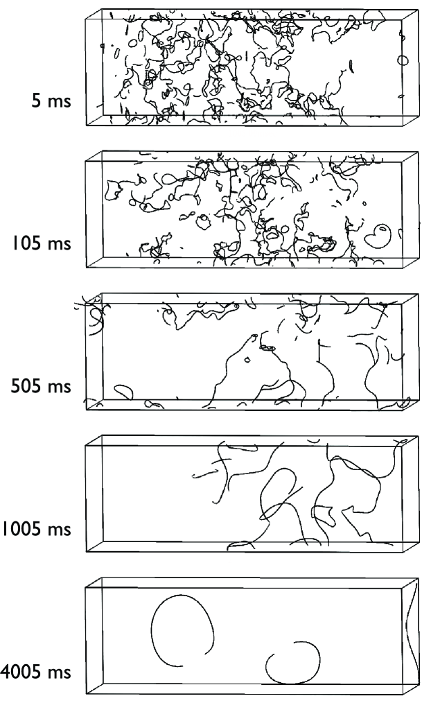
Figure 3: Simulation of the decay of vorticity. The starting configuration is the last frame in Fig. 1. The frame labels indicate the time after cessation of ring injection.

We now discuss the decay of the turbulence. Fig. 3 shows a continuation of the simulation of Fig. 1 after stopping the ring injection. By 0.1 s the loss of the incoming rings leaves a clear volume to the left with a slowly decaying tangle in the center. There is a small loss of vorticity through the ends of the simulation cell but the majority of the loss is into features smaller than the computational space resolution, which effectively gives a length scale below which vorticity is dissipated as assumed in the Richardson cascade of classical turbulence.

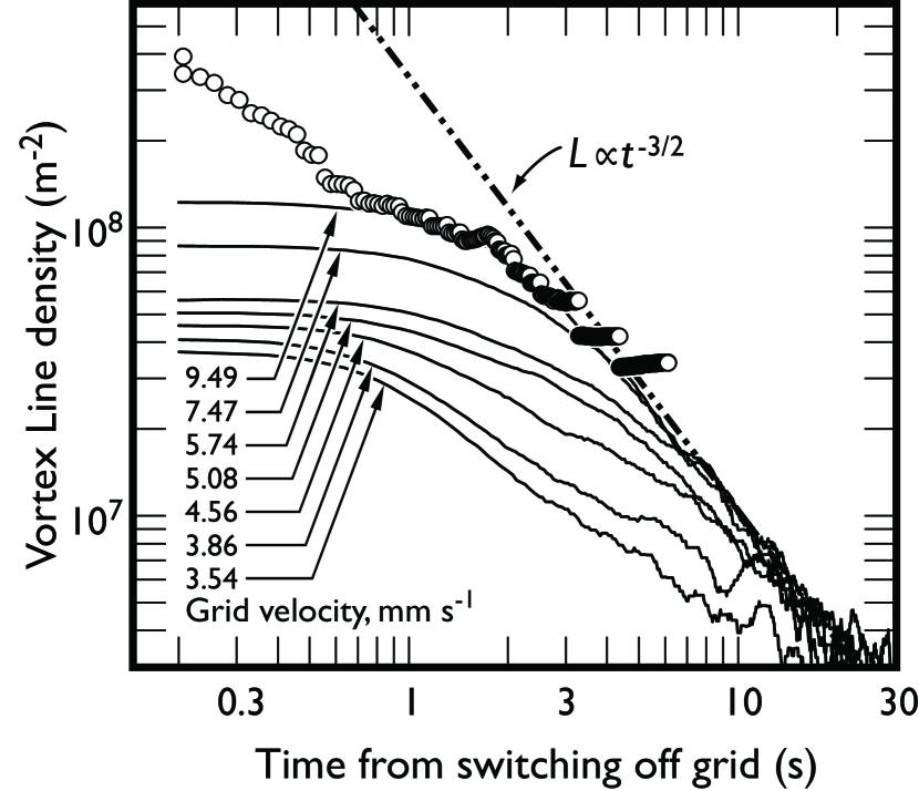
Figure 4: Decay of the vortex line density. Circles show results from the simulation in Fig. 3. Lines show experimental data from ref. griddecay . Dashed line shows the expected late-time limiting behavior for a classical-like Richardson cascade.

In Fig. 4, we compare directly the decay of the line density from the simulation of figure 3 with the experimental measurements at high grid velocities griddecay . The late-time limiting behavior, $L\sim t^{-3/2}$, shown by the dashed line in the figure, provides indirect evidence of a Richardson cascade griddecay , transferring energy from large to small length scales where dissipation ultimately takes place. Similar behavior has been observed in superfluid ⁴He experiments Golov ; Stalp and in earlier simulations TsubotaKolmogorov . While in classical turbulence viscosity provides the decay mechanism, turbulent decay in a superfluid at $T$=0 appears to be governed by the circulation quantum griddecay ; Golov ; Stalp , possibly from radiation by high-frequency Kelvin waves emitted by kinks left by vortex reconnections Svistunov ; Kelvinwaves ; Vinen . At late times the simulated line density runs into problems of the limited simulation volume, however there is a remarkably close similarity to the experimental data. Given that the simulations simply remove energy from small length scales with no overt physical mechanism, the result strongly suggests that, provided dissipation occurs only at small length scales, the late time decay is insensitive to the precise dissipation mechanism.

In conclusion we have demonstrated that for a pure quantum fluid carrying turbulence we now have the computational tools to undertake a full Biot-Savart simulation of the evolution of the vorticity over significant volumes and time scales to make meaningful comparisons with experiments. The agreement with the observed behavior in the present case is quite startling. The particular experiment chosen for this comparison, grid turbulence, exhibits not only a Richardson-type cascade from larger to smaller scale structures but also a reverse cascade from smaller to larger length scales as the initial gas of small precursor vortex loops recombine to form larger and larger structures. The simulations allow a detailed investigation of the various processes involved. Furthermore, the experimental observation of a vortex-ring gas as a precursor to turbulence was completely unexpected but is easily understood in the present simulations. In this paper we are limited to static figures. Many more details, such as the influence of Kelvin waves produced by recombination events, are revealed by studying the full time evolution (the full simulations can be seen as videos at http://matter.sci.osaka-cu.ac.jp/ bsr/tsubotag). We expect that many further interesting results will arise from more detailed analysis. For instance, we have recently been studying fluctuations in the vortex line density which show a Kolmogorov-like, $-5/3$ power law, frequency spectrum as found experimentally gridfluc ; he4fluc . Details will be reported elsewhere.

The ability to apply realistic simulations to experiments represents a significant milestone in the study of quantum turbulence which will greatly enhance our interpretation of experiments and our detailed understanding. We are also learning that quantum turbulence carries a strong resemblance to classical turbulence and may therefore provide new insights into turbulence in general.

We acknowledge technical support from M.G.Ward and A.Stokes, and funding from: the Japanese JSPS; the Japanese MEXT; the UK EPSRC; the FP7 European MicroKelvin network; and the Royal Society.

References

- (1) S.N. Fisher, A.J. Hale, A.M. Guénault and G.R. Pickett, Phys. Rev. Lett. 86, 244 (2001).
- (2) D.I. Bradley, S.N. Fisher, A.M. Guénault, M.R. Lowe, G.R. Pickett, A. Rahm and R.C.V. Whitehead, Phys. Rev. Lett. 93, 235302 (2004).
- (3) D.I. Bradley, D.O. Clubb, S.N. Fisher, A.M. Guénault, R.P. Haley, C.J. Matthews, G.R. Pickett, V. Tsepelin and K. Zaki, Phys. Rev. Lett. 95, 035302 (2005).
- (4) D.I. Bradley, D.O. Clubb, S.N. Fisher, A.M. Guénault, R.P. Haley, C.J. Matthews, G.R. Pickett, V. Tsepelin and K. Zaki, Phys. Rev. Lett. 96, 035301 (2006).
- (5) D.I. Bradley, D.O. Clubb, S.N. Fisher, A.M. Guénault, C.J. Matthews and G.R. Pickett, J. Low Temp. Phys. 134, 381 (2004).
- (6) D.I. Bradley, S.N. Fisher, A.M. Guénault, R.P. Haley, S. O Sullivan, G.R. Pickett and V. Tsepelin, Phys. Rev. Lett. 101 065302 (2008).
- (7) D.I. Bradley, S.N. Fisher, A.M. Guénault, R.P. Haley, M. Holmes, S. O Sullivan, G.R. Pickett and V. Tsepelin, J. Low Temp. Phys. 150, 364 (2008).
- (8) R. Hänninen, A. Mitani, and M. Tsubota, AIP Conf. Proc. 850, 217 (2006).
- (9) D.I. Bradley, S.N. Fisher, A.M. Guénault, R.P. Haley, C.J. Matthews, G.R. Pickett, J. Roberts, S. O Sullivan and V. Tsepelin, J. Low Temp. Phys. 148, 235 (2007).
- (10) K.W. Schwarz, Phys. Rev. B 31, 5782 (1985).
- (11) J. Koplik and H. Levine, Phys. Rev. Lett. 71, 1375 (1993).
- (12) M. Tsubota, T. Araki and S.K. Nemirovskii, Phys. Rev. B 62, 11751 (2000).
- (13) D. Vollhardt,P. Wölfle The Superfluid phases of Helium 3 (Taylor & Francis), (1990).
- (14) W.F. Vinen and J.J. Niemela, J. Low Temp. Phys. 128, 167 (2002).
- (15) P.M. Walmsley, A.I. Golov, H.E. Hall, A.A. Levchenko and W.F. Vinen, Phys. Rev. Lett. 99, 265302 (2007).
- (16) S.R. Stalp, L. Skrbek and R.J. Donnelly, Phys. Rev. Lett. 82, 4831 (1999).
- (17) T. Araki, M. Tsubota and S.K. Nemirovskii, Phys. Rev. Lett. 89, 145301 (2002).
- (18) B.V. Svistunov, Phys. Rev. B 52, 3647 (1995).
- (19) D. Kivotides, J.C. Vassilicos, D.C. Samuels and C.F. Barenghi, Phys. Rev. Lett. 86, 3080 (2001).
- (20) P.E. Roche, P. Diribarne, T. Didelot, O. Francais, L. Rousseau and H. Willaime, Europhys. Lett. 77, 66002 (2007).