The Best Linear Unbiased Estimator for Continuation of a Function

Abstract

We show how to construct the best linear unbiased predictor (BLUP) for the continuation of a curve in a spline-function model. We assume that the entire curve is drawn from some smooth random process and that the curve is given up to some cut point. We demonstrate how to compute the BLUP efficiently. Confidence bands for the BLUP are discussed. Finally, we apply the proposed BLUP to real-world call center data. Specifically, we forecast the continuation of both the call arrival counts and the workload process at the call center of a commercial bank.

tablecaptionshape tablename skip. 

, and

1 Introduction

Many data sets consist of a finite number of multidimensional observations, where each of these observations is sampled from some underlying smoothed curve. In such cases it can be advantageous to address the observations as functional data rather than as multiple series of data points. This approach was found useful, for example, in noise reduction, missing data handling, and in producing robust estimations (see the books Ramsay and Silverman, 2002; Ramsay and Silverman, 2005, for a comprehensive treatment of functional data analysis). In this work we consider the problem of forecasting the continuation of a curve using functional data techniques.

The problem we consider here is relevant to longitudinal data sets, in which each observation consists of a series of measurements over time that describe an underlying curve. Examples of such curves are growth curves of different individuals and arrival rates of calls to a call center or of patients to an emergency room during different days. We assume that such curves, or measurement series that approximate these curves, were collected previously. We would like to estimate the continuation of a new curve given its beginning, using the behavior of the previously collected curves.

Although each observation consists of a finite number of points, the observation can be thought of as a smooth function. This dual representation leads to two different approaches when attempting to solve the prediction problem. In the discrete approach, each observation is a longitudinal vector of length $p+q$. We are interested in the prediction of the last $q$-length part of the new observation, given its beginning $p$-length part. This can be computed by treating the beginning $p$-length vector as the predictor variables and the last $q$-length vector as the response variables. A prediction can be found, for example, by finding the best linear unbiased predictor (see (5)). The disadvantage of the discrete approach is that the smooth nature of the underlying function is ignored. If, instead, the continuous approach is used, the prediction problem might be treated naively using regression techniques in which both the predictor and the response are functions (Ramsay and Silverman, 2005, Chapter 16). However, these techniques do not take into account the fact that the response function is a smooth continuation of the predictor function.

In this paper, we choose the continuous approach. Specifically, we would like to generalize the discrete case to the continuous one, taking the smooth nature of the curves into account. There are three main points that need to be addressed. First, the curves lie within an infinite dimensional space, while the number of observed curves is finite. This indicates that a simple model for description of the data is required. Second, the full-length curves, the curve beginnings, and the curve continuations all lie in different functional spaces, which, in contrast to the discrete case, cannot generally be related by a linear projection. Third, we require that the prediction should be a smooth continuation of the beginning of the curve (at least in the absence of noise).

Forecasting of the continuation of a function was considered in previous works. Besse, Cardot and Stephenson (2000), and Antoniadis, Paparoditis and Sapatinas (2006), among others, developed different techniques for curve-valued autoregressive processes. In these models, each curve describes some longitudinal data cycle such as climate variation during a year (Besse, Cardot and Stephenson, 2000) and television audience rates during a day (Antoniadis, Paparoditis and Sapatinas, 2006). These models assume that the cycles behave according to some autoregressive model. The aim of these works is to predict the next cycles given past observed cycles. The continuity point at the beginning of each cycle, if it exists, is usually not taken into account. The model discussed in Shen (2009) is closer to ours. Shen discusses a curved-valued time series model in which past curves were previously observed, and the beginning part of a new curve is given. Shen first forecasts the new curve entirely, and then updates this forecast based on the given curve beginning using penalized least squares. However, all the models discussed above assume some time series behavior, while the model discussed here assumes that the curve-valued observations are independent.

The forecasting of curve continuation suggested here is based on finding the best linear unbiased predictor (BLUP) (Robinson, 1991). We assume that the curves are governed by a small number of factors, possibly with additional noise. These factors determine the main variation between the different curves. The computation of the predictor is performed in two steps. First, the factors’ coefficients are estimated from the beginning of the new curve, which is defined on the first part of the segment. Second, the prediction is obtained by computing the representation of the factors on the latter part of the segment. We prove that the resulting estimator is indeed the BLUP and that it is a smooth continuation of the beginning of the curve (at least in the absence of noise).

The two-step procedure for obtaining the BLUP involves computation of the mean function on both partial segments, and of the covariance operator on both segments and between them, which can be computationally demanding if not performed prudently. We approximate the curve data using a spline function space of (possibly large) finite-dimension (de Boor, 2001). More specifically, we represent the curves using appropriate B-splines bases. The use of splines is common in functional data analysis due to the simplicity of spline computation, and the ability of splines to approximate smooth functions. We take advantage of two more attributes of finite-dimensional spline functional spaces. First, the functional space restriction from the whole segment to a partial segment (the beginning part or the latter part) has a natural B-spline basis that has a lower number of elements. This solves collinearity problems which can render any projection on the partial segment basis instable. Second, the knot-insertion algorithm (see de Boor, 2001, Chapter 11) ensures an efficient and stable way to compute the mean function and covariance operators on different partial segments.

The proposed forecasting procedure yields a smooth curve which is the best linear unbiased prediction. Note, however, that the continuation part of the function is random, and therefore requires confidence bands. We present confidence bands for the prediction, following Knafl, Sacks and Ylvisaker (1985), under the assumption that the curves aries from a Gaussian process. The bands are computed in two steps. First, confidence intervals are computed simultaneously for a finite set of points. Then, using the fact that splines are piecewise polynomials, a global band is found. We also suggest a way to compute confidence bands using cross-validation. While no theoretical justification proof is given for the cross validation confidence bands, they are much faster to compute, and the numerical examples in Section 5 show that this approach works considerably well.

We apply the forecasting procedure suggested here to call center data. We forecast the continuation of two processes: the arrival process and the workload process (i.e., the amount of work in the system; see, for example, Aldor-Noiman, Feigin and Mandelbaum, 2009). In call centers, the forecast of the arrival process plays an important roll in determining staffing levels. Optimization of the latter is important since salaries account for about 60-70% of the cost of running a call center (Gans, Koole and Mandelbaum, 2003). Usually, call center managers utilize forecasts of the arrival process and knowledge of service times, along with some understanding of customer patience characteristics (Zeltyn, 2005), to estimate future workload and determine staffing level (Aldor-Noiman, Feigin and Mandelbaum, 2009). The disadvantage of this approach is that the forecast of the workload is not performed directly, and instead it is obtained using the forecast of the arrival process. Reich (2010) showed how the workload process can be estimated explicitly, thereby enabling direct forecast of the workload. In this work we forecast the continuation of both the arrival and workload processes, given past days’ information and the information up to some time of the day. We compare between the results for the arrival process and the workload process. We also compare our results for the arrival process to those of other forecasting techniques, namely, to the techniques that were introduced by Weinberg, Brown and Stroud (2007) and Shen and Huang (2008).

The paper is organized as follows. The functional model and notation are presented in Section 2. The main theoretical results are presented in Section 3, were we first show how to construct the BLUP for the continuation of a curve. Next, we show how the BLUP can be computed efficiently. Confidence bands are discussed in Section 4. In Section 5 we apply the estimator to real-world data, comparing direct and indirect workload forecasting, and comparing our results to other techniques. Concluding remarks appear in Section 6. Technical proofs are provided in the Appendix.

2 The functional model

In this section we present the model and notation that will be used throughout this paper. Let $X$ be a random function defined on the segment $S=[0,T]$, and let the random functions $X_{1}$ and $X_{2}$ be the restrictions of $X$ to the segments $S_{1}=[0,U]$ and $S_{2}=[U,T]$, respectively, for some $0<U<T$. Our goal is to estimate $X_{2}$ given information regarding $X_{1}$.

We assume that $X$ is of the form

$$X(t)=\mu(t)+\bm{\phi}(t)^{\prime}\bm{h}\,,$$

where $\mu(t)$ is the mean function, $\bm{h}=(h_{1},\ldots,h_{p})$ is a random vector with mean zero and covariance matrix $L$, $L$ is diagonal with $L_{11}\geq\ldots\geq L_{pp}>0$, and $\bm{\phi}(t)=(\phi_{1}(t),\ldots,\phi_{p}(t))^{\prime}$ is a vector of orthonormal functions. We assume that the functions $\mu$ and $\phi_{j}$ have a basis expansion with respect to some B-spline basis $\bm{b}=(b_{1},...,b_{N})^{\prime}$, defined on some fixed knot sequence $\tau$. We denote this B-spline space by $S_{k,\tau}$ where $k$ denotes the the splines’ order. Thus, we can write $\mu(t)=\bm{b}(t)^{\prime}\bm{\mu}$ and $\bm{\phi}(t)=A^{\prime}\bm{b}(t)$, for some $p\times 1$ vector $\bm{\mu}$ and $N\times p$ loading matrix $A$. Thus, we have

$$X(t)=\bm{b}(t)^{\prime}\big{(}\bm{\mu}+A\bm{h}\big{)}\doteq\bm{b}(t)^{\prime}\bm{x}\,,$$ (1)

where $\bm{x}=\bm{\mu}+A\bm{h}$. We think of $N$, the ambient functional space dimension, as being much larger then $p$, the dimension of the subspace which spanned by the random function $X$.

We assume that instead of seeing $X$, we actually observe some noisy version of $X$, namely

$$Y(t)=X(t)+\varepsilon(t)\,,$$

where $\varepsilon(t)=\bm{\psi}(t)^{\prime}\bm{\epsilon}$ is some random function independent of $X(t)$, $\bm{\epsilon}$ is a $q\times 1$ zero-mean random vector with diagonal covariance matrix $\Sigma$, and $\bm{\psi}$ is a vector of functions. Since $X(t)$ is a (random) linear combination of $\phi_{1}(t),\ldots,\phi_{p}(t)$, we consider the noise as the part of the observed function $Y(t)$ that cannot be explained using such linear combinations. Hence we assume that $\bm{\psi}$ is orthogonal to $\bm{\phi}$. However, note that this orthogonality is not necessarily preserved when $\bm{\psi}$ and $\bm{\phi}$ are restricted to one of the segments $S_{1}$ or $S_{2}$. We assume that $\bm{\psi}$ also has an expansion with respect to the basis $\bm{b}$ and hence $\bm{\psi}(t)=B^{\prime}\bm{b}(t)$ for some $N\times q$ loading matrix $B$. Using this notation we may write

$$Y(t)=\bm{b}(t)^{\prime}\big{(}\bm{\mu}+A\bm{h}+B\bm{\epsilon}\big{)}\,.$$ (2)

The covariance functions $u(s,t)=\textrm{Cov}(X(s),X(t))$ and $v(s,t)=\textrm{Cov}(Y(s),Y(t))$ can be written by $\bm{b}(s)^{\prime}(ALA^{\prime})\bm{b}(t)\doteq\bm{b}(s)^{\prime}g\bm{b}(t)$ and $\bm{b}(s)^{\prime}(ALA^{\prime}+B\Sigma B^{\prime})\bm{b}(t)\doteq\bm{b}(s)^{\prime}G\bm{b}(t)$, respectively. We define the correspondence covariance operators from $S_{k,\tau}$ to itself for functions $f\in S_{k,\tau}$ as

$$(\gamma f)(t) = \int_{S}u(s,t)f(s)\mathrm{d}s=\bm{b}(t)^{\prime}gW\bm{f}$$

$$(\Gamma f)(t) = \int_{S}v(s,t)f(s)\mathrm{d}s=\bm{b}(t)^{\prime}GW\bm{f}$$

where $W=\int_{S}\bm{b}(s)\bm{b}(s)^{\prime}\mathrm{d}s$, and $\bm{f}$ is the expansion of the function $f$ in the B-spline basis.

We now introduce the notation for $X_{1}$ and $X_{2}$ and their respective noisy versions $Y_{1}$ and $Y_{2}$. Let $\tau_{1}$ and $\tau_{2}$ be knot sequences that agree with $\tau$ on the segments $[0,U)$ and $(U,T]$, respectively, and have knot multiplicity of $k$ at $U$. Let $S_{k,\tau_{i}}$ for $i=1,2$ be the $k$-ordered spline space with knot sequence $\tau_{i}$ and let $\bm{b}_{\bm{i}}(t)=(b_{i1}(t),\ldots,b_{iN_{i}}(t))$ be its corresponding B-spline basis. We wish to represent $X_{i}$ and $Y_{i}$ ($i=1,2$) using the representations of $X$ and $Y$.

Note that when the functions $\mu(t)$, $\phi_{j}(t)$, $\psi_{j}(t)$, $v(s,t)$ and $u(s,t)$ are known on $[0,T]$, they are also known on $S_{1}$ and $S_{2}$. Thus, it is enough to represent these functions using the bases $\bm{b}_{\bm{i}}$ in order to obtain representations for $X_{i}$ and $Y_{i}$. Recall that $\mu(t)=\bm{b}(t)^{\prime}\bm{\mu}$ for some vector of coefficients $\bm{\mu}$. Using the knot-insertion algorithm (see de Boor, 2001, Chapter 11) we obtain new vectors $\bm{\mu}_{\bm{i}}$ such that (a) $\mu(t)=\bm{b}_{\bm{i}}(t)^{\prime}\bm{\mu}_{\bm{i}}$ for all $t$ on which $\bm{b}_{\bm{i}}$ is defined and (b) $\bm{\mu}_{\bm{i}}$ is obtained from $\bm{\mu}$ by truncation and a change of at most $k$ coefficients. Similarly, using the knot-insertion algorithm, we can obtain the loading matrices $A_{i}$ and $B_{i}$ such that $\bm{\phi}(t)=A_{i}\bm{b}_{\bm{i}}(t)$ and $\bm{\psi}(t)=B_{i}\bm{b}_{\bm{i}}(t)$ for all $t$ on which $\bm{b}_{\bm{i}}$ is defined. Summarizing, we have

$$X_{i}(s) = \bm{b}_{\bm{i}}(s)^{\prime}\big{(}\bm{\mu}_{\bm{i}}+A_{i}\bm{h}\big{)}\doteq\ \bm{b}_{\bm{i}}(s)^{\prime}\bm{x}_{\bm{i}}$$ (3)

$$Y_{i}(s) = \bm{b}_{\bm{i}}(s)^{\prime}\big{(}\bm{\mu}_{\bm{i}}+A_{i}\bm{h}+B_{i}\bm{\epsilon}\big{)}\doteq\bm{b}_{\bm{i}}(s)^{\prime}\bm{y}_{\bm{i}}$$

$$v(s,t) = \bm{b}_{\bm{i}}(s)(A_{i}LA_{j}^{\prime}+B_{i}\Sigma B_{j}^{\prime})\bm{b}_{\bm{j}}(t)\doteq\bm{b}_{\bm{i}}(s)^{\prime}G_{ij}\bm{b}_{\bm{j}}(t)$$

$$u(s,t) = \bm{b}_{\bm{i}}(s)(A_{i}LA_{j}^{\prime})\bm{b}_{\bm{j}}(t)\doteq\bm{b}_{\bm{i}}(s)^{\prime}g_{ij}\bm{b}_{\bm{j}}(t)$$

for $i,j=1,2$ and for each $s\in S_{i}$ and $t\in S_{j}$.

We define the operators $\gamma_{ij}$ and $\Gamma_{ij}$ from $S_{k,\tau_{j}}$ to $S_{k,\tau_{i}}$ for $i,j=1,2$ by

$$(\gamma_{ij}f)(t) = \int_{S_{j}}u(s,t)f(s)\mathrm{d}s=\bm{b}_{\bm{i}}(t)^{\prime}g_{ij}W_{j}\bm{f}$$ (4)

$$(\Gamma_{ij}f)(t) = \int_{S_{j}}v(s,t)f(s)\mathrm{d}s=\bm{b}_{\bm{i}}(t)^{\prime}G_{ij}W_{j}\bm{f}\,,$$

where $W_{j}=\int_{S_{j}}\bm{b}_{\bm{j}}(s)\bm{b}_{\bm{j}}(s)^{\prime}\mathrm{d}s$, and $\bm{f}$ is the expansion of the function $f$ in $\bm{b}_{\bm{j}}$.

The model discussed above will be used for the estimation of $X_{2}$ given $Y_{1}$. Note that the distributions of $X$ and $Y$ are generally not known. In a realistic situation one needs to estimate the model components. Recall that $Y(t)=\bm{b}(t)^{\prime}\big{(}\bm{\mu}+A\bm{h}+B\bm{\epsilon}\big{)}$, where $\bm{h}$ and $\bm{\epsilon}$ are random vectors with zero mean and covariance matrices $L$ and $\Sigma$, respectively. Before discussing the forecasting procedure, we briefly discuss how estimation of $\bm{\mu},L,\Sigma$ and the loading matrices $A$ and $B$ can be performed.

Assume that the functions $Y^{(1)},\ldots,Y^{(m)}$ were drawn according to the distribution law of $Y$. We distinguish between two scenarios. In the first scenario we assume that the functions $Y^{(1)},\ldots,Y^{(m)}$ were observed. In this case one can estimate the various components of $Y$ using functional principal component analysis (functional PCA). This can be done either by using PCA on the coefficients of the functions or by introducing some smoothness using regularized functional PCA (see, for example, Ramsay and Silverman, 2005, Chapters 8 and 9). The matrices $L$ and $\Sigma$ are then determined by the eigenvalues of the PCA decomposition while the loading matrices $A$ and $B$ consist of the coefficients of the principal components with respect to the basis $\bm{b}$. The size of $L$ and $\Sigma$ can be estimated using the gaps in the eigenvalues of the PCA decomposition.

In the second scenario, we assume that some noisy discrete observations are given; for example in the following form

$$Z^{(i)}(t_{ij})=Y^{(i)}(t_{ij})+e_{ij}\,,$$

for $i=1,\ldots,m$, $j=1,\ldots,n_{j}$, and $0\leq t_{i1}<\ldots<t_{in_{j}}\leq T$, and where $e_{ij}\sim N(0,\sigma^{2})$ are independent. In this case, one can first estimate the functions and then use functional PCA as described above. The simplest way to estimate the functions is to estimate each function separately, using, for example, regression splines (de Boor, 2001, Chapter 14). This method is used in the numerical examples in Section 5. Others, such as Kneip (1994) and Besse, Cardot and Ferraty (1997), suggest to estimate all the functions simultaneously. Both methods use some sort of functional PCA. These methods suggest ways to estimate the length of $\bm{h}$. The method by Besse, Cardot and Ferraty (1997) also assumes a splines environment, as in our case.

3 The construction of the BLUP

Given $Y_{1}$, the noisy version of the beginning part of the random function $X$, our goal is to find a good estimator for $X_{2}$, the continuation of $X_{1}$.

Following Robinson (1991), we say that $\hat{X}_{2}$ is a good estimator of $X_{2}$ given $Y_{1}$ if the following criteria hold:

1. $\hat{X}_{2}$ is a linear function of $Y_{1}$.

2. $\hat{X}_{2}$ is unbiased, i.e., $E[\hat{X}_{2}(t)]=\mu(t)$.

3. $\hat{X}_{2}$ has minimum mean square error among the class of linear unbiased estimators.

Two more demands regarding the estimator that seems desirable in our context are

1. The random function $\hat{X}_{2}$ lies in the space $S_{k,\tau_{2}}$.

2. When no noise is introduced, i.e., when $Y_{1}=X_{1}$, the concatenation of $\hat{X}_{2}$ to $X_{1}$ lies in $S_{k,\tau}$; in other words, the combined function

   $$\hat{X}=\left\{\begin{array}[]{cc}X_{1}(t)&0\leq t\leq U\\ \hat{X}_{2}(t)&U<t\leq T\\ \end{array}\right.$$

   is smooth enough.

An estimator that fulfills (C1)-(C5) will be referred to as a best linear unbiased predictor (BLUP). In this section we will show how to construct such a BLUP and prove that is is defined uniquely.

Remark 3.1.

Note that the definition of unbiased estimator in (C2) is not the usual definition. A more restrictive criterion is

1. $\hat{X}_{2}$ is unbiased in the the following sense $E[\hat{X}_{2}(t)|Y_{1}]=E[X_{2}(t)|Y_{1}]$.

We will show that when $Y$ is a Gaussian process, this criterion is fulfilled by the proposed BLUP as well.

Remark 3.2.

The analogous results in the multivariate case are well known. Here best estimator means estimator that meets criteria (C1)-(C3). Let $Z=(Z_{1},Z_{2})^{\prime}$ be a random vector such that

$$E\left[\begin{array}[]{c}Z_{1}\\ Z_{2}\\ \end{array}\right]=\left(\begin{array}[]{c}m_{1}\\ m_{2}\\ \end{array}\right)\,,\quad\mathrm{Var}\left[\begin{array}[]{c}Z_{1}\\ Z_{2}\\ \end{array}\right]=R=\left(\begin{array}[]{cc}R_{11}&R_{12}\\ R_{21}&R_{22}\\ \end{array}\right)\,.$$

Then the BLUP of $Z_{2}|Z_{1}$ is given by

$$\hat{Z}_{2}=m_{2}+R_{21}R_{11}^{+}(Z_{1}-m_{1})$$ (5)

where $R_{11}^{+}$ is the Moore-Penrose pseudoinverse of $R_{11}$ (see, for example, Marsaglia, 1964).

In the following, we define the linear operators that are the analogs of the matrices $R_{11}^{+}$ and $R_{21}$ from the multivariate case. This enables the construction of a uniquely-defined BLUP for $X_{2}$.

We begin with defining the operator $\Gamma_{11}^{+}:S_{k,\tau_{1}}\rightarrow S_{k,\tau_{1}}$, which is the functional equivalent of $R_{11}^{+}$. Define the function

$$v_{11}^{+}(s,t)=\bm{b}_{\bm{1}}(s)^{\prime}W_{1}^{-1}G_{11}^{+}W_{1}^{-1}\bm{b}_{\bm{1}}(t)\,,$$

for every $s,t\in S_{1}$. Note that $W_{1}$ is invertible since it is a Gram matrix of basis functions (see Sansone, 1991, Theorem 1.5). Define

$$(\Gamma_{11}^{+}f)(t)=\int_{S_{1}}v_{11}^{+}(s,t)f(s)\mathrm{d}s=\bm{b}_{\bm{1}}(t)^{\prime}W_{1}^{-1}G_{11}^{+}\bm{f}\,,$$

where $\bm{f}$ is the expansion of the function $f$ in the B-spline basis $\bm{b}_{\bm{1}}$. The following lemma justifies the notation of $\Gamma_{11}^{+}$ as a pseudoinverse operator.

Lemma 3.3.

With probability one,

$$\Gamma_{11}\Gamma_{11}^{+}(Y_{1}-\mu)=\Gamma_{11}^{+}\Gamma_{11}(Y_{1}-\mu)=Y_{1}-\mu\,.$$

See proof in the Appendix.

We are now ready to define the estimator for $X_{2}$ given $Y_{1}$, similarly to estimator (5) in the multivariate case, by

$$\hat{X}_{2}(t)=\mu(t)+\gamma_{21}\Gamma_{11}^{+}(Y_{1}-\mu)(t)=\bm{b}_{\bm{2}}(t)^{\prime}\big{(}\bm{\mu}_{\bm{2}}+g_{21}G_{11}^{+}(\bm{y}_{\bm{1}}-\bm{\mu}_{\bm{1}})\big{)}\,,$$ (6)

for every $t\in S_{2}$. Then we have

Theorem 3.4.

The estimator $\hat{X}_{2}$ meets criteria (C1)-(C5) and is unique up to equivalence. Moreover, if $Y$ is a Gaussian process, then $\hat{X}_{2}$ meets criterion (C2*) as well.

Proof.

We show that (C1)-(C5) hold, one by one.

(C1) holds because $\hat{X}_{2}$ is indeed a linear transformation of $Y_{1}$ as can be seen from (6).

(C2) holds since

$$E[\hat{X}_{2}(t)]=\bm{b}_{\bm{2}}(t)^{\prime}\big{(}\bm{\mu}_{\bm{2}}+g_{21}G_{11}^{+}(E[\bm{y}_{\bm{1}}-\bm{\mu}_{\bm{1}}])\big{)}=\bm{b}_{\bm{2}}(t)^{\prime}\bm{\mu}_{\bm{2}}=\mu(t)\,.$$

(C3) states that $\hat{X}_{2}$ should minimize the mean square error among all the unbiased linear estimators . Let $\tilde{X}_{2}$ be another linear unbiased estimator. Then we can write $\tilde{X}_{2}=(\tilde{X}_{2}-\hat{X}_{2})+\hat{X}_{2}$. Since both $\tilde{X}_{2}$ and $\hat{X}_{2}$ are unbiased, $\tilde{X}_{2}-\hat{X}_{2}$ is an unbiased linear estimator of zero, hence it is of the form $\bm{b}_{\bm{2}}(t)^{\prime}M(\bm{y}_{\bm{1}}-\bm{\mu}_{\bm{1}})$ for some $N_{2}\times N_{1}$ matrix $M$. Moreover, it can be shown that $\textrm{Cov}(X_{2}-\hat{X}_{2},\tilde{X}_{2}-\hat{X}_{2})=0$. Indeed,

$$\textrm{Cov}\big{(}(X_{2}-\hat{X}_{2})(s),(\tilde{X}_{2}-\hat{X}_{2})(t)\big{)} = E[(X_{2}-\hat{X}_{2})(\tilde{X}_{2}-\hat{X}_{2})(t)]$$

$$= \bm{b}_{\bm{2}}(s)^{\prime}E[(\bm{x}_{\bm{2}}-\bm{\mu}_{\bm{2}})(\bm{y}_{\bm{1}}-\bm{\mu}_{\bm{1}})^{\prime}]M^{\prime}\bm{b}_{\bm{2}}(t)$$

$$\;-\bm{b}_{\bm{2}}(s)^{\prime}E[\bm{\mu}_{\bm{2}}+g_{21}G_{11}^{+}(\bm{y}_{\bm{1}}-\bm{\mu}_{\bm{1}})(\bm{y}_{\bm{1}}-\bm{\mu}_{\bm{1}})^{\prime}]M^{\prime}\bm{b}_{\bm{2}}(t)$$

$$= \bm{b}_{\bm{2}}(s)^{\prime}\big{(}g_{21}M^{\prime}+g_{21}G_{11}^{+}G_{11}M^{\prime})\big{)}\bm{b}_{\bm{2}}(t)=0\,.$$

where the last equality follows from Lemma 3.3.

To see that $\hat{X}_{2}$ minimizes the mean square error, note that

$$E[(X_{2}-\tilde{X}_{2})^{2}(t)] = E[(X_{2}-\hat{X}_{2})^{2}(t)]+E[(\tilde{X}_{2}-\hat{X}_{2})^{2}(t)]+2E[(X_{2}-\hat{X}_{2})(\hat{X}_{2}-\tilde{X}_{2})(t)]$$ (7)

$$= E[(X_{2}-\hat{X}_{2})^{2}(t)]+E[(\tilde{X}_{2}-\hat{X}_{2})^{2}(t)]\geq E[(X_{2}-\hat{X}_{2})^{2}(t)]\,,$$

which proves that $\hat{X}_{2}$ minimizes the mean square error and is unique up to equivalence.

(C4) holds by construction.

(C5) states that when no noise is introduced, $\hat{X}_{2}$ a smooth continuation of $X_{1}$. First, note that by Lemma 3.3

$$X_{1}(t)=\bm{b}_{\bm{1}}(t)^{\prime}\big{(}\bm{\mu}_{\bm{1}}+G_{11}G_{11}^{+}(\bm{x}_{\bm{1}}-\bm{\mu}_{\bm{1}})\big{)}=\bm{b}_{\bm{1}}(t)^{\prime}\big{(}\bm{\mu}_{\bm{1}}+A_{1}(LA_{1}^{\prime}G_{11}^{+})(\bm{x}_{\bm{1}}-\bm{\mu}_{\bm{1}})\big{)}\,.$$

By definition we also have

$$\hat{X}_{2}(t)=\bm{b}_{\bm{2}}(t)^{\prime}\big{(}\bm{\mu}_{\bm{2}}+g_{21}G_{11}^{+}(\bm{x}_{\bm{1}}-\bm{\mu}_{\bm{1}})\big{)}=\bm{b}_{\bm{2}}(t)^{\prime}\big{(}\bm{\mu}_{\bm{2}}+A_{2}(LA_{1}^{\prime}G_{11}^{+})(\bm{x}_{\bm{1}}-\bm{\mu}_{\bm{1}})\big{)}\,.$$

Define $\hat{X}(t)=\bm{b}(t)^{\prime}\big{(}\mu(t)+A(LA_{1}^{\prime}G_{11}^{+})(\bm{x}_{\bm{1}}-\bm{\mu}_{\bm{1}})\big{)}$. It follows from the definitions of $\bm{\mu}_{\bm{i}},A_{i}$ and $\bm{b}_{\bm{i}}$ that $\hat{X}(t)$ agrees with $X_{1}$ on $S_{1}$ and with $\hat{X}_{2}$ on $S_{2}$. Since $\hat{X}\in S_{k,\tau}$, the result follows.

Finally, if $Y$ is a Gaussian process, then $\bm{y}_{\bm{1}}$ and $\bm{x}_{\bm{2}}$ are normally distributed such that $\textrm{Var}(\bm{y}_{\bm{1}})=G_{11}$ and $\textrm{Cov}(\bm{x}_{\bm{2}},\bm{y}_{\bm{1}})=g_{21}$. Following Marsaglia (1964) we obtain

$$E[X_{2}(t)|Y_{1}] = \bm{b}(t)^{\prime}E[\bm{x}_{\bm{2}}|\bm{y}_{\bm{1}}]=\bm{b}(t)^{\prime}\big{(}\bm{\mu}_{\bm{2}}+g_{21}G_{11}^{+}(\bm{y}_{\bm{1}}-\bm{\mu}_{\bm{1}})\big{)}$$

$$= \hat{X}_{2}(t)=E[\hat{X}_{2}(t)|Y_{1}]$$

and criterion (C2*) is met. ∎

It should be noted that when the parameters of the model are estimated (see end of Section 2) and a Gaussian model is assumed, the estimator $\hat{X}_{2}$ can be considered as an empirical Bayes estimator. Indeed, the estimation of the distribution of $\bm{h}$ and $\bm{\epsilon}$ can be considered as estimating the prior distribution, while the the computation of $\hat{X}_{2}$ as in (3) is in fact finding the posterior mean given the data $Y_{1}$.

From a computational point of view, the computation of $\hat{X}_{2}$ may seem heavy. Indeed by (6) it involves finding the pseudoinverse of $G^{+}_{11}$ which is an $N_{1}\times N_{1}$ matrix. However, a simpler expression can be found. Recall that

$$G_{11}=[A_{1},B_{1}]\left[\begin{array}[]{cc}L&0\\ 0&\Sigma\end{array}\right]\left[\begin{array}[]{c}A_{1}^{\prime}\\ B_{1}^{\prime}\\ \end{array}\right]\doteq CSC^{\prime}\,.$$

where $C=[A_{1},B_{1}]$ and $S=\left[\begin{array}[]{cc}L&0\\ 0&\Sigma\end{array}\right]$. Using Lemma A.1.3 with $T=S^{1/2}C^{\prime}$ we have

$$G_{11}^{+} = CS^{1/2}\left(\left(S^{1/2}C^{\prime}CS^{1/2}\right)^{+}\right)^{2}S^{1/2}C^{\prime}$$

$$= CS^{1/2}\left(S^{-1/2}(C^{\prime}C)^{+}S^{-1}(C^{\prime}C)^{+}S^{-1/2}\right)S^{1/2}C^{\prime}$$

$$= C(C^{\prime}C)^{+}S^{-1}(C^{\prime}C)^{+}C^{\prime}\,,$$

which involves the pseudoinverse computation of a $(p+q)\times(p+q)$ matrix.

Finally, instead of assuming that $Y_{1}(t)=\bm{b}_{\bm{1}}(t)^{\prime}\big{(}\bm{\mu}_{\bm{1}}+A_{1}\bm{h}+B_{1}\bm{\epsilon}\big{)}$, one may assume that

$$Y_{1}(t)=\bm{b}_{\bm{1}}(t)^{\prime}\big{(}\bm{\mu}_{\bm{1}}+A_{1}\bm{h}+\bm{\tilde{\varepsilon}}_{\bm{1}}\big{)}$$

where $\bm{\tilde{\varepsilon}}_{\bm{1}}$ is a $N_{1}\times 1$ mean zero random vector with $\sigma^{2}I$ covariance matrix and $I$ is the identity matrix. In this case,

$$\hat{X}_{2}(t)=\bm{b}_{\bm{2}}(t)^{\prime}\big{(}\bm{\mu}_{\bm{2}}+g_{21}(A_{1}LA_{1}^{\prime}+\sigma^{2}I)^{-1}(\bm{x}_{\bm{1}}-\bm{\mu}_{\bm{1}})\big{)}$$ (9)

which is the ridge regression estimator (Hoerl and Kennard, 1970). Once again, a simpler expression can be obtained using some matrix algebra (see Robinson, 1991, Eq. 5.2). We have

$$g_{21}(A_{1}LA_{1}^{\prime}+\sigma^{2}I)^{-1}=A_{2}LA_{1}^{\prime}(A_{1}LA_{1}^{\prime}+\sigma^{2}I)^{-1}=A_{2}\left(A_{1}^{\prime}A_{1}+\sigma^{2}L^{-1}\right)^{-1}A_{1}^{\prime}\,,$$

and hence $\hat{X}_{2}(t)=\bm{b}_{\bm{2}}(t)^{\prime}\big{(}\bm{\mu}_{\bm{2}}+A_{2}\left(A_{1}^{\prime}A_{1}+\sigma^{2}L^{-1}\right)^{-1}A_{1}^{\prime}(\bm{x}_{\bm{1}}-\bm{\mu}_{\bm{1}})\big{)}$, which involves only the inverse of a $p\times p$ matrix.

4 Confidence Bands

In Section 3 we suggested the estimator $\hat{X}_{2}$ for the continuation of the function $X_{1}$. In this section we would like to construct confidence bands for this estimator. We consider two kinds of confidence bands. The first is a global confidence band. A global confidence band with confidence level $(1-\delta)100\%$ is defined as a pair of functions, the upper band $f_{U}$ and the lower band $f_{L}$, such that $P(f_{L}(t)<X_{2}(t)<f_{U}(t)\textrm{\;for\;all\;}t\in S_{2})\geq 1-\delta$. We also consider local confidence bands. Local confidence bands do not require that the last condition holds simultaneously for all $t$; rather we are looking for a pair of functions $g_{U}$ and $g_{L}$ such that for all $t\in S_{2}$, $P(g_{L}(t)<X_{2}(t)<g_{U}(t))\geq 1-\delta$.

Our construction of both global and local confidence bands is based on the technique introduced by Knafl, Sacks and Ylvisaker (1985). The idea is the following. We first create simultaneous confidence intervals for some finite set of point. Then, using the attributes of spline functions, we complete this band for all points of $S_{2}$. The computation of these bands can be computationally demanding. Hence, we suggest also confidence bands that are based on cross-validation. While these confidence bands do not have the theoretical guarantee of the former, they are simple to compute and seem to work reasonably well (see Section 5, Table 4).

In the following, we assume that $X$ and $Y$ are Gaussian processes. Therefore $X_{2}$ is also a Gaussian process and, by (3), $E[X_{2}|Y_{1}]=\hat{X}_{2}$. Similarly, we have

$$\textrm{Cov}(X_{2}(s),X_{2}(t)|Y_{1})=\bm{b}_{\bm{2}}(s)^{\prime}\left(g_{22}-G_{21}G_{11}^{+}G_{12}\right)\bm{b}_{\bm{2}}(t)\,.$$

Define

$$Z(t)=\frac{X_{2}(t)-\hat{X}_{2}(t)}{\textrm{Var}(X_{2}(t)|Y_{1})^{1/2}}\,,$$

then $Z(t)$ is a zero-mean Gaussian process with variance $1$ for each $t$.

Let $t_{1},\ldots,t_{m}$ be the breaks in $\tau_{2}$, i.e., the knots of $\tau_{2}$, ignoring knot multiplicity. Let $t_{i,j}=t_{i}+\frac{j-1}{k-1}(t_{i+1}-t_{i})$, $j=1,\ldots,k-1$. Define the following grid

$$\mathcal{G}=\{t_{1,1},t_{1,2},\ldots,t_{m-1,k-1},t_{m}\}\,,$$

i.e., $\mathcal{G}$ is a grid that includes all the breaks in $\tau_{2}$ and there are $k-2$ equally spaced grid points between each two successive breaks of $\tau_{2}$. We are interested in computing simultaneous confidence intervals for the points in $\mathcal{G}$. In other words, for a given $\delta$, we would like to find $z_{\delta}$ such that

$$P(\max_{t\in\mathcal{G}}|X_{2}(t)-\hat{X}_{2}(t)|>z_{\delta}\textrm{Var}(X_{2}(t)|Y_{1})^{1/2})=P(\max_{t\in\mathcal{G}}|Z(t)|>z_{\delta})\leq\delta\,.$$ (10)

$z_{\delta}$ can be found using simulations or by utilizing the inequality (Knafl, Sacks and Ylvisaker, 1985, Eq. (1.8) )

$$P(\max_{t\in\mathcal{G}}|Z(t)|>a)\leq P(|Z(t_{1,1})|>a)+\sum_{i=1}^{m-1}\sum_{j=1}^{k-1}P(|Z(t_{i,j})|\leq a\,,|Z(t_{i,j+1})|>a)\,.$$ (11)

Recall that the trajectories of $(X_{2}(t)-\hat{X}_{2})|Y_{1}$ are in $S_{k,\tau_{2}}$. Hence for each segment between two successive breaks of $\tau_{2}$, say $[t_{i},t_{i+1}]$, the trajectories are $k$-ordered polynomials. Let $p(t)$ be a restriction of such a trajectory to $[t_{i},t_{i+1}]$. $p(t)$ can be written, using Lagrange polynomials, as

$$p(t)=\sum_{j=1}^{k}\ell(t)p(t_{i,j})\quad;\quad\ell_{j}(t)=\prod_{r=1,\,r\neq j}^{k}\frac{t-t_{i,r}}{t_{i,j}-t_{i,r}}\,.$$

Note that for all $t\in[t_{i},t_{i+1}]$, $|p(t)|\leq\sum_{r=1}^{k}|\ell(t)|p(t_{i,j})$. Hence, if

$$|p(t_{i,j})|<z_{\delta}\textrm{Var}(X_{2}(t_{i,j})|Y_{1})^{1/2})\textrm{\qquad for\,}j=1,\ldots,k\,,$$ (12)

then for all $t\in[t_{i},t_{i+1}]$

$$|p(t)|<z_{\delta}\sum_{j=1}^{k}|\ell_{j}(t)|\textrm{Var}(X_{2}(t_{i,j})|Y_{1})^{1/2})\doteq z_{\delta}D_{t_{i}}(t)\,.$$ (13)

By (10) we have that with probability greater than or equal to $1-\delta$, the inequality in (12) holds simultaneously for all $i$. Thus, with probability greater than or equal to $1-\delta$, the inequality in (13) also holds. Define the pair of functions $(f_{U},f_{L})$ on $S_{2}$ such that for all $t\in[t_{i},t_{i+1}]$

$$f_{U}(t)=\hat{X}_{2}(t)+z_{\delta}D_{t_{i}}(t)\quad;\quad f_{L}(t)=\hat{X}_{2}(t)-z_{\delta}D_{t_{i}}(t)\,.$$ (14)

Then $(f_{U},f_{L})$ are global confidence band for $X_{2}|Y_{1}$ with a confidence level greater than or equal to $100(1-\delta)\%$. Note that $f_{U}$ and $f_{L}$ are continuous.

For local confidence bands, we can define the pair of functions $(g_{U},g_{L})$ on $S_{2}$ such that for all $t\in[t_{i},t_{i+1}]$

$$g_{U}(t)=\hat{X}_{2}(t)+\hat{z}_{\delta}D_{t_{i}}(t)\quad;\quad g_{L}(t)=\hat{X}_{2}(t)-\hat{z}_{\delta}D_{t_{i}}(t)\,,$$ (15)

where

$$\hat{z}_{\delta}=\max_{i}\min\left\{z_{\delta}:P\left(\max_{j=1,\ldots,k}|Z(t_{i,j})|>z_{\delta}\right)\leq\delta\right\}\,.$$

Using $\hat{z}_{\delta}$ ensures that $g_{U}$ and $g_{L}$ are continuous. The estimation of $\hat{z}_{\delta}$ can be done using the relation in (11). We note that in the computation of $\hat{z}_{\delta}$ we demanded that between each two successive breaks in $\tau_{2}$, with probability greater than $1-\delta$ the trajectories of $X_{2}$ will stay within the band. While this can be restrictive if the distance between successive points in $\tau_{2}$ is large, a simple solution is to take the set $\mathcal{G}$ to be more dense.

We remark here on some issues related to the confidence bands defined in (14-15). First, note that the bands are conservative, meaning that the confidence level is greater than $100(1-\delta)\%$. Second, we have assumed that $X_{2}|Y_{1}$ is a Gaussian process with known distribution. Third, the computation of $z_{\delta}$ (or $\hat{z}_{\delta}$) can be demanding. Hence, we suggest to estimate confidence bands from the data using some sort of cross-validation. Compute $\textrm{Var}(X_{2}(t)|Y_{1})^{1/2}$ for all $t\in\mathcal{G}$, and let $\hat{D}(t)$ be the $k$-ordered regression spline function with knot sequence $\tau_{2}$ of the points $\{(t,\textrm{Var}(X_{2}(t)|Y_{1})^{1/2}):t\in\mathcal{G}\}$. We suggest the following confidence bands

$$\hat{f}_{U}(t)=\hat{X}_{2}(t)+C_{\textrm{Global}}\hat{D}(t)\quad;\quad\hat{g}_{U}(t)=\hat{X}_{2}(t)+C_{\textrm{Local}}\hat{D}(t)\,,$$ (16)

and similarly for $\hat{f}_{L}$ and $\hat{g}_{L}$ where $C_{\textrm{Global}}$ and $C_{\textrm{Local}}$ are computed using cross-validation as described below. Assume that the functions $Y^{(1)},\ldots,Y^{(m)}$ were observed. Partition the functions to $K$ folds ${F_{j}:j=1,\ldots,K}$. Compute $\hat{X}_{2}(t)$ and $\hat{D}(t)$ for each subset of $K-1$ folds. Define

$$C_{\textrm{Global},j} = \min\left\{c>0:\frac{1}{|F_{j}|}\sum_{Y_{i}\in F_{j}}I\{|Y_{i}(t)-\hat{X}_{2}(t)|<c\hat{D}(t)\textrm{\;for\,all}\,t\in\mathcal{G}\}>1-\delta\right\}$$

$$C_{\textrm{Local},j} = \min\left\{c>0:\min_{t\in\mathcal{G}}\left(\frac{1}{|F_{j}|}\sum_{Y_{i}\in F_{j}}I\{|Y_{i}(t)-\hat{X}_{2}(t)|<c\hat{D}(t)\}\right)>1-\delta\right\}$$

where $I\{B\}$ is the indicator function of the set $B$. Then we suggest to choose $C_{\textrm{Global}}$ and $C_{\textrm{Local}}$ to be the median of $C_{\textrm{Global},j}$ and $C_{\textrm{Local},j}$ respectively. We note that the suggestion to extend the confidence bands from points in the grid to the whole segment using regression splines seems reasonable when the grid is fine enough. In the numerical examples of Section 5 we compute the confidence bands using the cross-validation technique.

5 Numerical Examples

In this section we apply the estimator $\hat{X}_{2}$ to call center data. We are interested in forecasting the continuation of two processes: the arrival process and the workload process. The estimators of these two processes play an important roll in determining staffing level at call centers (see, for example, Aldor-Noiman, Feigin and Mandelbaum, 2009; Shen and Huang, 2008; Reich, 2010). Usually, staffing levels are determined in advance, at least one day ahead. Here we propose a method for updating the staffing level, given information obtained throughout the beginning of the day. As noted by Gans, Koole and Mandelbaum (2003) and by Shen and Huang (2008), such updating is operationally beneficial and feasible. If performed appropriately, it could result in higher efficiency and service quality: based on the revised forecasts, a manager can adjust staffing levels correspondingly, by offering overtime to agents on duty or dismissing agents early, calling in additional agents if needed, increasing or reducing cross-selling, and transferring agents to other activities such as email inquiries and faxes.

This section is organized as follows. We first describe the arrival and workload processes (Section 5.1). We then describe the data (Section 5.2) and the forecast implementation (Section 5.3). The analysis appears in Sections 5.4-5.6. Finally, confidence bands are discussed in Section 5.7.

5.1 The arrival and workload processes

We define the arrival process of day $j$, $a_{j}(t)$, as the number of calls that arrive on day $j$ during the time interval $[t-c,t]$, where $t$ varies continuously over time and $c$ is some fixed constant. Note that $a_{j}(t)$ itself is not a continuous function, but when the call volume is large and this function does not change drastically over short time intervals, it can be assumed that the function $a_{j}(t)$, for each day $j$, arises from some underlying deterministic smooth arrival rate function $\lambda(t)$ plus some noise (Weinberg, Brown and Stroud, 2007). In this case $a_{j}(t)/c$ can be considered as an approximation of the smooth function $\lambda(t)$. We now describe the workload process $w_{j}(t)$ for each day $j$. The function $w_{j}(t)$ counts the number of calls that would have been handled by the call center on day $j$ at time $t$, assuming an unlimited number of agents and hence no abandonments. From a management point of view, the advantage of looking at $w_{j}(t)$ over looking at $a_{j}(t)$ is that $w_{j}(t)$ reflects the number of agents actually needed at each point in time. However, as opposed to the process $a_{j}(t)$, which is observable in real time, the computation of $w_{j}(t)$, for a specific time $t$, involves estimation of call durations for abandoned calls and can be performed only after all calls entered up to time $t$ are actuality served (see the discussion at Aldor-Noiman, Feigin and Mandelbaum, 2009; Reich, 2010).

5.2 The data

The data used for the forecasting examples were gathered at a call center of a large U.S. commercial bank. The bank has various types of operations such as retail banking, consumer lending, and private banking. Since the call arrival pattern varies over different types of services, we restrict attention to retail services, which account for approximately 70% of the calls (see Weinberg, Brown and Stroud, 2007). The first two examples are of the arrival process and the workload process, for weekdays between March and October 2003. The data for the first example consists of the arrival counts at five-minutes resolution between 7:00 AM and 9:05 PM (i.e., $c=5$ in the definition of $a_{j}(t)$). The data for the second example consists of average workload, also in five-minutes resolution, between 7:00 AM and 9:05 PM. There are 164 days in the data set after excluding some abnormal days such as holidays. Figure 1 shows arrival count profiles for different days of the week.

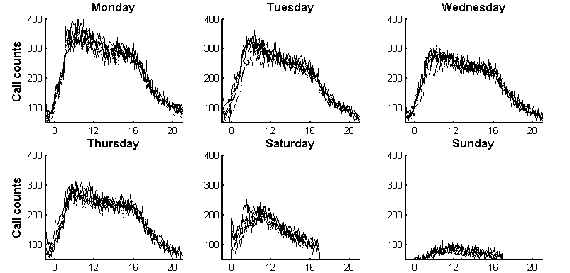
Figure 1: Arrival count in five-minutes resolution for six successive weeks, grouped according to weekday (Friday was omitted due to space constraints). There is a clear difference between workdays, Saturdays, and Sundays. For the working days, it seems that there is some common pattern. Between 7 AM and 10 AM the call count rises sharply to its peak. Then it decreases gradually until 4 PM. From 4 PM to 5 PM there is a rapid decrease followed by a more gradual decrease from 5 PM until 12 AM. The call counts are smaller for Saturday and much smaller for Sunday. Note also that the main activity hours for weekends are 8 AM to 5 PM, as expected.

The third example explores the arrival process during weekends between March and October 2003. There are 67 days in the data set (excluding one day with incomplete data). As can be seen from Figure 1, the weekend behavior is different from that of the working days, and there is a Saturday pattern and a Sunday pattern. The data for this example consists of the arrival counts at fifteen-minutes resolution between 8 AM and 5 PM. The change in interval length from the previous two examples is due to the decreased call-counts. The change in day length is due to the low activity in early morning and late afternoon hours on weekends (see Figure 1).

In the first and second examples, we used the first 100 weekdays as the training set and the last 64 weekdays as the test set. For each day from day 101 to day 164, we extracted the same-weekday information from the preceding 100 days. Thus, for each day of the week we have about 20 training days. For the third example, the test set consists of weekend days 41 to 67 while the training set for each day consist of its previous 40 weekend days. Thus, similarly, for each day we have about 20 training days. Additionally, we used the data from day start, up to 10 AM and up to 12 PM. All forecasts were evaluated using the data after 12 PM, which enabled fair comparison between the results of the different cut points (10 AM and 12 PM). We also compare our results to the mean of the preceding days, from 12 PM on.

For a detailed description of the first example’s data, the reader is referred to Weinberg, Brown and Stroud (2007), Section 2. For an explanation of how the second example’s workload process was computed, the reader is referred to Reich (2010). The data for the third example was extracted using SEEStat, which is a software written at the Technion SEELab. We refer the reader to Donin et al. (2006) for a detailed description of the U.S. commercial bank call-center data from which the data for all three examples was extracted. The U.S. bank call-center data is publicly downloaded from SEESLab server.

5.3 Forecast implementation

The forecast was performed by Matlab implementation of the BLUP algorithm from Section 3, where we enable regularization as in (9). For the implementation we used the functional data analysis Matlab library, written by Ramsay and Silverman. The Matlab code, as well as the data sets, are downloadable (see Acknowledgements). The parameters for the forecast were chosen using $10$-fold cross-validation (see end of Section 2). We computed local confidence bands with $95\%$ confidence level using cross-validation, as described in (16). We quantified the results using both Root Mean Squared Error (RMSE) and Average Percent Error (APE), which are defined as follows. For each day $j$, let

$$RMSE_{j}=\left(\frac{1}{K}\sum_{k=1}^{K}(N_{jk}-\hat{N}_{jk})^{2}\right)^{1/2}\quad;\quad APE_{j}=\frac{100}{K}\sum_{k=1}^{K}\frac{|N_{jk}-\hat{N}_{jk}|}{N_{jk}}\,,$$

where $N_{jk}$ is the actual number of calls (mean workload) at the $k$-th time interval of day $j$ in the arrival (workload) process application, $\hat{N}_{jk}$ is the forecast of $N_{jk}$, and $K$ is the number of intervals.

5.4 First example: Arrival process for weekdays data

Forecasting the arrival process for the first example data was studied by both Weinberg, Brown and Stroud (2007) and Shen and Huang (2008). Weinberg, Brown and Stroud assumed that the day patterns behave according to an autoregressive model. The algorithm they suggest first gives a forecast for the current day based on previous days’ data. The algorithm estimates the parameters in the autoregressive model using Bayesian techniques. An update for the continuation of the current day forecast is obtained by conditioning on the data of the current day up to the cut point. We refer to this algorithm as Bayesian update (BU) for short. Similarly, the algorithm by Shen and Huang assumes an autoregressive model and gives a forecast for the current day. They then update this forecast using least-square penalization, assuming an underlying discrete process. We will refer to this algorithm as penalized least square (PLS).

Comparison between the results of all three algorithms for the first data set appears in Table 1. Note that for all of the algorithms and all of the categories there is improvement in the 10 AM and 12 PM forecasts over the forecast based solely on past days. The RMSE mean decreases by about 5-13% for the 10 AM forecast, and by 12-15% for the 12 PM forecast, depending on the algorithm. It should be noted that the algorithms by Weinberg, Brown and Stroud and by Shen and Huang use information from all $100$ previous days and the knowledge of the previous day call counts. In comparison, the BLUP algorithm uses only the same weekday information ($\sim$20 days) and the previous day information is not part of its training set. Nevertheless, the results are similar.

Example 1	Previous day		10 AM				12 PM
RMSE	mean		BU	PLS	BLUP		BU	PLS	BLUP
Minimum	12.46		11.08		11.51		11.07		11.51
Q1	14.11		14.00	13.31	13.51		13.56	13.33	13.27
Median	16.40		15.50	14.87	14.69		14.80	14.60	14.17
Mean	19.11		17.86	16.48	16.83		16.59	16.13	16.15
Q3	21.27		19.87	17.26	17.04		16.58	16.39	15.92
Maximum	68.93		57.72		52.09		53.66		51.03

Table 1: Summary of statistics (minimum, lower quartile (Q1), median, mean, upper quartile (Q3), maximum) of RMSE for the forecast based on the mean of the previous days, and BU, PLS, and BLUP using data up to 10 AM and up to 12 PM for the call arrival data set. The results for BU and PLS were taken from the original papers. No maximum and minimum results were given for PLS.

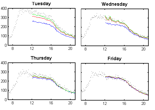
Figure 2: Forecasting results for the week following Labor Day (Sept. 2-5, 2003) for the call arrival process of the first example. Labor Day itself (Monday) does not appear since holiday data is not included in the data set. The black dots represent the true call counts in five-minutes resolution. The forecasts based on previous days, 10 AM data, and 12 PM data are represented by the blue, red, and green lines, respectively.

The forecasting results for the week that follows Labor Day appear in Figure 2. It can be seen that for the Tuesday that follows Labor Day (Monday) the call counts are much higher than usual. This is captured, to some degree, by the 10 AM forecast and much better by the 12 PM forecast. The same phenomenon occurs, with less strength, during the Wednesday and Thursday following Labor Day, until on Friday all the forecasts become roughly the same. It seems that the power of the continuation-of-curve forecasting is exactly in such situations, in which the call counts are substantially different than usual throughout the day, due to either predictable events, such as holidays, or unpredictable events.

5.5 Second example: Workload process for weekdays data

The second example consists of the workload process for weekdays data for the same period as the first example. We forecast the workload process based on these sets of data: previous days’ data, up to 10 AM data, and up to 12 PM data. We refer to this forecast as direct workload forecast since we use past workload estimation as the basis for the forecast. An alternative (and simpler) workload forecasting method was proposed by Aldor-Noiman, Feigin and Mandelbaum (2009). Aldor-Noiman, Feigin and Mandelbaum suggest to forecast the workload by multiplying the forecasted arrival rate by the estimated average service time (see Aldor-Noiman, Feigin and Mandelbaum, 2009, Eq. 21). We refer to this method as indirect workload forecasting.

Comparison between the two methods appears in Table 2. Following Aldor-Noiman, Feigin and Mandelbaum (2009), we estimated the average service time over a 30 minute period for indirect workload computations. Note that the direct workload forecast results are slightly better than the indirect workload forecast in most of the categories. Also note that in almost all categories, there is an improvement in the 10 AM and 12 PM forecasts over the forecast based solely on past days. The RMSE mean decreases by about 11% (9%) for the 10 AM forecast, and by 15% (12%) for the 12 PM forecast for the direct (indirect) forecast. Figure 3 presents a visual comparison between the direct and the indirect forecast methods on a specific day. The two forecasts look roughly the same, which is also true for all other days in this data set.

While in this example there is no significant difference between the direct and indirect workload forecasts, we expect these methods to obtain different forecasts when the arrival rate changes during an average service time. This is true, for example, for arrival and service of patients in emergency rooms. The arrival rates of patients to emergency rooms can change within an hour while the time that a patient spends in emergency room (the “service time”) is typically on the order of hours. As pointed out by Rozenshmidt (2008, Section 6), in such cases, forecasting the workload by the arrival count multiplied by the average service time may not be accurate. This is because the number of customers in the system is cumulative, while the arrival count counts only those who arrive in the current time interval. Thus, if the arrival count is lower than it was in the previous time interval and the average service time is long, the workload is underestimated. Similarly, if the arrival count is larger than previously, the workload is overestimated.

Example 2	Day ahead			10 AM			12 PM
RMSE	Workload	Workload		Workload	Workload		Workload	Workload
	(indirect)	(direct)		(indirect)	(direct)		(indirect)	(direct)
Minimum	8.72	8.41		7.98	7.71		7.96	8.50
Q1	10.76	10.58		10.21	10.27		10.21	10.11
Median	12.10	12.26		11.63	11.21		11.66	11.05
Mean	15.97	15.95		14.59	14.26		14.13	13.48
Q3	15.08	15.21		14.53	14.20		13.89	12.76
Maximum	96.09	94.79		95.74	85.11		93.39	71.20

Table 2: Summary of statistics (minimum, lower quartile (Q1), median, mean, upper quartile (Q3), maximum) of RMSE for the forecast based on the mean of the previous days’ data, up to 10 AM data and up to 12 PM data, for the workload data set, for both the indirect and the direct forecast methods using the BLUP.

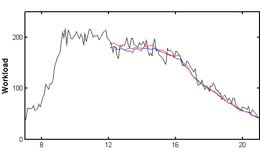
Figure 3: Workload forecasting for Friday, September 5, 2003, using both the direct and the indirect methods. The black curve represents the workload process estimated after observing the data gathered throughout the day. The blue and red curves represents the workload forecasts for the indirect and direct forecasts, respectively, given data up to 12 PM.

5.6 Third example: Arrival process for weekends data

The third example it that of the weekends’ arrivals. The main difference between the first two examples and this one is that the data in this example cannot be considered as data from successive days, due the six day difference between any Sunday and it successive Saturday. Recall that the models considered by Weinberg, Brown and Stroud (2007) and Shen and Huang (2008) have an autoregressive structure. Since this autoregressive structure seems not to hold for this data, the techniques by Weinberg, Brown and Stroud and Shen and Huang are not directly applicable. But even when the autoregressive structure does not hold, the results appearing in Table 3 reveal that forecasting for this data set is still beneficial. Indeed, the RMSE (APE) mean decreases by about 5% (2%) for the 10 AM forecast, and by 10% (4%) for the 12 PM forecast. While these results are not as good as the results in the previous examples, note that the curves in this example begin an hour later and while the call counts are lower during weekends, the arrival rate variance does not change drastically (see Figure 1).

Example 3	RMSE				APE
	Day ahead	10 AM	12 PM		Day ahead	10 AM	12 PM
Minimum	3.66	3.62	3.92		4.47	4.33	4.60
Q1	5.37	5.63	5.05		5.57	5.41	5.64
Median	6.80	7.01	6.87		6.71	6.84	6.31
Mean	7.64	7.19	6.97		7.23	7.10	6.97
Q3	9.01	8.97	8.59		8.83	8.16	7.44
Maximum	16.12	11.84	11.13		12.17	11.80	12.46

Table 3: Summary of statistics (minimum, lower quartile (Q1), median, mean, upper quartile (Q3), maximum) of RMSE and APE for the forecast based on the mean of the previous days and the BLUP, using 10 AM and 12 PM cuts for the weekends data set.

5.7 Confidence bands

Following Weinberg, Brown and Stroud (2007), we introduce the 95% confidence band coverage (COVER) and the average 95% confidence band width (WIDTH). Specifically, for each day $j$, let

$$COVER_{j}=\frac{1}{K}\sum_{k=1}^{K}I\left(F_{L,jk}<N_{jk}<F_{U,jk}\right)\;;\;WIDTH_{j}=\frac{1}{K}\sum_{k=1}^{K}\left(F_{U,jk}-F_{L,jk}\right)\,,$$

where $(F_{L,jk},F_{U,jk})$ is the confidence band of day $j$, evaluated at the beginning of the $k$-th interval (see (16)). The mean coverage and mean width, for all three examples, are presented in Table 4. First, note that for all three examples, the width of the confidence band narrows down as more information is revealed. In other words, the width of the confidence band for the 12 PM forecast is narrower than the width for the 10 AM forecast which, in turn, is narrower than the width for the pervious days’ mean. We also see that the mean coverage becomes more accurate as more information is revealed. Figure 4 depicts the confidence bands for the arrival process on a particular Sunday. Note that the confidence bands for the previous days’ forecast and the 10 AM forecast almost coincide. However, at 12 PM, when enough information on this particular day becomes available, the confidence band narrows down and does capture the underlying behavior.

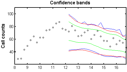
Figure 4: Confidence bands for Sunday, August 10, 2003. The black dots represent the true call counts in fifteen-minutes resolution. The confidence bands based on previous days, 10 AM data, and 12 PM data are represented by the blue, red, and green lines, respectively.

	Coverage				Width
	Example 1	Example 2	Example 3		Example 1	Example 2	Example 3
Mean	93.19%	91.69%	98.15%		79.73	62.80	40.15
10 AM	94.14%	92.27%	98.64%		74.99	56.45	39.53
12 PM	94.86%	93.08%	96.49%		73.07	55.95	31.40

Table 4: The mean confidence band coverage and the mean width for the forecasts based on the previous days’ mean, the 10 AM cut and the 12 PM cut for the arrival process on the working days data set (Example 1), the workload process on the working days data set (Example 2) and the arrival process on the weekends data set (Example 3).

Summarizing, using call center data, we demonstrated that forecasting of curve continuation can be achieved successfully by the proposed BLUP. We also showed that confidence bands for such forecasts can be obtained using cross-validation.

6 Concluding Remarks

We have constructed the best linear unbiased predictor (BLUP) for the continuation of a curve. We now add the following comments regarding the construction of the BLUP and its application to call center data.

First, in our analysis we have used a spline model to describe the functions. This is not required for the construction of the BLUP, and the proof of Theorem 3.4 holds for any function space of finite dimension. However, as discussed previously, there are two main advantages of using spline representation. First, the computation of the covariance operators, for $S_{1},S_{2}$ and $S$ and between them, as well as the pseudo-inverse covariance operator $\Gamma_{11}^{+}$, are all computationally simple when working with splines. Second, the representation of the restriction of a function to a partial segment does not suffer from collinearity of the basis functions, which can be the case for a more general setting. Indeed, the number of basis elements can be reduced significantly in the spline function model, depending on the number of knots in the partial segment, while the number of basis elements could remain the same in a more general model.

Second, we have assumed that the random function $X$ lies within a function space of (possibly large) finite-dimension. While this is a restrictive assumption, there are some difficulties with the BLUP definition (and computation) for a random function that lies in an infinite-dimensional space. The main difficulty is that inverting the covariance operator (as done in Lemma 3.3 for finite dimension) is problematic since the inverse of the covariance operator need not be bounded and may not exists. However, we believe that characterization of the BLUP in the infinite-dimension case is possible under some conditions. Further research is required to address this question.

Finally, in this work we forecasted the continuation of the workload process. As discussed in Feldman et al. (2008) and Reich (2010), the workload process is a more appropriate candidate than the arrival process, as a basis for determining staffing levels in call centers. This work, along with Aldor-Noiman, Feigin and Mandelbaum (2009) and Reich (2010), are the first steps in exploring direct forecasting of the workload process, but more remains to done (see, for example Whitt, 1999; Zeltyn et al., 2009).

Appendix A Proofs

A.1 Lemma A.1

Lemma A.1.

Let $T$ be a $n\times p$ matrix of rank $s$ and let $L$ be a $p\times p$ positive definite diagonal matrix. Then the following assertions are true

1. $T^{\prime}T(T^{\prime}T)^{+}T^{\prime}=T^{\prime}$

2. $T^{\prime}LT(T^{\prime}LT)^{+}T^{\prime}=T^{\prime}$

3. $(T^{\prime}T)^{+}=T^{\prime}\left((TT^{\prime})^{+}\right)^{2}T$

Proof.

1. If $T^{\prime}T$ is invertible then $(T^{\prime}T)^{+}=(T^{\prime}T)^{-1}$ and the result follows. Otherwise, let $U\Lambda V^{\prime}$ be the svd (singular value decomposition, see Golub and Loan, 1983) of $T$ where $U$ and $V$ are orthonormal columns matrices of size $n\times s$ and $p\times s$ respectively, and $\Lambda$ is a $s\times s$ positive definite diagonal matrix. Then

   $$T^{\prime}T(T^{\prime}T)^{+}T^{\prime} = (V\Lambda U^{\prime})(U\Lambda V^{\prime})\big{(}(V\Lambda U^{\prime})(U\Lambda V^{\prime})\big{)}^{+}V\Lambda U^{\prime}$$

   $$= V\Lambda^{2}V^{\prime}(V\Lambda^{2}V^{\prime})^{+}V\Lambda U^{\prime}\,.$$

   Since $\Lambda$ is invertible and $V$ has orthonormal columns $(V\Lambda^{2}V^{\prime})^{+}=V\Lambda^{-2}V^{\prime}$. Hence

   $$T^{\prime}T(T^{\prime}T)^{+}T^{\prime}=V\Lambda^{2}V^{\prime}V\Lambda^{-2}V^{\prime}V\Lambda U^{\prime}=V\Lambda U^{\prime}=T^{\prime}\,.$$

2. Denote $W=L^{1/2}T$, then $T^{\prime}LT(T^{\prime}LT)^{+}T^{\prime}=W^{\prime}W(W^{\prime}W)^{+}W^{\prime}L^{-1/2}$. Using 1., we obtain $W^{\prime}W(W^{\prime}W)^{+}W^{\prime}L^{-1/2}=W^{\prime}L^{-1/2}=T^{\prime}$.

3. Since $TT^{\prime}$ is a positive semi-definite matrix, $TT^{\prime}$ has a spectral representation of the form $TT^{\prime}=\sum_{i=1}^{s}\lambda_{i}v_{i}v_{i}^{\prime}$ where $s\leq\min\{n,p\}$, $\lambda_{i}>0$ and $\{v_{i}\}$ is an orthonormal set of vectors. Note that $TT^{\prime}v_{i}=\lambda_{i}v_{i}$ and hence $T^{\prime}T(T^{\prime}v_{i})=\lambda_{i}T^{\prime}v_{i}$. Moreover $\left\|T^{\prime}v_{i}\right\|^{2}=v_{i}^{\prime}TT^{\prime}v_{i}=v_{i}^{\prime}(\lambda_{i}v_{i})=\lambda_{i}$. Hence, we obtained that $\left\{T^{\prime}v_{i}/\sqrt{\lambda_{i}}\right\}$ is the set of orthonormal eigenvectors of $T^{\prime}T$ with the respective non-zero eigenvalues $\{\lambda_{i}\}$. Thus,

   $$T^{\prime}T=\sum_{i=1}^{s}\lambda_{i}\frac{T^{\prime}v_{i}}{\sqrt{\lambda_{i}}}\left(\frac{T^{\prime}v_{i}}{\sqrt{\lambda_{i}}}\right)^{\prime}=T^{\prime}\left(\sum_{i=1}^{s}v_{i}v_{i}^{\prime}\right)T\,.$$

   Using the spectral representation we also have

   $$T^{\prime}\left((TT^{\prime})^{+}\right)^{2}T=T^{\prime}\left(\sum_{i=1}^{s}\lambda_{i}^{-2}v_{i}v_{i}^{\prime}\right)T\,.$$

   In order to show that $(T^{\prime}T)^{+}=T^{\prime}\left((TT^{\prime})^{+}\right)^{2}T$ we need to show the following (see Golub and Loan, 1983):

   1. $(T^{\prime}T)\left(T^{\prime}\left((TT^{\prime})^{+}\right)^{2}T\right)(T^{\prime}T)=(T^{\prime}T)$

   2. $\left(T^{\prime}\left((TT^{\prime})^{+}\right)^{2}T\right)(T^{\prime}T)(T^{\prime}\left((TT^{\prime})^{+}\right)^{2}T)=\left(T^{\prime}\left((TT^{\prime})^{+}\right)^{2}T\right)$

   3. $\left((T^{\prime}T)\left(T^{\prime}\left((TT^{\prime})^{+}\right)^{2}T\right)\right)^{\prime}=(T^{\prime}T)(T^{\prime}\left((TT^{\prime})^{+}\right)^{2}T)$

   4. $\left(\left(T^{\prime}\left((TT^{\prime})^{+}\right)^{2}T\right)(T^{\prime}T)\right)^{\prime}=(T^{\prime}\left((TT^{\prime})^{+}\right)^{2}T)(T^{\prime}T)$

   In order to see (a), note that

   $$(T^{\prime}T)\left(T^{\prime}\left((TT^{\prime})^{+}\right)^{2}T\right)(T^{\prime}T) = T^{\prime}(TT^{\prime})\left(\sum_{i=1}^{s}\lambda_{i}^{-2}v_{i}v_{i}^{\prime}\right)(TT^{\prime})T$$

   $$= T^{\prime}\left(\sum_{i=1}^{s}\lambda_{i}v_{i}v_{i}^{\prime}\right)\left(\sum_{i=1}^{s}\lambda_{i}^{-2}v_{i}v_{i}^{\prime}\right)\left(\sum_{i=1}^{s}\lambda_{i}v_{i}v_{i}^{\prime}\right)T$$

   $$= T^{\prime}\left(\sum_{i=1}^{s}\ v_{i}v_{i}^{\prime}\right)T=T^{\prime}T\,.$$

   Similarly, for (b), we have

   $$\left(T^{\prime}\left((TT^{\prime})^{+}\right)^{2}T\right) (T^{\prime}T)\left(T^{\prime}\left((TT^{\prime})^{+}\right)^{2}T\right)=$$

   $$=T^{\prime}\left(\sum_{i=1}^{s}\lambda_{i}^{-2}v_{i}v_{i}^{\prime}\right)(TT^{\prime})^{2}\left(\sum_{i=1}^{s}\lambda_{i}^{-2}v_{i}v_{i}^{\prime}\right)T$$

   $$=T^{\prime}\left(\sum_{i=1}^{s}\lambda_{i}^{-2}v_{i}v_{i}^{\prime}\right)\left(\sum_{i=1}^{s}\lambda_{i}v_{i}v_{i}^{\prime}\right)^{2}\left(\sum_{i=1}^{s}\lambda_{i}^{-2}v_{i}v_{i}^{\prime}\right)T$$

   $$=T^{\prime}\left(\sum_{i=1}^{s}\lambda_{i}^{-2}v_{i}v_{i}^{\prime}\right)T=T^{\prime}\left((TT^{\prime})^{+}\right)^{2}T\,.$$

   For (c),

   $$\left((T^{\prime}T)\left(T^{\prime}\left((TT^{\prime})^{+}\right)^{2}T\right)\right)^{\prime} = \left(T^{\prime}(TT^{\prime})\left(\sum_{i=1}^{s}\lambda_{i}^{-2}v_{i}v_{i}^{\prime}\right)T\right)^{\prime}=\left(T^{\prime}\left(\sum_{i=1}^{s}\lambda_{i}^{-1}v_{i}v_{i}^{\prime}\right)T\right)^{\prime}$$

   $$= T^{\prime}\left(\sum_{i=1}^{s}\lambda_{i}^{-1}v_{i}v_{i}^{\prime}\right)T=(T^{\prime}T)\left(T^{\prime}\left((TT^{\prime})^{+}\right)^{2}T\right)\,.$$

   Finally, (d) is shown similarly to (c).

∎

A.2 Proof of Lemma 3.3

Proof.

By (2) we may write $Y_{1}(t)-\mu(t)=\bm{b}_{\bm{1}}(t)^{\prime}(A_{1}\bm{h}+B_{1}\bm{\epsilon})$. Hence,

$$\left(\Gamma_{11}\Gamma_{11}^{+}\right. \left.(A_{1}\bm{h}+B_{1}\bm{\epsilon})\right)(t)=$$

$$=\bm{b}_{\bm{1}}(t)^{\prime}G_{11}W_{1}W_{1}^{-1}G_{11}^{+}(A_{1}\bm{h}+B_{1}\bm{\epsilon})$$

$$=\bm{b}_{\bm{1}}(t)^{\prime}G_{11}G_{11}^{+}(A_{1}\bm{h}+B_{1}\bm{\epsilon})$$

$$=\bm{b}_{\bm{1}}(t)^{\prime}[A_{1},B_{1}]\left[\begin{array}[]{cc}L&0\\ 0&\Sigma\end{array}\right]\left[\begin{array}[]{c}A_{1}^{\prime}\\ B_{1}^{\prime}\\ \end{array}\right]\left([A_{1},B_{1}]\left[\begin{array}[]{cc}L&0\\ 0&\Sigma\end{array}\right]\left[\begin{array}[]{c}A_{1}^{\prime}\\ B_{1}^{\prime}\\ \end{array}\right]\right)^{+}\left[\begin{array}[]{c}A_{1}\bm{h}\\ B_{1}\bm{\epsilon}\\ \end{array}\right]$$

and the result follows from Lemma A.1.

Substituting $\bm{h}=LA_{2}^{\prime}$ and $\bm{\epsilon}=0$ in the last equation, we also obtain

$$G_{11}G_{11}^{+}g_{12}=\Gamma_{11}G_{11}^{+}(A_{1}LA_{2}^{\prime}+B_{1}\textbf{0})=g_{12}\,.$$ (17)

∎

References

- Aldor-Noiman, Feigin and Mandelbaum (2009) {bunpublished}[author] \bauthor\bsnmAldor-Noiman, \bfnmS.\binitsS., \bauthor\bsnmFeigin, \bfnmP. D.\binitsP. D. and \bauthor\bsnmMandelbaum, \bfnmA.\binitsA. (\byear2009). \btitleWorkload forecasting for a call center: Methodology and a case study. \bnoteTo appear. \endbibitem
- Antoniadis, Paparoditis and Sapatinas (2006) {barticle}[author] \bauthor\bsnmAntoniadis, \bfnmA.\binitsA., \bauthor\bsnmPaparoditis, \bfnmE.\binitsE. and \bauthor\bsnmSapatinas, \bfnmT.\binitsT. (\byear2006). \btitleA functional waveletkernel approach for time series prediction. \bjournalJournal of the Royal Statistical Society: Series B (Statistical Methodology) \bvolume68 \bpages837–857. \endbibitem
- Besse, Cardot and Ferraty (1997) {barticle}[author] \bauthor\bsnmBesse, \bfnmP.\binitsP., \bauthor\bsnmCardot, \bfnmH.\binitsH. and \bauthor\bsnmFerraty, \bfnmF.\binitsF. (\byear1997). \btitleSimultaneous non-parametric regressions of unbalanced longitudinal data. \bjournalComputational Statistics & Data Analysis \bvolume24 \bpages255–270. \endbibitem
- Besse, Cardot and Stephenson (2000) {barticle}[author] \bauthor\bsnmBesse, \bfnmPhilippe C.\binitsP. C., \bauthor\bsnmCardot, \bfnmHerve\binitsH. and \bauthor\bsnmStephenson, \bfnmDavid B.\binitsD. B. (\byear2000). \btitleAutoregressive forecasting of some functional climatic variations. \bjournalScandinavian Journal of Statistics \bvolume27 \bpages673–687. \endbibitem
- de Boor (2001) {bbook}[author] \bauthor\bparticlede \bsnmBoor, \bfnmC.\binitsC. (\byear2001). \btitleA practical guide to splines, \beditionRevised ed. \bseriesApplied Mathematical Sciences. \bpublisherSpringer-Verlag New York. \endbibitem
- Donin et al. (2006) {bmisc}[author] \bauthor\bsnmDonin, \bfnmO.\binitsO., \bauthor\bsnmFeigin, \bfnmP. D.\binitsP. D., \bauthor\bsnmMandelbaum, \bfnmA.\binitsA., \bauthor\bsnmZeltyn, \bfnmS.\binitsS., \bauthor\bsnmTrofimov, \bfnmV.\binitsV., \bauthor\bsnmIshay, \bfnmE.\binitsE., \bauthor\bsnmKhudiakov, \bfnmP.\binitsP. and \bauthor\bsnmNadjharov, \bfnmE.\binitsE. (\byear2006). \btitleThe Call Center of US Bank . \bnoteAvaliable at http://ie.technion.ac.il/Labs/Serveng/files/The_Call_Center_of_US_Bank.pdf. \endbibitem
- Feldman et al. (2008) {barticle}[author] \bauthor\bsnmFeldman, \bfnmZ.\binitsZ., \bauthor\bsnmMandelbaum, \bfnmA.\binitsA., \bauthor\bsnmMassey, \bfnmW. A.\binitsW. A. and \bauthor\bsnmWhitt, \bfnmW.\binitsW. (\byear2008). \btitleStaffing of Time-Varying Queues to Achieve Time-Stable Performance. \bjournalManagement Science \bvolume54 \bpages324–338. \endbibitem
- Gans, Koole and Mandelbaum (2003) {barticle}[author] \bauthor\bsnmGans, \bfnmN.\binitsN., \bauthor\bsnmKoole, \bfnmG.\binitsG. and \bauthor\bsnmMandelbaum, \bfnmA.\binitsA. (\byear2003). \btitleTelephone Call Centers: Tutorial, Review, and Research Prospects. \bjournalManufacturing Service Operations Management \bvolume5 \bpages79-141. \endbibitem
- Golub and Loan (1983) {bbook}[author] \bauthor\bsnmGolub, \bfnmG. H.\binitsG. H. and \bauthor\bsnmLoan, \bfnmC. F. Van\binitsC. F. V. (\byear1983). \btitleMatrix computations. \bpublisherJohns Hopkins University Press, \baddressBaltimore, Maryland. \endbibitem
- Hoerl and Kennard (1970) {barticle}[author] \bauthor\bsnmHoerl, \bfnmA. E.\binitsA. E. and \bauthor\bsnmKennard, \bfnmR. W.\binitsR. W. (\byear1970). \btitleRidge regression: biased estimation for nonorthogonal problems. \bjournalTechnometrics \bvolume12 \bpages55–67. \endbibitem
- Knafl, Sacks and Ylvisaker (1985) {barticle}[author] \bauthor\bsnmKnafl, \bfnmG.\binitsG., \bauthor\bsnmSacks, \bfnmJ.\binitsJ. and \bauthor\bsnmYlvisaker, \bfnmD.\binitsD. (\byear1985). \btitleConfidence bands for regression functions. \bjournalJournal of the American Statistical Association \bvolume80 \bpages683–691. \endbibitem
- Kneip (1994) {barticle}[author] \bauthor\bsnmKneip, \bfnmA.\binitsA. (\byear1994). \btitleNonparametric estimation of common regressors for similar curve data. \bjournalThe Annals of Statistics \bvolume22 \bpages1386–1427. \endbibitem
- Marsaglia (1964) {barticle}[author] \bauthor\bsnmMarsaglia, \bfnmG.\binitsG. (\byear1964). \btitleConditional means and covariances of normal variables with singular covariance matrix. \bjournalJournal of the American Statistical Association \bvolume59 \bpages1203–1204. \endbibitem
- Ramsay and Silverman (2002) {bbook}[author] \bauthor\bsnmRamsay, \bfnmJ.\binitsJ. and \bauthor\bsnmSilverman, \bfnmB. W.\binitsB. W. (\byear2002). \btitleApplied functional data analysis: methods and case studies, \bedition2nd ed. \bseriesSpringer Series in Statistics. \bpublisherSpringer-Verlag New York. \endbibitem
- Ramsay and Silverman (2005) {bbook}[author] \bauthor\bsnmRamsay, \bfnmJ.\binitsJ. and \bauthor\bsnmSilverman, \bfnmB. W.\binitsB. W. (\byear2005). \btitleFunctional data analysis. \bseriesSpringer Series in Statistics. \bpublisherSpringer-Verlag New York. \endbibitem
- Reich (2010) {bmastersthesis}[author] \bauthor\bsnmReich, \bfnmM.\binitsM. (\byear2010). \btitleThe workload process: modelling, inference and applications \btypeMaster’s thesis, \bschoolTechnion - Israel Institute of Technology. \bnoteIn preparation. The proposal is avaliable at http://ie.technion.ac.il/serveng/References/references.html. \endbibitem
- Robinson (1991) {barticle}[author] \bauthor\bsnmRobinson, \bfnmG. K.\binitsG. K. (\byear1991). \btitleThat BLUP is a good thing: the estimation of random effects. \bjournalStatistical Science \bvolume6 \bpages15–32. \endbibitem
- Rozenshmidt (2008) {bmastersthesis}[author] \bauthor\bsnmRozenshmidt, \bfnmL.\binitsL. (\byear2008). \btitleOn priority queues with impatient customers: Stationary and time-varying analysis \btypeMaster’s thesis, \bschoolTechnion - Israel Institute of Technology. \bnoteAvaliable at http://iew3.technion.ac.il/serveng/References/thesis_Luba_Eng.pdf. \endbibitem
- Sansone (1991) {bbook}[author] \bauthor\bsnmSansone, \bfnmG.\binitsG. (\byear1991). \btitleOrthogonal functions, \beditionRev. ed. ed. \bpublisherDover Publications,, \baddressNew York. \endbibitem
- Shen (2009) {barticle}[author] \bauthor\bsnmShen, \bfnmH.\binitsH. (\byear2009). \btitleOn modeling and forecasting time series of smooth curves. \bjournalTechnometrics \bvolume51 \bpages227–238. \endbibitem
- Shen and Huang (2008) {barticle}[author] \bauthor\bsnmShen, \bfnmH.\binitsH. and \bauthor\bsnmHuang, \bfnmJ. Z.\binitsJ. Z. (\byear2008). \btitleInterday Forecasting and Intraday Updating of Call Center Arrivals. \bjournalManufacturing Service Operations Management \bvolume10 \bpages391–410. \endbibitem
- Weinberg, Brown and Stroud (2007) {barticle}[author] \bauthor\bsnmWeinberg, \bfnmJ.\binitsJ., \bauthor\bsnmBrown, \bfnmL. D.\binitsL. D. and \bauthor\bsnmStroud, \bfnmJ. R.\binitsJ. R. (\byear2007). \btitleBayesian forecasting of an inhomogeneous poissonprocess with applications to call center data. \bjournalJournal of the American Statistical Association \bvolumeVol. 102. \endbibitem
- Whitt (1999) {barticle}[author] \bauthor\bsnmWhitt, \bfnmW.\binitsW. (\byear1999). \btitleDynamic staffing in a telephone call center aiming to immediately answer all calls. \bjournalOperations Research Letters \bvolume24 \bpages205 - 212. \endbibitem
- Zeltyn (2005) {bphdthesis}[author] \bauthor\bsnmZeltyn, \bfnmS.\binitsS. (\byear2005). \btitleCall centers with impatient customers: Exact analysis and many-server asymptotics of the M/M/n+G queue. \btypePhD thesis, \bschoolTechnion Israel Institute of Technology. \bnoteAvailable at http://ie.technion.ac.il/serveng/References/references.html. \endbibitem
- Zeltyn et al. (2009) {bunpublished}[author] \bauthor\bsnmZeltyn, \bfnmS.\binitsS., \bauthor\bsnmCarmeli, \bfnmB.\binitsB., \bauthor\bsnmGreenshpan, \bfnmO.\binitsO., \bauthor\bsnmMesika, \bfnmY.\binitsY., \bauthor\bsnmWasserkrug, \bfnmS.\binitsS., \bauthor\bsnmVortman, \bfnmP.\binitsP., \bauthor\bsnmMarmor, \bfnmY. N.\binitsY. N., \bauthor\bsnmMandelbaum, \bfnmA.\binitsA., \bauthor\bsnmShtub, \bfnmA.\binitsA., \bauthor\bsnmLauterman, \bfnmT.\binitsT., \bauthor\bsnmSchwartz, \bfnmD.\binitsD., \bauthor\bsnmMoskovitch, \bfnmK.\binitsK., \bauthor\bsnmTzafrir, \bfnmS.\binitsS. and \bauthor\bsnmBasis, \bfnmF.\binitsF. (\byear2009). \btitleSimulation-Based Models of Emergency Departments: Operational, Tactical and Strategic Staffing. \bnoteUnder review. \endbibitem