On the estimation of integrated covariance matrices of high dimensional diffusion processes

Abstract

We consider the estimation of integrated covariance (ICV) matrices of high dimensional diffusion processes based on high frequency observations. We start by studying the most commonly used estimator, the realized covariance (RCV) matrix. We show that in the high dimensional case when the dimension $p$ and the observation frequency $n$ grow in the same rate, the limiting spectral distribution (LSD) of RCV depends on the covolatility process not only through the targeting ICV, but also on how the covolatility process varies in time. We establish a Marčenko–Pastur type theorem for weighted sample covariance matrices, based on which we obtain a Marčenko–Pastur type theorem for RCV for a class $\mathcal{C}$ of diffusion processes. The results explicitly demonstrate how the time variability of the covolatility process affects the LSD of RCV. We further propose an alternative estimator, the time-variation adjusted realized covariance (TVARCV) matrix. We show that for processes in class $\mathcal{C}$, the TVARCV possesses the desirable property that its LSD depends solely on that of the targeting ICV through the Marčenko–Pastur equation, and hence, in particular, the TVARCV can be used to recover the empirical spectral distribution of the ICV by using existing algorithms.

T1Supported in part by DAG (HKUST) and GRF 606811 of the HKSAR.

and

1 Introduction

1.1 Background

Diffusion processes are widely used to model financial asset price processes. For example, suppose that we have multiple stocks, say, $p$ stocks whose price processes are denoted by $S^{(j)}_{t}$ for $j=1,\ldots,p$, and $X_{t}^{(j)}:=\log S_{t}^{(j)}$ are the log price processes. Let $\mathbf{X}_{t}=(X_{t}^{(1)},\ldots,X_{t}^{(p)})^{T}$. Then a widely used model for $\mathbf{X}_{t}$ is [see, e.g., Definition 1 in Barndorff-Nielsen and Shephard (2004)]

$$d\mathbf{X}_{t}={\bolds\mu}_{t}\,dt+\Theta_{t}\,d\mathbf{W}_{t},$$ (1)

where, $\bolds{\mu}_{t}=(\mu_{t}^{(1)},\ldots,\mu_{t}^{(p)})^{T}$ is a $p$-dimensional drift process; $\Theta_{t}$ is a $p\times p$ matrix for any $t$, and is called the (instantaneous) covolatility process; and $\mathbf{W}_{t}$ is a $p$-dimensional standard Brownian motion.

The integrated covariance (ICV) matrix

$${\Sigma_{p}:=\int_{0}^{1}\Theta_{t}\Theta_{t}^{T}\,dt}$$

is of great interest in financial applications, which in the one dimensional case is known as the integrated volatility. A widely used estimator of the ICV matrix is the so-called realized covariance (RCV) matrix, which is defined as follows. Assume that we can observe the processes $X^{(j)}_{t}$’s at high frequency synchronously, say, at time points $\tau_{n,\ell}$:

$$X^{(j)}_{\tau_{n,\ell}}\bigl{(}\mbox{$=$}\log S^{(j)}_{\tau_{n,\ell}}\bigr{)},\qquad\ell=0,1,\ldots,n,j=1,\ldots,p,$$

then the RCV matrix is defined as

$$\Sigma^{\mathrm{RCV}}_{p}:=\sum_{\ell=1}^{n}\Delta\mathbf{X}_{\ell}(\Delta\mathbf{X}_{\ell})^{T}\qquad$$ (3)

$$\eqntext{\mbox{where }\Delta\mathbf{X}_{\ell}=\pmatrix{\Delta X^{(1)}_{\ell}\cr\vdots\cr\Delta X^{(p)}_{\ell}}:=\pmatrix{X^{(1)}_{\tau_{n,\ell}}-X^{(1)}_{\tau_{n,\ell-1}}\cr\vdots\cr X^{(p)}_{\tau_{n,\ell}}-X^{(p)}_{\tau_{n,\ell-1}}}.}$$

In the one dimensional case, the RCV matrix reduces to the realized volatility. Thanks to its nice convergence to the ICV matrix as the observation frequency $n$ goes to infinity [see Jacod and Protter (1998)], the RCV matrix is highly appreciated in both academic research and practical applications.

Remark 1.

The tick-by-tick data are usually not observed synchronously, and moreover are contaminated by market microstructure noise. On sparsely sampled data (e.g., 5-minute data for some highly liquid assets, or subsample from data synchronized by refresh times [Barndorff-Nielsen et al. (2011)]), the theory in this paper should be readily applicable, just as one can use the realized volatility based on sparsely sampled data to estimate the integrated volatility; see, for example, Andersen et al. (2001).

1.2 Large dimensional random matrix theory (LDRMT)

Having a good estimate of the ICV matrix $\Sigma_{p}$, in particular, its spectrum (i.e., its set of eigenvalues $\{\lambda_{j}\dvtx j=1,\ldots,p\}$), is crucial in many applications such as principal component analysis and portfolio optimization (see, e.g., the pioneer work of Markowitz (1952, 1959) and a more recent work [Bai, Liu and Wong (2009)]). When the dimension $p$ is high, it is more convenient to study, instead of the $p$ eigenvalues $\{\lambda_{j}\dvtx j=1,\ldots,p\}$, the associated empirical spectral distribution (ESD)

$$F^{\Sigma_{p}}(x):=\frac{1}{p}\#\{j\dvtx\lambda_{j}\leq x\},\qquad x\in\mathbb{R}.$$

A naive estimator of the spectrum of the ICV matrix $\Sigma_{p}$ is the spectrum of the RCV matrix $\Sigma^{\mathrm{RCV}}_{p}$. In particular, one wishes that the ESD $F^{\Sigma^{\mathrm{RCV}}_{p}}$ of $\Sigma^{\mathrm{RCV}}_{p}$ would approximate $F^{\Sigma_{p}}$ well when the frequency $n$ is sufficiently high. From the large dimensional random matrix theory (LDRMT), we now understand quite well that in the high dimensional setting this good wish won’t come true. For example, in the simplest case when the drift process is 0, covolatility process is constant, and observation times $\tau_{n,\ell}$ are equally spaced, namely, $\tau_{n,\ell}=\ell/n$, we are in the setting of estimating the usual covariance matrix using the sample covariance matrix, given $n$ i.i.d. $p$-dimensional observations $(\Delta\mathbf{X}_{\ell})_{\ell=1,\ldots,n}$. From LDRMT, we know that if $p/n$ converges to a non-zero number and the ESD $F^{\Sigma_{p}}$ of the true covariance matrix converges, then the ESD $F^{\Sigma^{\mathrm{RCV}}_{p}}$ of the sample covariance matrix also converges; see, for example, Marčenko and Pastur (1967), Yin (1986), Silverstein and Bai (1995) and Silverstein (1995). The relationship between the limiting spectral distribution (LSD) of $\Sigma^{\mathrm{RCV}}_{p}$ in this case and the LSD of $\Sigma_{p}$ can be described by a Marčenko–Pastur equation through Stieltjes transforms, as follows.

Proposition 1 ([Theorem 1.1 of Silverstein (1995)]).

Assume on a common probability space:

for $p=1,2,\ldots$ and for $1\leq\ell\leq n$, $\mathbf{Z}^{(p)}_{\ell}=(Z^{(p,j)}_{\ell})_{1\leq j\leq p}$ with $Z^{(p,j)}_{\ell}$ i.i.d. with mean 0 and variance 1;

$n=n(p)$ with $y_{n}:=p/n\rightarrow y>0$ as $p\rightarrow\infty$;

$\Sigma_{p}$ is a (possibly random) nonnegative definite $p\times p$ matrix such that its ESD $F^{\Sigma_{p}}$ converges almost surely in distribution to a probability distribution $H$ on $[0,\infty)$ as $p\rightarrow\infty$;

$\Sigma_{p}$ and $\mathbf{Z}^{(p)}_{\ell}$’s are independent. Let $\Sigma_{p}^{1/2}$ be the (nonnegative) square root matrix of $\Sigma_{p}$ and $S_{p}:=1/n\times\sum_{\ell=1}^{n}\Sigma_{p}^{1/2}\mathbf{Z}^{(p)}_{\ell}(\mathbf{Z}^{(p)}_{\ell})^{T}\Sigma_{p}^{1/2}$. Then, almost surely, the ESD of $S_{p}$ converges in distribution to a probability distribution $F$, which is determined by $H$ in that its Stieltjes transform

$$m_{F}(z):=\int_{\lambda\in\mathbb{R}}\frac{1}{\lambda-z}\,dF(\lambda),\qquad z\in\mathbb{C}_{+}:=\{z\in\mathbb{C}\dvtx\operatorname{Im}(z)>0\}$$

solves the equation

$$m_{F}(z)=\int_{\tau\in\mathbb{R}}\frac{1}{\tau(1-y(1+zm_{F}(z)))-z}\,dH(\tau).$$ (4)

In the special case when $\Sigma_{p}=\sigma^{2}I_{p\times p}$, where $I_{p\times p}$ is the $p\times p$ identity matrix, the LSD $F$ can be explicitly expressed as follows.

Proposition 2 ([see, e.g., Theorem 2.5 in Bai (1999)]).

Suppose that $\mathbf{Z}^{(p)}_{\ell}$’s are as in the previous proposition, and $\Sigma_{p}=\sigma^{2}I_{p\times p}$ for some $\sigma^{2}>0$. Then the LSD $F$ has density

$$p(x)=\frac{1}{2\pi\sigma^{2}xy}\sqrt{(b-x)(x-a)}\qquad\mbox{if }a\leq x\leq b,$$

and a point mass $1-1/y$ at the origin if $y>1$, where

$$a=a(y)=\sigma^{2}\bigl{(}1-\sqrt{y}\bigr{)}^{2}\quad\mbox{and}\quad b=b(y)=\sigma^{2}\bigl{(}1+\sqrt{y}\bigr{)}^{2}.$$ (5)

The LSD $F$ in this proposition is called the Marčenko–Pastur law with ratio index $y$ and scale index $\sigma^{2}$, and will be denoted by MP${}^{(y,\sigma^{2})}$ in this article.

1.3 Back to the stochastic volatility case

In practice, the covolatility process is typically not constant. For example, it is commonly observed that the stock intraday volatility tends to be U-shaped [see, e.g., Admati and Pfleiderer (1988), Andersen and Bollerslev (1997)] or exhibits some other patterns [see, e.g., Andersen and Bollerslev (1998)]. In this article, we shall allow them to be not only varying in time but also stochastic. Furthermore, we shall allow the observation times $\tau_{n,\ell}$ to be random. These generalizations make our study to be different in nature from the LDRMT: in LDRMT the observations are i.i.d.; in our setting, the observations $(\Delta\mathbf{X}_{\ell})_{\ell=1,\ldots,n}$ may, first, be dependant with each other, and second, have different distributions because (i) the covolatility process may vary over time, and (ii) the observation durations $\Delta\tau_{\ell}:=\tau_{n,\ell}-\tau_{n,\ell-1}$ may be different.

In general, for any time-varying covolatility process $\Theta_{t}$, we associate it with a constant covolatility process given by the square root of the ICV matrix

$$\Theta^{0}_{t}:=\sqrt{\int_{0}^{1}\Theta_{s}\Theta_{s}^{T}ds}\qquad\mbox{for all }t\in[0,1].$$ (6)

Let $\mathbf{X}_{t}^{0}$ be defined by replacing $\Theta_{t}$ with the constant covolatility process $\Theta^{0}_{t}$ (and replacing $\mu_{t}$ with 0, and $\mathbf{W}_{t}$ with another independent Brownian motion, if necessary) in (1). Observe that $\mathbf{X}_{t}$ and $\mathbf{X}_{t}^{0}$ share the same ICV matrix at time 1. Based on $\mathbf{X}_{t}^{0}$, we have an associated RCV matrix

$$\Sigma^{\mathrm{RCV}^{0}}_{p}=\sum_{\ell=1}^{n}\Delta\mathbf{X}^{0}_{\ell}(\Delta\mathbf{X}^{0}_{\ell})^{T},$$ (7)

which is estimating the same ICV matrix as $\Sigma^{\mathrm{RCV}}_{p}$.

Since $\Sigma^{\mathrm{RCV}}_{p}$ and $\Sigma^{\mathrm{RCV}^{0}}_{p}$ are based on the same estimation method and share the same targeting ICV matrix, it is desirable that their ESDs have similar properties. In particular, based on the results in LDRMT and the discussion about constant covolatility case in Section 1.2, we have the following property for $\Sigma^{\mathrm{RCV}^{0}}_{p}$: if the ESD $F^{\Sigma_{p}}$ converges, then so does $F^{\Sigma^{\mathrm{RCV}^{0}}_{p}}$; moreover, their limits are related to each other via the Marčenko–Pastur equation (4). Does this property also hold for $\Sigma^{\mathrm{RCV}}_{p}$? Our first result (Proposition 3) shows that even in the most ideal case when the covolatility process has the form $\Theta_{t}=\gamma_{t}\cdot I_{p\times p}$ for some deterministic (scalar) function $\gamma_{t}$, such convergence results may not hold for $\Sigma^{\mathrm{RCV}}_{p}$. In particular, the limit of $F^{\Sigma^{\mathrm{RCV}}_{p}}$ (when it exists) changes according to how the covolatility process evolves over time.

This leads to the following natural and interesting question: how does the LSD of RCV matrix depend on the time-variability of the covolatility process? Answering this question in a general context without putting any structural assumption on the covolatility process seems to be rather challenging, if not impossible. For a class $\mathcal{C}$ (see Section 2) of processes, we do establish a result for RCV matrices that’s analogous to the Marčenko–Pastur theorem (see Proposition 5), which demonstrates clearly how the time-variability of the covolatility process affects the LSD of RCV matrix. Proposition 5 is proved based on Theorem 1, which is a Marčenko–Pastur type theorem for weighted sample covariance matrices. These results, in principle, allow one to recover the LSD of ICV matrix based on that of RCV matrix.

Estimating high dimensional ICV matrices based on high frequency data has only recently started to gain attention. See, for example, Wang and Zou (2010); Tao et al. (2011) who made use of data over long time horizons by proposing a method incorporating low-frequency dynamics; and Fan, Li and Yu (2011) who studied the estimation of ICV matrices for portfolio allocation under gross exposure constraint. In Wang and Zou (2010), under sparsity assumptions on the ICV matrix, banding/thresholding was innovatively used to construct consistent estimators of the ICV matrix in the spectral norm sense. In particular, when the sparsity assumptions are satisfied, their estimators share the same LSD as the ICV matrix. It remains an open question that when the sparsity assumptions are not satisfied, whether one can still make good inference about the spectrum of ICV matrix. For processes in class $\mathcal{C}$ (see Section 2), whose ICV matrices do not need to be sparse, we propose a new estimator, the time-variation adjusted realized covariance (TVARCV) matrix. We show that the TVARCV matrix has the desirable property that its LSD exists provided that the LSD of ICV matrix exists, and furthermore, the two LSDs are related to each other via the Marčenko–Pastur equation (4) (see Theorem 2). Therefore, the TVARCV matrix can be used, for example, to recover the LSD of ICV matrix by inverting the Marčenko–Pastur equation using existing algorithms.

The rest of the paper is organized as the following: theoretical results are presented in Section 2, proofs are given in Section 3, simulation studies in Section 4, and conclusion and discussions in Section 5.

Notation. For any matrix $A$, $\|A\|=\sqrt{\lambda_{\max}(AA^{*})}$ denotes its spectral norm. For any Hermitian matrix $A$, $F^{A}$ stands for its ESD. For two matrices $A$ and $B$, we write $A\leq B$ ($A\geq B$, resp.) if $B-A$ ($A-B$, resp.) is a nonnegative definite matrix. For any interval $I\subseteq[0,\infty)$, and any metric space $S$, $D(I;S)$ stands for the space of càdlàg functions from $I$ to $S$. Additionally, $i=\sqrt{-1}$ stands for the imaginary unit, and for any $z\in\mathbb{C}$, we write $\operatorname{Re}(z),\operatorname{Im}(z)$ as its real part and imaginary part, respectively, and $\overline{z}$ as its complex conjugate. We also denote $\mathbb{R}_{+}=\{a\in\mathbb{R}\dvtx a>0\}$, $\mathbb{C}_{+}=\{z\in\mathbb{C}\dvtx\allowbreak\operatorname{Re}(z)>0\}$ and $Q_{1}=\{z\in\mathbb{C}\dvtx\operatorname{Re}(z)\geq 0,\operatorname{Im}(z)\geq 0\}$. We follow the custom of writing $f\sim g$ to mean that the ratio $f/g$ converges to 1. Finally, throughout the paper, $c,C,C_{1},C^{\prime}$ etc. denote generic constants whose values may change from line to line.

2 Main results

2.1 Dependance of the LSD of RCV matrix on the time-variability of covolatility process

Proposition 1 asserts that the ESD of sample covariance matrix converges to a limiting distribution which is uniquely determined by the LSD of the underlying covariance matrix. Unfortunately, Proposition 1 does not apply to our case, since the observations $\Delta\mathbf{X}_{\ell}$ under our general diffusion process setting are not i.i.d. Proposition 3 below shows that even in the following most ideal case, the RCV matrix does not have the desired convergence property.

Proposition 3.

Suppose that for all $p$, $\mathbf{X}_{t}=\mathbf{X}^{(p)}_{t}$ is a $p$-dimensional process satisfying

$$d\mathbf{X}_{t}=\gamma_{t}\,d\mathbf{W}_{t},\qquad t\in[0,1],$$ (8)

where $\gamma_{t}>0$ is a nonrandom (scalar) càdlàg process. Let $\sigma^{2}=\int_{0}^{1}\gamma_{t}^{2}\,dt$, and so that the ICV matrix $\Sigma_{p}$ is $\sigma^{2}I_{p\times p}$. Assume further that the observation times $\tau_{n,\ell}$ are equally spaced, that is, $\tau_{n,\ell}=\ell/n$, and that the RCV matrix $\Sigma^{\mathrm{RCV}}_{p}$ is defined by (3). Then so long as $\gamma_{t}$ is not constant on $[0,1)$, for any $\varepsilon>0$, there exists $y_{c}=y_{c}(\gamma,\varepsilon)>0$ such that if $\lim p/n=y\geq y_{c}$,

$$\limsup F^{\Sigma^{\mathrm{RCV}}_{p}}\bigl{(}b(y)+\sigma^{2}\varepsilon\bigr{)}<1\qquad\mbox{almost surely}.$$ (9)

In particular, $F^{\Sigma^{\mathrm{RCV}}_{p}}$ does not converge to the Marčenko–Pastur law MP${}^{(y,\sigma^{2})}$.

Observe that MP${}^{(y,\sigma^{2})}$ is the LSD of RCV matrix when $\gamma_{t}\equiv\sigma$. The main message of Proposition 3 is that, the LSD of RCV matrix depends on the whole covolatility process not only through $\Sigma_{p}$, but also on how the covolatility process varies in time. It will also be clear from the proof of Proposition 3 (Section 3.2) that, the more “volatile” the covolatility process is, the further away the LSD is from the Marčenko–Pastur law MP${}^{(y,\sigma^{2})}$. This is also illustrated in the simulation study in Section 4.

2.2 The class $\mathcal{C}$

To understand the behavior of the ESD of RCV matrix more clearly, we next focus on a special class of diffusion processes for which we (i) establish a Marčenko–Pastur type theorem for RCV matrices; and (ii) propose an alternative estimator of ICV matrix.

Definition 1.

Suppose that $\mathbf{X}_{t}$ is a $p$-dimensional process satisfying (1), and $\Theta_{t}$ is càdlàg. We say that $\mathbf{X}_{t}$ belongs to class $\mathcal{C}$ if, almost surely, there exist $(\gamma_{t})\in D([0,1];\mathbb{R})$ and $\Lambda$ a $p\times p$ matrix satisfying $\operatorname{tr}(\Lambda\Lambda^{T})=p$ such that

$$\Theta_{t}=\gamma_{t}\Lambda.$$ (10)

Observe that if (10) holds, then the ICV matrix $\Sigma_{p}=\int_{0}^{1}\gamma_{t}^{2}\,dt\cdot\Lambda\Lambda^{T}$. We note that $\Lambda$ does not need to be sparse, hence neither does $\Sigma_{p}$.

A special case is when $\Lambda=I_{p\times p}$. This type of process is studied in Proposition 3 and in the simulation studies in Section 4.

A more interesting case is the following.

Proposition 4.

Suppose that $X_{t}^{(j)}$ satisfy

$$dX_{t}^{(j)}=\mu_{t}^{(j)}\,dt+\sigma_{t}^{(j)}dW_{t}^{(j)},\qquad j=1,\ldots,p,$$ (11)

where $\mu_{t}^{(j)},\sigma_{t}^{(j)}\in D([0,1];\mathbb{R})$ are the drift and volatility processes for stock $j$, and $W_{t}^{(j)}$’s are (one-dimensional) standard Brownian motions. If the following conditions hold:

the correlation matrix process of $(W_{t}^{(j)})$

$$R_{t}:=\biggl{(}\frac{\langle W^{(j)},W^{(k)}\rangle_{t}}{t}\biggr{)}_{1\leq j,k\leq p}:=\bigl{(}r^{(jk)}\bigr{)}_{1\leq j,k\leq p}$$ (12)

is constant in $t\in(0,1]$;

$r^{(jk)}\neq 0$ for all $1\leq j,k\leq p$; and

the correlation matrix process of $(X_{t}^{(j)})$

$$\biggl{(}\frac{\int_{0}^{t}\sigma_{s}^{(j)}\sigma_{s}^{(k)}\,d\langle W^{(j)},W^{(k)}\rangle_{s}}{\sqrt{\int_{0}^{t}(\sigma_{s}^{(j)})^{2}\,ds\cdot\int_{0}^{t}(\sigma_{s}^{(k)})^{2}\,ds}}\biggr{)}_{1\leq j,k\leq p}:=\bigl{(}\rho^{(jk)}\bigr{)}_{1\leq j,k\leq p}$$ (13)

is constant in $t\in(0,1]$; then $(X_{t}^{(j)})$ belongs to class $\mathcal{C}$.

The proof is given in the supplementary article [Zheng and Li (2011)].

Equation (11) is another common way of representing multi-dimensional log-price processes. We note that if $X_{t}^{(j)}$ are log price processes, then over short time period, say, one day, it is reasonable to assume that the correlation structure of $(X_{t}^{(j)})$ does not change, hence by this proposition, $(X_{t}^{(j)})$ belongs to class $\mathcal{C}$.

Observe that if a diffusion process $\mathbf{X}_{t}$ belongs to class $\mathcal{C}$, the drift process ${\bolds\mu}_{t}\equiv 0$, and $\tau_{n,\ell}$’s and $\gamma_{t}$ are independent of $\mathbf{W}_{t}$, then

$$\Delta\mathbf{X}_{\ell}=\int_{\tau_{n,\ell-1}}^{\tau_{n,\ell}}\gamma_{t}\Lambda\,d\mathbf{W}_{t}\stackrel{{\scriptstyle d}}{{=}}\sqrt{\int_{\tau_{n,\ell-1}}^{\tau_{n,\ell}}\gamma_{t}^{2}\,dt}\cdot\breve{\Sigma}^{1/2}\cdot\mathbf{Z}_{\ell},$$

where “$\stackrel{{\scriptstyle d}}{{=}}$” stands for “equal in distribution,” $\breve{\Sigma}^{1/2}$ is the nonnegative square root matrix of $\breve{\Sigma}:=\Lambda\Lambda^{T}$, and $\mathbf{Z}_{\ell}=(Z_{\ell}^{(1)},\ldots,Z_{\ell}^{(p)})^{T}$ consists of independent standard normals. Therefore the RCV matrix

$$\Sigma_{p}^{\mathrm{RCV}}=\sum_{\ell=1}^{n}\Delta\mathbf{X}_{\ell}(\Delta\mathbf{X}_{\ell})^{T}\stackrel{{\scriptstyle d}}{{=}}\sum_{\ell=1}^{n}w^{n}_{\ell}\cdot\breve{\Sigma}^{1/2}\mathbf{Z}_{\ell}(\mathbf{Z}_{\ell})^{T}\breve{\Sigma}^{1/2},$$

where $w^{n}_{\ell}=\int_{\tau_{n,\ell-1}}^{\tau_{n,\ell}}\gamma_{t}^{2}\,dt$. This is similar to the $S_{p}$ in Proposition 1, except that here the “weights” $w^{n}_{\ell}$ may vary in $\ell$, while in Proposition 1 the “weights” are constantly $1/n$. Motivated by this observation we develop the following Marčenko–Pastur type theorems for weighted sample covariance matrices and RCV matrices.

2.3 Marčenko–Pastur type theorems for weighted sample covariance matrices and RCV matrices

Theorem 1

Suppose that assumptions (ii) and (iv) in Proposition 1 hold. Assume further that: [(A.iii^′ )]

for $p=1,2,\ldots$ and $1\leq\ell\leq n$, $\mathbf{Z}^{(p)}_{\ell}=(Z^{(p,j)}_{\ell})_{1\leq j\leq p}$ with $Z^{(p,j)}_{\ell}$ i.i.d. with mean 0, variance 1 and finite moments of all orders;

$\Sigma_{p}$ is a (possibly random) nonnegative definite $p\times p$ matrix such that its ESD $F^{\Sigma_{p}}$ converges almost surely in distribution to a probability distribution $H$ on $[0,\infty)$ as $p\rightarrow\infty$; moreover, $H$ has a finite second moment;

[(A.iii^′ )]

the weights $w^{n}_{\ell},1\leq\ell\leq n,n=1,2,\ldots,$ are all positive, and there exists $\kappa<\infty$ such that the rescaled weights $(nw^{n}_{\ell})$ satisfy

$$\max_{n}\max_{\ell=1,\ldots,n}(nw^{n}_{\ell})\leq\kappa;$$

moreover, almost surely, there exists a process $w_{s}\in D([0,1];\mathbb{R}_{+})$ such that

$$\lim_{n}\sum_{1\leq\ell\leq n}\int_{(\ell-1)/n}^{\ell/n}|nw^{n}_{\ell}-w_{s}|\,ds=0;$$ (14)

[(A.iii^′ )]

there exists a sequence $\eta_{p}=o(p)$ and a sequence of index sets $\mathcal{I}_{p}$ satisfying $\mathcal{I}_{p}\subset\{1,\ldots,p\}$ and $\#\mathcal{I}_{p}\leq\eta_{p}$ such that for all $n$ and all $\ell$, $w^{n}_{\ell}$ may depend on $\mathbf{Z}_{\ell}^{(p)}$ but only on $\{Z_{\ell}^{(p,j)}\dvtx j\in\mathcal{I}_{p}\}$;

[(A.iii^′)]

there exist $C<\infty$ and $\delta<1/6$ such that for all $p$, $\|\Sigma_{p}\|\leq Cp^{\delta}$ almost surely. Define $S_{p}=\sum_{\ell=1}^{n}w^{n}_{\ell}\cdot\Sigma_{p}^{1/2}\mathbf{Z}^{(p)}_{\ell}(\mathbf{Z}^{(p)}_{\ell})^{T}\Sigma_{p}^{1/2}$. Then, almost surely, the ESD of $S_{p}$ converges in distribution to a probability distribution $F^{w}$, which is determined by $H$ and $(w_{s})$ in that its Stieltjes transform $m_{F^{w}}(z)$ is given by

$$m_{F^{w}}(z)=-\frac{1}{z}\int_{\tau\in\mathbb{R}}\frac{1}{\tau M(z)+1}\,dH(\tau),$$ (15)

where $M(z)$, together with another function $\widetilde{m}(z)$, uniquely solve the following equation in $\mathbb{C}_{+}\times\mathbb{C}_{+}$:

$$\cases{\displaystyle M(z)=-\frac{1}{z}\int_{0}^{1}\frac{w_{s}}{1+y\widetilde{m}(z)w_{s}}\,ds,\vspace*{2pt}\cr\displaystyle\widetilde{m}(z)=-\frac{1}{z}\int_{\tau\in\mathbb{R}}\frac{\tau}{\tau M(z)+1}\,d{H}(\tau).}$$ (16)

Remark 2.

Assumption (A.i^′) can undoubtedly be weakened, for example, by using the truncation and centralization technique as in Silverstein and Bai (1995) and Silverstein (1995); or, a closer look at the proof of Theorem 1 indicates that as long as $Z^{(p,j)}_{\ell}$ has finite moments up to order $k>6/(1-6\delta)$, the theorem is true and can be proved by exactly the same argument.

Remark 3.

If $w^{n}_{\ell}\equiv 1/n$, then $w_{s}\equiv 1$, and Theorem 1 reduces to Proposition 1. Moreover, if $w_{s}$ is not constant, that is, $w_{s}\not\equiv\int_{0}^{1}w_{t}\,dt$ on $[0,1)$, then except in the trivial case when $H$ is a delta measure at $0$, the LSD $F^{w}\neq F$, where $F$ is the LSD in Proposition 1 determined by $H(\cdot/{\int_{0}^{1}w_{t}\,dt})$. See the supplementary article [Zheng and Li (2011)] for more details.

Theorem 1 is proved in Section 3.3.

A direct consequence of this theorem and Lemma 1 below is the following Marčenko–Pastur type result for RCV matrices for diffusion processes in class $\mathcal{C}$. We note that, thanks to Lemma 1 below (see the remark after the proof of Lemma 1 for more explanations), regarding the drift process, except requiring them to be uniformly bounded, we put no additional assumption on them: they can be, for example, stochastic, càdlàg and dependant with each other. Furthermore, we allow for dependence between the covolatility process and the underlying Brownian motion—in other words, we allow for the leverage effect. In the special case when $\gamma_{t}^{(p)}$ does not change in $p$, is nonrandom and bounded, and the observation times are equally spaced, the (rather technical) assumptions (B.iii) and (B.iv) below are trivially satisfied.

Proposition 5.

Suppose that for all $p$, $\mathbf{X}^{(p)}_{t}$ is a $p$-dimensional process in class $\mathcal{C}$ for some drift process $\mu_{t}^{(p)}=(\mu_{t}^{(p,1)},\ldots,\mu_{t}^{(p,p)})^{T}$, covolatility process $\Theta_{t}^{(p)}=\gamma^{(p)}_{t}\Lambda^{(p)}$ and $p$-dimensional Brownian motion $\mathbf{W}_{t}^{(p)}=(W_{t}^{(p,1)},\ldots,\allowbreak W_{t}^{(p,p)})^{T}$. Suppose further that: [(B.iii)]

there exists $C_{0}<\infty$ such that for all $p$ and all $j=1,\ldots,p$, $|\mu_{t}^{(p,j)}|\leq C_{0}$ for all $t\in[0,1)$ almost surely;

$\breve{\Sigma}_{p}=\Lambda^{(p)}(\Lambda^{(p)})^{T}$ satisfies assumption (A.iii^′) and (A.vii) in Theorem 1;

there exists a sequence $\eta_{p}=o(p)$ and a sequence of index sets $\mathcal{I}_{p}$ satisfying $\mathcal{I}_{p}\subset\{1,\ldots,p\}$ and $\#\mathcal{I}_{p}\leq\eta_{p}$ such that $\gamma^{(p)}_{t}$ may depend on $\mathbf{W}_{t}^{(p)}$ but only on $\{W_{t}^{(p,j)}\dvtx j\in\mathcal{I}_{p}\}$; moreover, there exists $C_{1}<\infty$ such that for all $p$, $|\gamma^{(p)}_{t}|\leq C_{1}$ for all $t\in[0,1)$ almost surely; additionally, almost surely, there exists $(\gamma_{t})\in D([0,1];\mathbb{R})$ such that

$$\lim_{p}\int_{0}^{1}\bigl{|}\gamma^{(p)}_{t}-\gamma_{t}\bigr{|}\,dt=0;$$

the observation times $\tau_{n,\ell}$ are independent of $\mathbf{X}_{t}$; moreover, there exists $\kappa<\infty$ such that the observation durations $\Delta\tau_{n,\ell}:=\tau_{n,\ell}-\tau_{n,\ell-1}$ satisfy

$$\max_{n}\max_{\ell=1,\ldots,n}(n\cdot\Delta\tau_{n,\ell})\leq\kappa;$$

additionally, almost surely, there exists a process $\upsilon_{s}\in C([0,1);\mathbb{R}_{+})$ such that

$$\tau_{n,[ns]}\rightarrow\Upsilon_{s}:=\int_{0}^{s}\upsilon_{r}\,dr\qquad\mbox{as }n\rightarrow\infty\mbox{ for all }0\leq s\leq 1,$$

where for any $x$, $[x]$ stands for its integer part. Then, as $p\rightarrow\infty$, $F^{\Sigma_{p}^{\mathrm{RCV}}}$ converges almost surely to a probability distribution $F^{w}$ as specified in Theorem 1 for $w_{s}=(\gamma_{\Upsilon_{s}})^{2}\upsilon_{s}$.

Proposition 5 demonstrates explicitly how the LSD of RCV matrix depends on the time-variability of the covolatility process. Hence, the RCV matrix by itself cannot be used to make robust inference for the ESD $F^{\Sigma_{p}}$ of the ICV matrix. If $(\gamma_{s})$ [and hence $w_{s}=(\gamma_{\Upsilon_{s}})^{2}\upsilon_{s}$] is known, then in principle, the equations (15) and (16) can be used to recover $F^{\Sigma_{p}}$. However, in general, $(\gamma_{s})$ is unknown and estimating the process $(\gamma_{s})$ can be challenging and will bring in more complication in the inference. Moreover, the equations (15) and (16) are different from and more complicated than the classical Marčenko–Pastur equation (4), and in order to recover $F^{\Sigma_{p}}$ based on these equations, one has to extend existing algorithms [El Karoui (2008), Mestre (2008) and Bai, Chen and Yao (2010) etc.] which are designed for (4). Developing such an algorithm is of course of great interest, but we shall not pursue this in the present article. We shall instead propose an alternative estimator which overcomes these difficulties.

2.4 Time-variation adjusted realized covariance (TVARCV) matrix

Suppose that a diffusion process $\mathbf{X}_{t}$ belongs to class $\mathcal{C}$. We define the time-variation adjusted realized covariance (TVARCV) matrix as follows:

$$\widehat{\Sigma}_{p}:=\frac{\operatorname{tr}(\Sigma^{\mathrm{RCV}}_{p})}{n}\cdot\sum_{\ell=1}^{n}\frac{\Delta\mathbf{X}_{\ell}(\Delta\mathbf{X}_{\ell})^{T}}{|\Delta\mathbf{X}_{\ell}|^{2}}=\frac{\operatorname{tr}(\Sigma^{\mathrm{RCV}}_{p})}{p}\widetilde{\Sigma}_{p},$$ (17)

where for any vector $\mathbf{v}$, $|\mathbf{v}|$ stands for its Euclidean norm, and

$$\widetilde{\Sigma}_{p}:=\frac{p}{n}\cdot\sum_{\ell=1}^{n}\frac{\Delta\mathbf{X}_{\ell}(\Delta\mathbf{X}_{\ell})^{T}}{|\Delta\mathbf{X}_{\ell}|^{2}}.$$ (18)

Let us first explain $\widetilde{\Sigma}_{p}$. Consider the simplest case when $\mu_{t}\equiv 0$, $\gamma_{t}$ deterministic, $\Lambda_{t}\equiv I_{p\times p}$, and $\tau_{n,\ell}=\ell/n,\ell=0,1,\ldots,n$. In this case, $\Delta\mathbf{X}_{\ell}=\sqrt{\int_{(\ell-1)/n}^{\ell/n}\gamma_{t}^{2}\,dt}\cdot\mathbf{Z}_{\ell}/\sqrt{n}$ where $\mathbf{Z}_{\ell}=(Z_{\ell}^{(1)},\ldots,Z_{\ell}^{(p)})^{T}$ and $Z_{\ell}^{(j)}$’s are i.i.d. standard normal. Hence, $\Delta\mathbf{X}_{\ell}(\Delta\mathbf{X}_{\ell})^{T}/|\Delta\mathbf{X}_{\ell}|^{2}=\mathbf{Z}_{\ell}(\mathbf{Z}_{\ell})^{T}/|\mathbf{Z}_{\ell}|^{2}$. However, as $p\rightarrow\infty$, $|\mathbf{Z}_{\ell}|^{2}\sim p$, hence $\widetilde{\Sigma}_{p}\sim 1/n\cdot\sum_{\ell=1}^{n}\mathbf{Z}_{\ell}(\mathbf{Z}_{\ell})^{T}$, the latter being the usual sample covariance matrix. We will show that, first, $\operatorname{tr}(\Sigma^{\mathrm{RCV}}_{p})\sim\operatorname{tr}(\Sigma_{p})$; and second, if $\mathbf{X}_{t}$ belongs to class $\mathcal{C}$ and satisfies certain additional assumptions, then the LSD of $\widetilde{\Sigma}_{p}$ is related to that of $\breve{\Sigma}_{p}$ via the Marčenko–Pastur equation (4), where

$$\breve{\Sigma}_{p}=\frac{p}{\operatorname{tr}(\Sigma_{p})}{\Sigma_{p}}=\Lambda\Lambda^{T}.$$ (19)

Hence, the LSD of $\widehat{\Sigma}_{p}$ is also related to that of $\Sigma_{p}$ via the same Marčenko–Pastur equation.

We now state our assumptions. Observe that about the drift process, again, except requiring them to be uniformly bounded, we put no additional assumption. Furthermore, we allow for the dependence between the covolatility process and the underlying Brownian motion, namely, the leverage effect.

Assumptions: [(C.viii)]

there exists $C_{0}<\infty$ such that for all $p$ and all $j=1,\ldots,p$, $|\mu_{t}^{(p,j)}|\leq C_{0}$ for all $t\in[0,1)$ almost surely;

there exist constants $C_{1}<\infty,0\leq\delta_{1}<1/2$, a sequence $\eta_{p}<C_{1}p^{\delta_{1}}$ and a sequence of index sets $\mathcal{I}_{p}$ satisfying $\mathcal{I}_{p}\subset\{1,\ldots,p\}$ and $\#\mathcal{I}_{p}\leq\eta_{p}$ such that $\gamma_{t}^{(p)}$ may depend on $\mathbf{W}_{t}^{(p)}$ but only on $\{W_{t}^{(p,j)}\dvtx j\in\mathcal{I}_{p}\}$; moreover, there exists $C_{2}<\infty$ such that for all $p$, $|\gamma_{t}^{(p)}|\in(1/C_{2},C_{2})$ for all $t\in[0,1)$ almost surely;

there exists $C_{3}<\infty$ such that for all $p$ and for all $j$, the individual volatilities $\sigma^{(j)}_{t}=\sqrt{(\gamma_{t}^{(p)})^{2}\cdot\sum_{k=1}^{p}(\Lambda^{(p)}_{jk})^{2}}\in(1/C_{3},C_{3})$ for all $t\in[0,1]$ almost surely;

$\lim_{p\rightarrow\infty}\operatorname{tr}(\Sigma_{p})/p$ $(\mbox{$=$}\lim_{p\rightarrow\infty}\int_{0}^{1}(\gamma_{t}^{(p)})^{2}\,dt):=\theta>0$ almost surely;

almost surely, as $p\rightarrow\infty$, the ESD $F^{\Sigma_{p}}$ converges to a probability distribution $H$ on $[0,\infty)$;

there exist $C_{5}<\infty$ and $0\leq\delta_{2}<1/2$ such that for all $p$, $\|\Sigma_{p}\|\leq C_{5}p^{\delta_{2}}$ almost surely;

the $\delta_{1}$ in 2.4 and $\delta_{2}$ in 2.4 satisfy that $\delta_{1}+\delta_{2}<1/2;$

$p/n\rightarrow y\in(0,\infty)$ as $p\rightarrow\infty$; and

there exists $C_{4}<\infty$ such that for all $n$,

$$\max_{1\leq\ell\leq n}n\cdot(\tau_{n,\ell}-\tau_{n,\ell-1})\leq C_{4}\qquad\mbox{almost surely};$$

moreover, $\tau_{n,\ell}$’s are independent of $\mathbf{X}_{t}$.

We have the following convergence theorem regarding the ESD of our proposed estimator TVARCV matrix $\widehat{\Sigma}_{p}$.

Theorem 2

Suppose that for all $p$, $\mathbf{X}_{t}=\mathbf{X}^{(p)}_{t}$ is a $p$-dimensional process in class $\mathcal{C}$ for some drift process $\mu_{t}^{(p)}=(\mu_{t}^{(p,1)},\ldots,\mu_{t}^{(p,p)})^{T}$, covolatility process $\Theta_{t}^{(p)}=\gamma^{(p)}_{t}\Lambda^{(p)}$ and $p$-dimensional Brownian motion $\mathbf{W}_{t}^{(p)}$, which satisfy assumptions 2.4$\sim$2.4 above. Suppose also that $p$ and $n$ satisfy 2.4, and the observation times satisfy 2.4. Let $\widehat{\Sigma}_{p}$ be as in (17). Then, as $p\rightarrow\infty$, $F^{\widehat{\Sigma}_{p}}$ converges almost surely to a probability distribution $F$, which is determined by $H$ through Stieltjes transforms via the same Marčenko–Pastur equation (4) as in Proposition 1.

The proof of Theorem 2 is given in Section 3.4.

The LSD $H$ of the targeting ICV matrix is in general not the same as the LSD $F$, but can be recovered from $F$ based on equation (4). In practice, when one has only finite number of samples, the articles [El Karoui (2008), Mestre (2008) and Bai, Chen and Yao (2010) etc.] studied the estimation of the population spectral distribution based on the sample covariance matrices. In particular, applying Theorem 2 of El Karoui (2008) to our case yields.

Corollary 1

Let $H_{p}=F^{\widehat{\Sigma}_{p}}$, and define $\widehat{H}_{p}$ as in Theorem 2 of El Karoui (2008). If $\|\Sigma_{p}\|$ are bounded in $p$, then, as $p\rightarrow\infty$, $\widehat{H}_{p}\rightarrow H$ almost surely.

Therefore, when the dimension $p$ is large, based on the ESD of TVARCV matrix $\widehat{\Sigma}_{p}$, we can estimate the spectrum of underlying ICV matrix $\Sigma_{p}$ well.

3 Proofs

3.1 Preliminaries

We collect some either elementary or well-known facts in the following. The proofs are given in the supplemental article [Zheng and Li (2011)].

Lemma 1.

Suppose that for each $p$, $\mathbf{v}_{\ell}^{(p)}=(v_{\ell}^{(p,1)},\ldots,v_{\ell}^{(p,p)})^{T}$ and $\mathbf{w}_{\ell}^{(p)}=(w_{\ell}^{(p,1)},\ldots,w_{\ell}^{(p,p)}),\ell=1,\ldots,n$, are all $p$-dimensional vectors. Define

$$\widetilde{S}_{n}=\sum_{\ell=1}^{n}\bigl{(}\mathbf{v}_{\ell}^{(p)}+\mathbf{w}_{\ell}^{(p)}\bigr{)}\cdot\bigl{(}\mathbf{v}_{\ell}^{(p)}+\mathbf{w}_{\ell}^{(p)}\bigr{)}^{T}\quad\mbox{and}\quad S_{n}=\sum_{\ell=1}^{n}\mathbf{w}_{\ell}^{(p)}\bigl{(}\mathbf{w}_{\ell}^{(p)}\bigr{)}^{T}.$$

If the following conditions are satisfied:

$n=n(p)$ with $\lim_{p\rightarrow\infty}p/n=y>0$;

there exists a sequence $\varepsilon_{p}=o(1/\sqrt{p})$ such that for all $p$ and all $\ell$, all the entries of $\mathbf{v}_{\ell}^{(p)}$ are bounded by $\varepsilon_{p}$ in absolute value;

$\limsup_{p\rightarrow\infty}\operatorname{tr}(S_{n})/p<\infty$ almost surely. Then $L(F^{\widetilde{S}_{n}},F^{S_{n}})\rightarrow 0$ almost surely, where for any two probability distribution functions $F$ and $G$, $L(F,G)$ denotes the Levy distance between them.

Lemma 2 ([Lemma 2.6 of Silverstein and Bai (1995)]).

Let $z\in\mathbb{C}$ with $v=\operatorname{Im}(z)>0$, $A$ and $B$ be $p\times p$ with $B$ Hermitian, and $\mathbf{q}\in\mathbb{C}^{p}$. Then

$$\bigl{|}\operatorname{tr}\bigl{(}\bigl{(}(B-zI)^{-1}-(B+\tau\mathbf{q}\mathbf{q}^{*}-zI)^{-1}\bigr{)}\cdot A\bigr{)}\bigr{|}\leq\|A\|/v\qquad\mbox{for all }\tau\in\mathbb{R}.$$

The following two lemmas are similar to Lemma 2.3 in Silverstein (1995).

Lemma 3.

Let $w\in\mathbb{C}$ with $\operatorname{Re}(w)\geq 0$, and $A$ be an Hermitian nonnegative definite matrix. Then $\|(wA+I)^{-1}\|\leq 1$.

Lemma 4.

Let $w_{1},w_{2}\in\mathbb{C}$ with $\operatorname{Re}(w_{1})\geq 0$ and $\operatorname{Re}(w_{2})\geq 0$, $A$ be a $p\times p$ Hermitian nonnegative definite matrix, $B$ any $p\times p$ matrix, and $\mathbf{q}\in\mathbb{C}^{p}$. Then:

$|\operatorname{tr}(B((w_{1}A+I)^{-1}-(w_{2}A+I)^{-1}))|\leq p\cdot|w_{1}-w_{2}|\cdot\|B\|\cdot\|A\|;$

$|\mathbf{q}^{*}B(w_{1}A+I)^{-1}\mathbf{q}-\mathbf{q}^{*}B(w_{2}A+I)^{-1}\mathbf{q}|\leq|w_{1}-w_{2}|\cdot|\mathbf{q}|^{2}\|B\|\cdot\|A\|.$

Lemma 5.

For any Hermitian matrix $A$ and $z\in\mathbb{C}$ with $\operatorname{Im}(z)=v>0$, $\|(A-zI)^{-1}\|\leq 1/v$.

Both Lemmas 3 and 4 require the real part of $w$ (or $w_{1}$, $w_{2}$) to be nonnegative. In our proof of Theorem 1, the requirements will be fulfilled thanks to the following lemma.

Lemma 6.

Let $z=iv\in\mathbb{C}$ with $v>0$, $A$ be a $p\times p$ Hermitian nonnegative definite matrix, $\mathbf{q}\in\mathbb{C}^{p}$, $\tau>0$. Then

$$-\frac{1}{z}\cdot\frac{1}{1+\tau\mathbf{q}^{*}(A-zI)^{-1}\mathbf{q}}\in Q_{1}=\{z\in\mathbb{C}\dvtx\operatorname{Re}(z)\geq 0,\operatorname{Im}(z)\geq 0\}.$$

Lemma 7.

Let $z=iv\in\mathbb{C}$ with $v>0$, $A$ be any $p\times p$ matrix, and $B$ be a $p\times p$ Hermitian nonnegative definite matrix. Then $\operatorname{tr}(A(B-zI)^{-1}A^{*})\in Q_{1}$.

Lemma 8.

Suppose that $w_{s}\in D([0,1);\mathbb{R}_{+})$. Then for any $y\in\mathbb{C}$, the equation

$$\int_{0}^{1}\frac{1}{1+zw_{s}}\,ds=y$$

admits at most one solution in $Q_{1}$.

The following result is an immediate consequence of Lemma 2.7 of Bai and Silverstein (1998).

Lemma 9.

For $\mathbf{X}=(X^{(1)},\ldots,X^{(p)})^{T}$ where $X^{(j)}$’s are i.i.d. random variables such that $EX^{(1)}=0,E|X^{(1)}|^{2}=1$, and $E|X^{(1)}|^{2k}<\infty$ for some $2\leq k\in\mathbb{N}$, there exists $C_{k}\geq 0$, depending only on $k$, $E|X^{(1)}|^{4}$ and $E|X^{(1)}|^{2k}$, such that for any $p\times p$ nonrandom matrix $A$,

$$E|\mathbf{X}^{*}A\mathbf{X}-\operatorname{tr}(A)|^{2k}\leq C_{k}(\operatorname{tr}(AA^{*}))^{k}\leq C_{k}p^{k}\|A\|^{2k}.$$

Proposition 6 ([Theorem 2 of Geronimo and Hill (2003)]).

Supposethat $P_{n}$ are real probability measures with Stieltjes transforms $m_{n}(z)$. Let $K\subseteq\mathbb{C}_{+}$ be an infinite set with a limit point in $\mathbb{C}_{+}$. If $\lim m_{n}(z):=m(z)$ exists for all $z\in K$, then there exists a probability measure $P$ with Stieljes transform $m(z)$ if and only if

$$\lim_{v\rightarrow\infty}iv\cdot m(iv)=-1,$$ (20)

in which case $P_{n}\rightarrow P$ in distribution.

3.2 Proof of Proposition 3

By assumption, $\gamma_{t}$ is positive and non-constant on $[0,1)$, and is càdlàg, in particular, right-continuous; moreover, $\int_{0}^{1}\gamma_{t}^{2}\,dt=\sigma^{2}$. Hence, there exists $\delta>0$ and $[c,d]\subseteq[0,1]$ such that

$$\gamma_{t}\geq\sigma(1+\delta)\qquad\mbox{for all }t\in[c,d].$$

Therefore, if $[(\ell-1)/n,\ell/n]\subseteq[c,d]$,

$$\Delta\mathbf{X}_{\ell}(\Delta\mathbf{X}_{\ell})^{T}\stackrel{{\scriptstyle d}}{{=}}\int_{(\ell-1)/n}^{\ell/n}\gamma_{t}^{2}\,dt\cdot\mathbf{Z}_{\ell}(\mathbf{Z}_{\ell})^{T}\geq\frac{(1+\delta)^{2}}{n}\cdot\sigma^{2}\mathbf{Z}_{\ell}(\mathbf{Z}_{\ell})^{T},$$

where $\mathbf{Z}_{\ell}=(Z_{\ell}^{(1)},\ldots,Z_{\ell}^{(p)})^{T}$ consists of independent standard normals. Hence, if we let $J_{n}=\{\ell\dvtx[(\ell-1)/n,\ell/n]\subseteq[c,d]\}$ and

$$\Gamma_{p}=\sum_{\ell\in J_{n}}\Delta\mathbf{X}_{\ell}(\Delta\mathbf{X}_{\ell})^{T},\qquad\Lambda_{p}=\frac{\sigma^{2}}{(n(d-c))}\cdot\sum_{\ell\in J_{n}}\mathbf{Z}_{\ell}(\mathbf{Z}_{\ell})^{T},$$

then for any $x\geq 0$, by Weyl’s Monotonicity theorem [see, e.g., Corollary 4.3.3 in Horn and Johnson (1990)],

$$F^{\Sigma^{\mathrm{RCV}}_{p}}(x)\leq F^{\Gamma_{p}}(x)\leq F^{\Lambda_{p}}\bigl{(}x/[(1+\delta)^{2}(d-c)]\bigr{)}.$$ (21)

Now note that $\#J_{n}\sim(d-c)n$, hence if $p/n\rightarrow y$, by Proposition 2, $F^{\Lambda_{p}}$ will converge almost surely to the Marčenko–Pastur law with ratio index $y^{\prime}=y/(d-c)$ and scale index $\sigma^{2}$, which has density on $[a(y^{\prime}),b(y^{\prime})]$ with functions $a(\cdot)$ and $b(\cdot)$ defined by (5). By the formula of $b(\cdot)$,

$$(1+\delta)^{2}(d-c)b(y^{\prime})=(1+\delta)\cdot\sigma^{2}(1+\delta)\bigl{(}y+2\sqrt{(d-c)y}+d-c\bigr{)}.$$

Hence, for any $\varepsilon>0$, there exists $y_{c}>0$ such that for all $y\geq y_{c}$,

$$(1+\delta)^{2}(d-c)b(y^{\prime})\geq(1+\delta)\cdot\sigma^{2}\bigl{(}\bigl{(}1+\sqrt{y}\bigr{)}^{2}+\varepsilon\bigr{)}=(1+\delta)\bigl{(}b(y)+\sigma^{2}\varepsilon\bigr{)},$$

that is,

$$\frac{(b(y)+\sigma^{2}\varepsilon)}{(1+\delta)^{2}(d-c)}\leq\frac{b(y^{\prime})}{1+\delta}.$$

By (21), when the above inequality holds,

$$\limsup F^{\Sigma^{\mathrm{RCV}}_{p}}\bigl{(}b(y)+\sigma^{2}\varepsilon\bigr{)}\leq\mbox{MP}^{(y^{\prime},\sigma^{2})}\bigl{(}b(y^{\prime})/(1+\delta)\bigr{)}<1.$$

3.3 Proof of Theorem 1

To prove Theorem 1, following the strategies in Marčenko and Pastur (1967), Silverstein (1995), Silverstein and Bai (1995), we will work with Stieltjes transforms. Proof of Theorem 1 For notational ease, we shall sometimes omit the sub/superscripts $p$ and $n$ in the arguments below: thus, we write $\mathbf{Z}_{\ell}$ instead of $\mathbf{Z}^{(p)}_{\ell}$, $w_{\ell}$ instead of $w^{n}_{\ell}$, $\Sigma$ instead of $\Sigma_{p}$, $S$ instead of $S_{p}$, etc. Also recall that $y_{n}=p/n$, which converges to $y>0$.

By assumption (A.vi) we may, without loss of generality, assume that the weights $w_{\ell}$ are independent of $\mathbf{Z}_{\ell}$’s. This is because, if we let $\widetilde{\mathbf{Z}}_{\ell}$ be the result of replacing $Z^{(p,j)}_{\ell},j\in\mathcal{I}_{p},$ with independent random variables with the same distribution that are also independent of $w_{\ell}$, and $\widetilde{S}\,{:=}\,\sum_{\ell=1}^{n}w_{\ell}\,{\cdot}\allowbreak\Sigma^{1/2}\widetilde{\mathbf{Z}}_{\ell}(\widetilde{\mathbf{Z}}_{\ell})^{T}\Sigma^{1/2}$, then $\mbox{rank}(\widetilde{S}-S)\leq 2\eta_{p}$, and so by the rank inequality

$$\|F^{A}-F^{B}\|\leq\frac{\mbox{rank}(A-B)}{p}\qquad\mbox{for any }A,B\ p\times p\mbox{ symmetric matrices}$$

[see, e.g., Lemma 2.2 in Bai (1999)], $\widetilde{S}$ and $S$ must have the same LSD.

We proceed according to whether $H$ is a delta measure at $0$ or not. If $H$ is a delta measure at $0$, we claim that $F^{w}$ is also a delta measure at $0$, and the conclusion of the theorem holds. The reason is as follows. By assumption 1,

$$S=\sum_{\ell=1}^{n}w_{\ell}\cdot\Sigma^{1/2}\mathbf{Z}_{\ell}(\mathbf{Z}_{\ell})^{T}\Sigma^{1/2}\leq\frac{\kappa}{n}\sum_{\ell=1}^{n}\Sigma^{1/2}\mathbf{Z}_{\ell}(\mathbf{Z}_{\ell})^{T}\Sigma^{1/2}:=\kappa\overline{S}.$$

Hence by Weyl’s Monotonicity theorem again, for any $x\geq 0$

$$F^{S}(x)\geq F^{\overline{S}}(x/\kappa).$$

However, it follows easily from Proposition 1 that $F^{\overline{S}}$ converges to the delta measure at $0$, hence so does $F^{S}$.

Below we assume that $H$ is not a delta measure at $0$.

Let $I=I_{p\times p}$ be the $p\times p$ identity matrix, and

$$m_{n}:=m_{n}(z)=\frac{\operatorname{tr}((S-zI)^{-1})}{p}$$

be the Stieltjes transform of $F^{S}$. By Proposition 6, in order to show that $F^{S}$ converges, it suffices to prove that for all $z=iv$ with $v>0$ sufficiently large, $\lim_{n}m_{n}(z):=m(z)$ exists, and that $m(z)$ satisfies condition (20).

We first show the convergence of $m_{n}(z)$ for $z=iv$ with $v>0$ sufficiently large. Since for all $n$, $|m_{n}(z)|\leq 1/v$, it suffices to show that $\{m_{n}(z)\}$ has at most one limit.

For notational ease, we denote by $\mathbf{r}_{\ell}=\Sigma^{1/2}\mathbf{Z}_{\ell}$. We first show that

$$\max_{\ell=1,\ldots,n}\bigl{|}|\mathbf{r}_{\ell}|^{2}/p-h\bigr{|}={\max_{\ell=1,\ldots,n}}|\mathbf{Z}_{\ell}^{T}\Sigma\mathbf{Z}_{\ell}/p-h|\rightarrow 0\qquad\mbox{almost surely,}$$ (22)

where $h=\int_{0}^{\infty}x\,dH(x)$. In fact, by Lemma 9 and assumptions (A.i^′)and 1, for any $k\in\mathbb{N}$,

$$E|\mathbf{Z}_{\ell}^{T}\Sigma\mathbf{Z}_{\ell}-\operatorname{tr}(\Sigma)|^{2k}\leq C_{k}p^{k}p^{2\delta k}\qquad\mbox{for all }1\leq\ell\leq n.$$

Using Markov’s inequality we get that for any $\varepsilon>0$,

$$P\bigl{(}|\mathbf{Z}_{\ell}^{T}\Sigma\mathbf{Z}_{\ell}-\operatorname{tr}(\Sigma)|\geq p\varepsilon\bigr{)}\leq\frac{C_{k}p^{k}p^{2\delta k}}{p^{2k}\varepsilon^{2k}}=\frac{C_{k}\varepsilon^{-2k}}{p^{(1-2\delta)k}}\qquad\mbox{for all }1\leq\ell\leq n.$$

Hence, choosing $k>2/(1-2\delta)$, using Borel–Cantelli and that $n=O(p)$ yield

$$\max_{\ell=1,\ldots,n}|\mathbf{Z}_{\ell}^{T}\Sigma\mathbf{Z}_{\ell}/p-\operatorname{tr}(\Sigma)/p|\rightarrow 0\qquad\mbox{almost surely.}$$ (23)

The convergence (22) follows.

Next, let

$$M_{n}=M_{n}(z)=-\frac{1}{z}\sum_{\ell=1}^{n}\frac{w_{\ell}}{1+w_{\ell}\mathbf{r}_{\ell}^{T}(S_{(\ell)}-zI)^{-1}\mathbf{r}_{\ell}},$$ (24)

where

$$S_{(\ell)}:=\sum_{j\neq\ell}w_{j}\mathbf{r}_{j}\mathbf{r}_{j}^{T}=S-w_{\ell}\mathbf{r}_{\ell}\mathbf{r}_{\ell}^{T}.$$

Note that by Lemma 6, for any $\ell$,

$$-\frac{1}{z}\frac{1}{1+w_{\ell}\mathbf{r}_{\ell}^{T}(S_{(\ell)}-zI)^{-1}\mathbf{r}_{\ell}}\in Q_{1}.$$ (25)

We shall show that

$$\frac{1}{p}\operatorname{tr}(-zM_{n}\Sigma-zI)^{-1}-m_{n}\rightarrow 0\qquad\mbox{almost surely}.$$ (26)

Observe the following identity: for any $p\times p$ matrix $B$, $\mathbf{q}\in\mathbb{R}^{p}$ and $\tau\in\mathbb{C}$ for which $B$ and $B+\tau\mathbf{q}\mathbf{q}^{T}$ are both invertible,

$$\mathbf{q}^{T}(B+\tau\mathbf{q}\mathbf{q}^{T})^{-1}=\frac{1}{1+\tau\mathbf{q}^{T}B^{-1}\mathbf{q}}\mathbf{q}^{T}B^{-1};$$ (27)

see equation (2.2) in Silverstein and Bai (1995). Writing

$$S-zI-(-zM_{n}\Sigma-zI)=\sum_{\ell=1}^{n}w_{\ell}\mathbf{r}_{\ell}\mathbf{r}_{\ell}^{T}-(-zM_{n}\Sigma),$$

taking the inverse, using (27) and the definition (24) of $M_{n}$ yield

$$(-zM_{n}\Sigma-zI)^{-1}-(S-zI)^{-1}$$

$$\qquad=(-zM_{n}\Sigma-zI)^{-1}\Biggl{(}\sum_{\ell=1}^{n}w_{\ell}\mathbf{r}_{\ell}\mathbf{r}_{\ell}^{T}-(-zM_{n}\Sigma)\Biggr{)}(S-zI)^{-1}$$

$$\qquad=-\frac{1}{z}\sum_{\ell=1}^{n}\frac{w_{\ell}}{1+w_{\ell}\mathbf{r}_{\ell}^{T}(S_{(\ell)}-zI)^{-1}\mathbf{r}_{\ell}}(M_{n}\Sigma+I)^{-1}\mathbf{r}_{\ell}\mathbf{r}_{\ell}^{T}\bigl{(}S_{(\ell)}-zI\bigr{)}^{-1}$$

$$\qquad\quad{}+\frac{1}{z}\sum_{\ell=1}^{n}\frac{w_{\ell}}{1+w_{\ell}\mathbf{r}_{\ell}^{T}(S_{(\ell)}-zI)^{-1}\mathbf{r}_{\ell}}(M_{n}\Sigma+I)^{-1}\Sigma(S-zI)^{-1}.$$

Taking trace and dividing by $p$ we get

$$\frac{1}{p}\operatorname{tr}(-zM_{n}S-zI)^{-1}-m_{n}=\frac{1}{z}\sum_{\ell=1}^{n}\frac{w_{\ell}}{1+w_{\ell}\mathbf{r}_{\ell}^{T}(S_{(\ell)}-zI)^{-1}\mathbf{r}_{\ell}}\cdot d_{\ell},$$

where

$$d_{\ell}=\frac{1}{p}\bigl{(}\operatorname{tr}\bigl{(}(M_{n}\Sigma+I)^{-1}\Sigma(S-zI)^{-1}\bigr{)}-\mathbf{r}_{\ell}^{T}\bigl{(}S_{(\ell)}-zI\bigr{)}^{-1}(M_{n}\Sigma+I)^{-1}\mathbf{r}_{\ell}\bigr{)}.$$

By (5.2) in the proof of Lemma 6 in the supplementary article [Zheng and Li (2011)], $\operatorname{Re}(\mathbf{r}_{\ell}^{T}(S_{(\ell)}-zI)^{-1}\mathbf{r}_{\ell}))\geq 0$. Hence,

$$\biggl{|}\frac{1}{1+w_{\ell}\mathbf{r}_{\ell}^{T}(S_{(\ell)}-zI)^{-1}\mathbf{r}_{\ell}}\biggr{|}\leq 1.$$ (28)

Therefore in order to show (26), by assumption 1, it suffices to prove

$${\max_{\ell=1,\ldots,n}}|d_{\ell}|\rightarrow 0\qquad\mbox{almost surely}.$$ (29)

Define

$$M_{(\ell)}=M_{(\ell)}(z)=-\frac{1}{z}\sum_{j\neq\ell}\frac{w_{j}}{1+w_{j}\mathbf{r}_{j}^{T}(S_{(j,\ell)}-zI)^{-1}\mathbf{r}_{j}},$$

where $S_{(j,\ell)}:=\sum_{i\neq j,\ell}w_{i}\mathbf{r}_{i}\mathbf{r}_{i}^{T}=S-(w_{j}\mathbf{r}_{j}\mathbf{r}_{j}^{T}+w_{\ell}\mathbf{r}_{\ell}\mathbf{r}_{\ell}^{T})$. Observe that for every $\ell$, $M_{(\ell)}$ is independent of $\mathbf{Z}_{\ell}$.

Claim 1.

For any $z=iv$ with $v>0$ and any $\varepsilon<1/2-\delta$,

$$\max_{\ell=1,\ldots,n}p^{\varepsilon}\bigl{|}M_{(\ell)}(z)-M_{n}(z)\bigr{|}\rightarrow 0\qquad\mbox{almost surely.}$$ (30)

Define

$$\widetilde{m}_{n}(z)=\frac{\operatorname{tr}({\Sigma}^{1/2}(S-zI)^{-1}{\Sigma}^{1/2})}{p},$$

which belongs to $Q_{1}$ by Lemma 7, and

$$\cases{\displaystyle\widetilde{M}_{n}=\widetilde{M}_{n}(z)=-\frac{1}{z}\sum_{j=1}^{n}\frac{w_{j}}{1+y_{n}nw_{j}\widetilde{m}_{n}(z)},\vspace*{2pt}\cr\displaystyle\widetilde{M}_{(\ell)}=\widetilde{M}_{(\ell)}(z)=-\frac{1}{z}\sum_{j\neq\ell}\frac{w_{j}}{1+y_{n}nw_{j}\widetilde{m}_{n}(z)}\vspace*{2pt}\cr\hphantom{\widetilde{M}_{(\ell)}}=\displaystyle\widetilde{M}_{n}(z)+\frac{1}{z}\frac{w_{\ell}}{1+y_{n}nw_{\ell}\widetilde{m}_{n}(z)}.}$$ (31)

Then by a similar argument for (28) and using assumption 1,

$$\max_{\ell=1,\ldots,n}\bigl{|}\widetilde{M}_{(\ell)}(z)-\widetilde{M}_{n}(z)\bigr{|}\leq\frac{\kappa}{nv}.$$

Hence, it suffices to show that

$$p^{\varepsilon}|M_{n}(z)-\widetilde{M}_{n}(z)| \rightarrow 0\quad\mbox{and }$$

$$\max_{\ell=1,\ldots,n}p^{\varepsilon}\bigl{|}M_{(\ell)}(z)-\widetilde{M}_{(\ell)}(z)\bigr{|} \rightarrow 0\qquad\mbox{almost surely.}$$

We shall only prove the second convergence. In fact,

$$M_{(\ell)}(z)-\widetilde{M}_{(\ell)}(z)$$

$$\qquad=-\frac{1}{z}\sum_{j\neq\ell}\frac{w_{j}\cdot y_{n}nw_{j}}{(1+w_{j}\mathbf{r}_{j}^{T}(S_{(j,\ell)}-zI)^{-1}\mathbf{r}_{j})\cdot(1+y_{n}nw_{j}\widetilde{m}_{n}(z))}\cdot\zeta_{j,\ell},$$

where

$$\zeta_{j,\ell}=\widetilde{m}_{n}(z)-\frac{\mathbf{r}_{j}^{T}(S_{(j,\ell)}-zI)^{-1}\mathbf{r}_{j}}{p}.$$

Since for all $j$,

$$\biggl{|}\frac{w_{j}\cdot y_{n}nw_{j}}{(1+w_{j}\mathbf{r}_{j}^{T}(S_{(j,\ell)}-zI)^{-1}\mathbf{r}_{j})\cdot(1+y_{n}nw_{j}\widetilde{m}_{n}(z))}\biggr{|}\leq\frac{\kappa^{2}y_{n}}{n},$$

it suffices to show that

$$\max_{\ell=1,\ldots,n}\max_{j\neq\ell}p^{\varepsilon}|\zeta_{j,\ell}|\rightarrow 0\qquad\mbox{almost surely.}$$ (33)

To prove this, recall that $\mathbf{r}_{\ell}=\Sigma^{1/2}\mathbf{Z}_{\ell}$, by Lemma 9 and the independence between $\mathbf{Z}_{\ell}$ and $\Sigma^{1/2}(S_{(j,\ell)}-zI)^{-1}{\Sigma}^{1/2}$, for any $k\in\mathbb{N}$,

$$E\bigl{|}\mathbf{Z}_{\ell}^{T}{\Sigma}^{1/2}\bigl{(}S_{(j,\ell)}-zI\bigr{)}^{-1}{\Sigma}^{1/2}\mathbf{Z}_{\ell}-\operatorname{tr}\bigl{(}{\Sigma}^{1/2}\bigl{(}S_{(j,\ell)}-zI\bigr{)}^{-1}{\Sigma}^{1/2}\bigr{)}\bigr{|}^{2k}$$

$$\qquad\leq C_{k}p^{k}\cdot E\bigl{(}\bigl{\|}{\Sigma}^{1/2}\bigl{(}S_{(j,\ell)}-zI\bigr{)}^{-1}{\Sigma}^{1/2}\bigr{\|}^{2k}\bigr{)}$$ (34)

$$\qquad\leq\frac{C_{k}p^{k}\cdot E\|{\Sigma}\|^{2k}}{v^{2k}}\leq\frac{Cp^{k}p^{2\delta k}}{v^{2k}},$$

where in the last line we used Lemma 5 and assumption 1. Hence, for any $\varepsilon<1/2-\delta$, choosing $k>3/(1-2\delta-2\varepsilon)$ and using Borel–Cantelli again, we get

$$\max_{\ell=1,\ldots,n}\max_{j\neq\ell}p^{\varepsilon}\biggl{|}\frac{\mathbf{Z}_{\ell}^{T}{\Sigma}^{1/2}(S_{(j,\ell)}-zI)^{-1}{\Sigma}^{1/2}\mathbf{Z}_{\ell}}{p}$$

(35)

$$\hskip 44.0pt\qquad{}-\frac{\operatorname{tr}({\Sigma}^{1/2}(S_{(j,\ell)}-zI)^{-1}{\Sigma}^{1/2})}{p}\biggr{|}\rightarrow 0.$$

Furthermore, by Lemma 2 and assumption 1, recall that $\widetilde{m}_{n}(z)=\operatorname{tr}({\Sigma}^{1/2}(S-zI)^{-1}{\Sigma}^{1/2})/p$,

$$\max_{\ell=1,\ldots,n}\max_{j\neq\ell}\biggl{|}\frac{1}{p}\operatorname{tr}\bigl{(}{\Sigma}^{1/2}\bigl{(}S_{(j,\ell)}-zI\bigr{)}^{-1}{\Sigma}^{1/2}\bigr{)}-\widetilde{m}_{n}(z)\biggr{|}$$

(36)

$$\qquad\leq 2\frac{\|{\Sigma}\|}{pv}\leq\frac{Cp^{\delta}}{pv}.$$

The convergence (33) follows.

We now continue the proof of the theorem. Recall that $\mathbf{r}_{\ell}=\Sigma^{1/2}\mathbf{Z}_{\ell}$, and $\mathbf{Z}_{\ell}$ consists of i.i.d. random variables with finite moments of all orders. By Lemma 4(ii) and (25),

$${\max_{\ell=1,\ldots,n}}\frac{|\mathbf{r}_{\ell}^{T}(S_{(\ell)}\!-\!zI)^{-1}(M_{n}\Sigma\!+\!I)^{-1}\mathbf{r}_{\ell}\!-\!\mathbf{r}_{\ell}^{T}(S_{(\ell)}\!-\!zI)^{-1}(M_{(\ell)}\Sigma\!+\!I)^{-1}\mathbf{r}_{\ell}|}{p}$$

$$\quad\leq{\max_{\ell=1,\ldots,n}}\frac{|M_{(\ell)}\!-\!M_{n}(z)|\cdot|\mathbf{r}_{\ell}|^{2}\cdot\|(S_{(\ell)}\!-\!zI)^{-1}\|\cdot\|\Sigma\|}{p}$$ (37)

$$\quad\leq{\max_{\ell=1,\ldots,n}}\frac{|M_{(\ell)}\!-\!M_{n}(z)|\cdot Cp^{\delta}}{v}\cdot\frac{|\mathbf{r_{\ell}}|^{2}}{p}\!\rightarrow\!0,$$

where in the last line we used Lemma 5, assumption 1, the assumption that $\delta<1/6$ (and hence $\delta<1/2-\delta$) and (30), and (22).

Furthermore, similar to (3.3), by Lemma 9 and the independence between $\mathbf{Z}_{\ell}$ and $\Sigma^{1/2}(S_{(\ell)}-zI)^{-1}(M_{(\ell)}\Sigma+I)^{-1}{\Sigma}^{1/2}$, for any $k\in\mathbb{N}$,

$$E\bigl{|}\mathbf{Z}_{\ell}^{T}{\Sigma}^{1/2}\bigl{(}S_{(\ell)}-zI\bigr{)}^{-1}\bigl{(}M_{(\ell)}{\Sigma}+I\bigr{)}^{-1}{\Sigma}^{1/2}\mathbf{Z}_{\ell}$$

$$\quad{}-\operatorname{tr}\bigl{(}{\Sigma}^{1/2}\bigl{(}S_{(\ell)}-zI\bigr{)}^{-1}\bigl{(}M_{(\ell)}{\Sigma}+I\bigr{)}^{-1}{\Sigma}^{1/2}\bigr{)}\bigr{|}^{2k}$$

$$\qquad\leq C_{k}p^{k}\cdot E\bigl{(}\bigl{\|}{\Sigma}^{1/2}\bigl{(}S_{(\ell)}-zI\bigr{)}^{-1}\bigl{(}M_{(\ell)}{\Sigma}+I\bigr{)}^{-1}{\Sigma}^{1/2}\bigr{\|}^{2k}\bigr{)}$$

$$\qquad\leq\frac{C_{k}p^{k}\cdot E\|{\Sigma}\|^{2k}}{v^{2k}}\leq\frac{Cp^{k}p^{2\delta k}}{v^{2k}},$$

where in the last line we use Lemmas 5, 3 and (25), and assumption 1. Hence, choosing $k>2/(1-2\delta)$ and using Borel–Cantelli again, we get

$$\max_{\ell=1,\ldots,n}\biggl{|}\frac{\mathbf{Z}_{\ell}^{T}{\Sigma}^{1/2}(S_{(\ell)}-zI)^{-1}(M_{(\ell)}{\Sigma}+I)^{-1}{\Sigma}^{1/2}\mathbf{Z}_{\ell}}{p}$$

(38)

$$\hskip 23.2pt\quad{}-\frac{\operatorname{tr}({\Sigma}^{1/2}(S_{(\ell)}-zI)^{-1}(M_{(\ell)}{\Sigma}+I)^{-1}{\Sigma}^{1/2})}{p}\biggr{|}\rightarrow 0.$$

Furthermore, by Lemmas 4(i), 3 and (25), the assumption that $\delta<1/6$ (and hence $2\delta<1/2-\delta$) and (30), and assumption 1,

$$\max_{\ell=1,\ldots,n}\biggl{|}\frac{1}{p}\operatorname{tr}\bigl{(}{\Sigma}^{1/2}\bigl{(}S_{(\ell)}-zI\bigr{)}^{-1}\bigl{(}M_{(\ell)}{\Sigma}+I\bigr{)}^{-1}{\Sigma}^{1/2}\bigr{)}$$

$$\qquad\hskip 12.0pt{}-\frac{1}{p}\operatorname{tr}\bigl{(}{\Sigma}^{1/2}\bigl{(}S_{(\ell)}-zI\bigr{)}^{-1}\bigl{(}M_{n}{\Sigma}+I\bigr{)}^{-1}{\Sigma}^{1/2}\bigr{)}\biggr{|}$$

(39)

$$\qquad\leq\max_{\ell=1,\ldots,n}\bigl{|}M_{(\ell)}-M_{n}\bigr{|}\cdot\bigl{\|}\bigl{(}S_{(\ell)}-zI\bigr{)}^{-1}\bigr{\|}\cdot\|{\Sigma}\|^{2}$$

$$\qquad\leq\max_{\ell=1,\ldots,n}\bigl{|}M_{(\ell)}-M_{n}\bigr{|}\cdot\frac{Cp^{2\delta}}{v}\rightarrow 0.$$

Finally, similar to (3.3), by Lemmas 2 and 3, and assumption 1,

$$\max_{\ell=1,\ldots,n}\biggl{|}\frac{1}{p}\operatorname{tr}\bigl{(}{\Sigma}^{1/2}\bigl{(}S_{(\ell)}-zI\bigr{)}^{-1}(M_{n}{\Sigma}+I)^{-1}{\Sigma}^{1/2}\bigr{)}$$

$$\qquad\hskip 11.0pt{}-\frac{1}{p}\operatorname{tr}\bigl{(}{\Sigma}^{1/2}(S-zI)^{-1}(M_{n}{\Sigma}+I)^{-1}{\Sigma}^{1/2}\bigr{)}\biggr{|}$$ (40)

$$\qquad\leq\frac{\|(M_{n}{\Sigma}+I)^{-1}\|\cdot\|{\Sigma}\|}{pv}\leq\frac{Cp^{\delta}}{pv}\rightarrow 0.$$

Combining (3.3), (3.3), (3.3) and (3.3), we see that (29), and hence (26) holds.

Now we are ready to show that $\{m_{n}(z)\}$ admits at most one limit.

Claim 2.

Suppose that $m_{n_{k}}(z)$ converges to $m(z)$, then

$$M_{n_{k}}(z)\rightarrow M(z):=-\frac{1}{z}\int_{0}^{1}\frac{w_{s}}{1+y\widetilde{m}(z)w_{s}}\,ds\neq 0,$$ (41)

where $\widetilde{m}(z)$ is the unique solution in $Q_{1}=\{z\in\mathbb{C}\dvtx\operatorname{Re}(z)\geq 0,\operatorname{Im}(z)\geq 0\}$ to the following equation:

$$\int_{0}^{1}\frac{1}{1+y\widetilde{m}(z)w_{s}}\,ds=1-y\bigl{(}1+zm(z)\bigr{)}.$$ (42)

Writing

$$S-zI+zI=\sum_{\ell=1}^{n}w_{\ell}\mathbf{r}_{\ell}\mathbf{r}_{\ell}^{T},$$

right-multiplying both sides by $(S-zI)^{-1}$ and using (27) we get

$$I+z(S-zI)^{-1}=\sum_{\ell=1}^{n}\frac{w_{\ell}\mathbf{r}_{\ell}\mathbf{r}_{\ell}^{T}(S_{(\ell)}-zI)^{-1}}{1+w_{\ell}\mathbf{r}_{\ell}^{T}(S_{(\ell)}-zI)^{-1}\mathbf{r}_{\ell}}.$$

Taking trace and dividing by $n$ we get

$$y_{n}+zy_{n}m_{n}(z)=1-\frac{1}{n}\sum_{\ell=1}^{n}\frac{1}{1+w_{\ell}\mathbf{r}_{\ell}^{T}(S_{(\ell)}-zI)^{-1}\mathbf{r}_{\ell}},$$

where, recall that, $m_{n}(z)=\operatorname{tr}((S-zI)^{-1})/p$ is the Stieltjes transform of $F^{S}$. Hence, if $m_{n_{k}}(z)\rightarrow m(z)$, then

$$\frac{1}{n_{k}}\sum_{\ell=1}^{n_{k}}\frac{1}{1+y_{n_{k}}n_{k}w_{\ell}\cdot\mathbf{r}_{\ell}^{T}(S_{(\ell)}-zI)^{-1}\mathbf{r}_{\ell}/p_{k}}$$

$$\qquad=\frac{1}{n_{k}}\sum_{\ell=1}^{n_{k}}\frac{1}{1+w_{\ell}\mathbf{r}_{\ell}^{T}(S_{(\ell)}-zI)^{-1}\mathbf{r}_{\ell}}$$

$$\qquad=1-y_{n_{k}}\bigl{(}1+zm_{n_{k}}(z)\bigr{)}\to 1-y\bigl{(}1+zm(z)\bigr{)}.$$

However, by the same arguments for (3.3) and (3.3) we have

$$\max_{\ell=1,\ldots,n}\biggl{|}\frac{\mathbf{r}_{\ell}^{T}(S_{(\ell)}-zI)^{-1}\mathbf{r}_{\ell}}{p}-\frac{\operatorname{tr}({\Sigma}^{1/2}(S_{(\ell)}-zI)^{-1}{\Sigma}^{1/2})}{p}\biggr{|}\rightarrow 0$$ (44)

and

$$\max_{\ell=1,\ldots,n}\biggl{|}\frac{\operatorname{tr}({\Sigma}^{1/2}(S_{(\ell)}-zI)^{-1}{\Sigma}^{1/2})}{p}-\widetilde{m}_{n}(z)\biggr{|}\rightarrow 0,$$ (45)

where, recall that $\widetilde{m}_{n}(z)=\operatorname{tr}({\Sigma}^{1/2}(S-zI)^{-1}{\Sigma}^{1/2})/p,$ which belongs to $Q_{1}$ by Lemma 7. Then by (3.3), assumption 1 and Lemma 8, $\widetilde{m}_{n_{k}}(z)$ must also converge, and the limit, denoted by $\widetilde{m}(z)\in Q_{1}$, must be the unique solution in $Q_{1}$ to the equation (42). Now by (31), (3.3) and assumption 1, we get the convergence for $M_{n_{k}}(z)$ in the claim. That $M(z)\neq 0$ follows from the expression and that $\widetilde{m}(z)\in Q_{1}$.

We now continue the proof of the theorem. By the convergence of $F^{{\Sigma}_{p}}$ to ${H}$ and the previous claim,

$$\frac{\operatorname{tr}((-zM_{n_{k}}(z){\Sigma}-zI)^{-1})}{p}\rightarrow-\frac{1}{z}\int_{\tau\in\mathbb{R}}\frac{1}{\tau M(z)+1}\,d{H}(\tau).$$

But (26) implies that

$$m(z)=-\frac{1}{z}\int_{\tau\in\mathbb{R}}\frac{1}{\tau M(z)+1}\,d{H}(\tau).$$ (46)

Observing that $M(z)\neq 0$, $\operatorname{Re}(M(z))\geq 0$, and $H$ is not a delta measure at $0$, we obtain that $|m(z)|<1/|z|$. Hence $1+zm(z)\neq 0$, and by (42), $\widetilde{m}(z)\neq 0$. Based on this, we can get another expression for $M(z)$, as follows. By (41), we have

$$M(z) = -\frac{1}{z}\int_{0}^{1}\frac{w_{s}}{1+y\widetilde{m}(z)w_{s}}\,ds$$

$$= -\frac{1}{z}\cdot\frac{1}{y\widetilde{m}(z)}\cdot\biggl{(}1-\int_{0}^{1}\frac{1}{1+y\widetilde{m}(z)w_{s}}\,ds\biggr{)}$$

$$= -\frac{1}{z}\cdot\frac{1}{y\widetilde{m}(z)}\cdot\bigl{(}1-\bigl{(}1-y\bigl{(}1+zm(z)\bigr{)}\bigr{)}\bigr{)}$$

$$= -\frac{1}{z}\cdot\frac{1+zm(z)}{\widetilde{m}(z)},\vspace*{-1pt}$$

where in the third line we used the definition (42) of $\widetilde{m}(z)$.

We can then derive another formula for $\widetilde{m}(z)$. By (46),

$$1+zm(z)=1-\int_{\tau\in\mathbb{R}}\frac{1}{\tau M(z)+1}\,d{H}(\tau)=M(z)\int_{\tau\in\mathbb{R}}\frac{\tau}{\tau M(z)+1}\,d{H}(\tau)\vspace*{-1pt}$$

by using that $H$ is a probability distribution. Dividing both sides by$-z\widetilde{m}(z)(\mbox{$\neq$}0)$ and using (3.3) yield

$$M(z)=-\frac{(1+zm(z))}{z\widetilde{m}(z)}=-\frac{M(z)\int_{\tau\in\mathbb{R}}{\tau}/({\tau M(z)+1})\,d{H}(\tau)}{z\widetilde{m}(z)},\vspace*{-1pt}$$

and hence since $M(z)\neq 0$,

$$\widetilde{m}(z)=-\frac{1}{z}\int_{\tau\in\mathbb{R}}\frac{\tau}{\tau M(z)+1}\,d{H}(\tau).\vspace*{-1pt}$$ (48)

Observe that by Lemma 7 and (25), for any $n$, both $m_{n}(z)$ and $M_{n}(z)$ belong to $Q_{1}$, hence so do $m(z)$ and $M(z)$. We proceed to show that for those $z=iv$ with $v$ sufficiently large, there is at most one triple $(m(z),M(z),\allowbreak\widetilde{m}(z))\in Q_{1}\times Q_{1}\times Q_{1}$ that solves the equations (46), (41) and (48). In fact, if there are two different triples $(m_{i}(z),M_{i}(z),\widetilde{m}_{i}(z)),i=1,2$, both satisfying (46), (41) and (48). Then necessarily, $M_{1}(z)\neq M_{2}(z)$ and $\widetilde{m}_{1}(z)\neq\widetilde{m}_{2}(z)$. Now by (41),

$$M_{1}(z)-M_{2}(z)=-\frac{1}{z}\cdot y\bigl{(}\widetilde{m}_{2}(z)-\widetilde{m}_{1}(z)\bigr{)}\int_{0}^{1}\frac{w_{s}^{2}}{(1+y\widetilde{m}_{1}(z)w_{s})(1+y\widetilde{m}_{2}(z)w_{s})}\,ds\vspace*{-1pt}$$

by (48),

$$\widetilde{m}_{1}(z)-\widetilde{m}_{2}(z)=-\frac{1}{z}\bigl{(}M_{2}(z)-M_{1}(z)\bigr{)}\int_{\tau\in\mathbb{R}}\frac{\tau^{2}}{(\tau M_{1}(z)+1)(\tau M_{2}(z)+1)}\,d{H}(\tau).\vspace*{-1pt}$$

Therefore,

$$1 = \frac{y}{z^{2}}\int_{0}^{1}\frac{w_{s}^{2}}{(1+y\widetilde{m}_{1}(z)w_{s})(1+y\widetilde{m}_{2}(z)w_{s})}\,ds$$

$${}\times\int_{\tau\in\mathbb{R}}\frac{\tau^{2}}{(\tau M_{1}(z)+1)(\tau M_{2}(z)+1)}\,d{H}(\tau).\vspace*{-1pt}$$

However, since $(M_{i}(z),\widetilde{m}_{i}(z))\in Q_{1}\times Q_{1}$, $i=1,2$,

$$\biggl{|}\int_{0}^{1}\frac{w_{s}^{2}}{(1+y\widetilde{m}_{1}(z)w_{s})(1+y\widetilde{m}_{2}(z)w_{s})}\,ds\biggr{|}\leq\int_{0}^{1}w_{s}^{2}\,ds<\infty$$

and

$$\biggl{|}\int_{\tau\in\mathbb{R}}\frac{\tau^{2}}{(\tau M_{1}(z)+1)(\tau M_{2}(z)+1)}\,d{H}(\tau)\biggr{|}\leq\int_{\tau\in\mathbb{R}}\tau^{2}\,d{H}(\tau)<\infty.$$

Hence, for $z=iv$ with $v$ sufficiently large, (3.3) cannot be true.

It remains to verify (20), that is, $\lim_{v\rightarrow\infty}iv\cdot m(iv)=-1.$ In fact, using (46) we get that

$$iv\cdot m(iv)=-\int_{\tau\in\mathbb{R}}\frac{1}{1+\tau M(iv)}\,d{H}(\tau).$$ (50)

Since $\operatorname{Re}(M(iv))\geq 0$, $|1/(1+\tau M(iv))|\leq 1$ for all $\tau\geq 0$. Moreover, by (41) and that $\operatorname{Re}(\widetilde{m}(z))\geq 0$, $|M(iv)|\,{\leq}\,1/v\,{\cdot}\,\int_{0}^{1}w_{s}\,ds$, hence by the dominated convergence theorem, the right-hand side of (50) converges to ${-}1$ as $v\,{\rightarrow}\,\infty$.

3.4 Proof of Theorem 2

The TVARCV matrix has the form of weighted sample covariance matrices as studied in Theorem 1; however, assumption 1 therein is not satisfied, and we need another proof.

Theorem 2 is a direct consequence of the following two convergence results.

Proposition 7.

Under assumption 2.4, namely, suppose that

$$\lim_{p\rightarrow\infty}\operatorname{tr}(\Sigma_{p})/p=\theta,$$

then, almost surely, $\lim_{p\rightarrow\infty}\operatorname{tr}(\Sigma^{\mathrm{RCV}}_{p})/p=\theta.$

The proof is given in the supplemental article [Zheng and Li (2011)].

Next, recall that $\breve{\Sigma}_{p}$ and $\widetilde{\Sigma}_{p}$ are defined by (19) and (18), respectively.

Proposition 8.

Under the assumptions of Theorem 2, both $F^{\breve{\Sigma}_{p}}$ and $F^{\widetilde{\Sigma}_{p}}$ converge almost surely. $F^{\breve{\Sigma}_{p}}$ converges to $\breve{H}$ defined by

$$\breve{H}(x)=H(\theta x)\qquad\mbox{for all }x\geq 0.$$ (51)

The LSD $\widetilde{F}$ of $\widetilde{\Sigma}_{p}$ is determined by $\breve{H}$ in that its Stieltjes transform $m_{\widetilde{F}}(z)$ satisfies the equation

$$m_{\widetilde{F}}(z)=\int_{\tau\in\mathbb{R}}\frac{1}{\tau(1-y(1+zm_{\widetilde{F}}(z)))-z}\,d\breve{H}(\tau).$$

This can be proved in very much the same way as Theorem 1, by working with Stieltjes transforms. However, a much simpler and transparent proof is as follows. Proof of Proposition 8 The convergence of $F^{\breve{\Sigma}_{p}}$ is obvious since

$$F^{\breve{\Sigma}_{p}}(x)=F^{\Sigma_{p}}\bigl{(}\operatorname{tr}(\Sigma_{p})/p\cdot x\bigr{)}\qquad\mbox{for all }x\geq 0.$$

We now show the convergence of $F^{\widetilde{\Sigma}_{p}}$. As in the proof of Theorem 1, for notational ease, we shall sometimes omit the superscript $p$ in the arguments below: thus, we write ${\bolds\mu}_{t}$ instead of ${\bolds\mu}^{(p)}_{t}$, $\gamma_{t}$ instead of $\gamma^{(p)}_{t}$, $\Lambda$ instead of $\Lambda^{(p)}$, etc.

First, note that

$$\Delta\mathbf{X}_{\ell}=\int_{\tau_{n,\ell-1}}^{\tau_{n,\ell}}\mathbf{\mu}_{t}\,dt+\Lambda\cdot\int_{\tau_{n,\ell-1}}^{\tau_{n,\ell}}\gamma_{t}\,d\mathbf{W}_{t}:=\sqrt{\int_{\tau_{n,\ell-1}}^{\tau_{n,\ell}}\gamma_{t}^{2}\,dt}\cdot(\mathbf{v}_{\ell}+\Lambda\cdot\mathbf{Z}_{\ell}),$$

where

$$\mathbf{v}_{\ell}=\pmatrix{v_{\ell}^{(1)}\cr\vdots\vspace*{2pt}\cr v_{\ell}^{(p)}}=\frac{\int_{\tau_{n,\ell-1}}^{\tau_{n,\ell}}{\bolds\mu}_{t}\,dt}{\sqrt{\int_{\tau_{n,\ell-1}}^{\tau_{n,\ell}}\gamma_{t}^{2}\,dt}}\quad\mbox{and}\quad\mathbf{Z}_{\ell}=\pmatrix{Z_{\ell}^{(1)}\cr\vdots\vspace*{2pt}\cr Z_{\ell}^{(p)}}=\frac{\int_{\tau_{n,\ell-1}}^{\tau_{n,\ell}}\gamma_{t}\,d\mathbf{W}_{t}}{\sqrt{\int_{\tau_{n,\ell-1}}^{\tau_{n,\ell}}\gamma_{t}^{2}\,dt}}.$$

By performing an orthogonal transformation if necessary, without loss of generality, we may assume that the index set $\mathcal{I}_{p}\subset\{1,\ldots,\eta_{p}\}$. Then by assumptions 2.4 and 2.4, for $j>\eta_{p}$, $Z_{\ell}^{(j)}$ are i.i.d. $N(0,1)$. Write $\mathbf{U}_{\ell}=(Z_{\ell}^{(1)},\ldots,Z_{\ell}^{(\eta_{p})})^{T}$ and $\mathbf{D}_{\ell}=(Z_{\ell}^{(\eta_{p}+1)},\ldots,Z_{\ell}^{(p)})^{T}$. With the above notation, $\widetilde{\Sigma}_{p}$ can be rewritten as

$$\widetilde{\Sigma}_{p}=y_{n}\sum_{\ell=1}^{n}\frac{\Delta\mathbf{X}_{\ell}(\Delta\mathbf{X}_{\ell})^{T}}{|\Delta\mathbf{X}_{\ell}|^{2}}=y_{n}\sum_{\ell=1}^{n}\frac{(\mathbf{v}_{\ell}+\Lambda\mathbf{Z}_{\ell})(\mathbf{v}_{\ell}+\Lambda\mathbf{Z}_{\ell})^{T}}{|\mathbf{v}_{\ell}+\Lambda\mathbf{Z}_{\ell}|^{2}}.$$ (52)

By assumptions 2.4, 2.4 and 2.4, there exists $C>0$ such that $|v_{\ell}^{(j)}|\leq C/\sqrt{n}$ for all $j$ and $\ell$, hence $|\mathbf{v}_{\ell}|$’s are uniformly bounded. We will show that

$$\max_{\ell=1,\ldots,n}\bigl{|}|\Lambda\mathbf{Z}_{\ell}|^{2}/p-1\bigr{|}$$

(53)

$$\qquad=\max_{\ell=1,\ldots,n}|\mathbf{Z}_{\ell}^{T}\breve{\Sigma}_{p}\mathbf{Z}_{\ell}/p-1|\rightarrow 0\qquad\mbox{almost surely},$$

which clearly implies that

$$\max_{\ell=1,\ldots,n}\bigl{|}|\mathbf{v}_{\ell}+\Lambda\mathbf{Z}_{\ell}|^{2}/p-1\bigr{|}\rightarrow 0\qquad\mbox{almost surely}.$$ (54)

To prove (3.4), write

$$\breve{\Sigma}_{p}=\pmatrix{A&B\cr B^{T}&C},$$

where $A,B$ and $C$ are $\eta_{p}\times\eta_{p},\eta_{p}\times(n-\eta_{p})$ and $(n-\eta_{p})\times(n-\eta_{p})$ matrices, respectively. Then

$$\mathbf{Z}_{\ell}^{T}\breve{\Sigma}_{p}\mathbf{Z}_{\ell}=\mathbf{U}_{\ell}^{T}A\mathbf{U}_{\ell}+2\mathbf{D}_{\ell}^{T}B^{T}\mathbf{U}_{\ell}+\mathbf{D}_{\ell}^{T}C\mathbf{D}_{\ell}.$$

By a well-known fact about the spectral norm,

$$\|A\|\leq\|\breve{\Sigma}_{p}\|,\qquad\|B\|\leq\|\breve{\Sigma}_{p}\|\quad\mbox{and}\quad\|C\|\leq\|\breve{\Sigma}_{p}\|.$$

In particular, by assumptions 2.4, 2.4 and 2.4,

$$0\leq\operatorname{tr}(A)\leq\eta_{p}\cdot\|\breve{\Sigma}_{p}\|\leq Cp^{\delta_{1}+\delta_{2}}=o(p),$$

hence $\operatorname{tr}(C)/p=(\operatorname{tr}(\breve{\Sigma}_{p})-\operatorname{tr}(A))/p\rightarrow 1$. Now using the fact that $\mathbf{D}_{\ell}$ consists of i.i.d. standard normals and by the same proof as that for (23) we get

$$\max_{\ell=1,\ldots,n}|\mathbf{D}_{\ell}^{T}C\mathbf{D}_{\ell}/p-1|\rightarrow 0\qquad\mbox{almost surely}.$$ (55)

To complete the proof of (3.4), it then suffices to show that

$$\max_{\ell=1,\ldots,n}\frac{|\mathbf{U}_{\ell}^{T}A\mathbf{U}_{\ell}|}{p}\rightarrow 0\quad\mbox{and}\quad\max_{\ell=1,\ldots,n}\frac{|\mathbf{D}_{\ell}^{T}B^{T}\mathbf{U}_{\ell}|}{p}\rightarrow 0\qquad\mbox{almost surely}.$$

We shall only prove the first convergence; the second one can be proved similarly. We have

$$|\mathbf{U}_{\ell}^{T}A\mathbf{U}_{\ell}|\leq\|A\|\cdot|\mathbf{U}_{\ell}|^{2}\leq C_{5}p^{\delta_{2}}\cdot|\mathbf{U}_{\ell}|^{2}.$$ (56)

Observe that for all $1\leq i\leq\eta_{p}$, by assumption 2.4,

$$\bigl{|}Z^{(i)}_{\ell}\bigr{|}^{2}=\frac{|\int_{\tau_{n,\ell-1}}^{\tau_{n,\ell}}\gamma_{t}\,d\mathbf{W}_{t}|^{2}}{\int_{\tau_{n,\ell-1}}^{\tau_{n,\ell}}\gamma_{t}^{2}\,dt}\leq\frac{C_{2}^{2}}{\Delta\tau_{n,\ell}}\cdot\biggl{|}\int_{\tau_{n,\ell-1}}^{\tau_{n,\ell}}\gamma_{t}\,d\mathbf{W}_{t}\biggr{|}^{2}.$$

By the Burkholder–Davis–Gundy inequality, we then get that for any $k\in\mathbb{N}$, there exists $\lambda_{k}>0$ such that

$$E\bigl{|}Z^{(i)}_{\ell}\bigr{|}^{2k}\leq\lambda_{k}C_{2}^{4k}.$$ (57)

Now we are ready to show that ${\max_{\ell=1,\ldots,n}}|\mathbf{U}_{\ell}^{T}A\mathbf{U}_{\ell}|/p\rightarrow 0$. In fact, for any $\varepsilon>0$, for any $k\in\mathbb{N}$, by Markov’s inequality, (56), Hölder’s inequality and (57),

$$P\Bigl{(}{\max_{\ell=1,\ldots,n}}|\mathbf{U}_{\ell}^{T}A\mathbf{U}_{\ell}|\geq p\varepsilon\Bigr{)} \leq \sum_{\ell=1}^{n}P(|\mathbf{U}_{\ell}^{T}A\mathbf{U}_{\ell}|\geq p\varepsilon)$$

$$\leq \sum_{\ell=1}^{n}\frac{E|\mathbf{U}_{\ell}^{T}A\mathbf{U}_{\ell}|^{k}}{p^{k}\varepsilon^{k}}$$

$$\leq \sum_{\ell=1}^{n}\frac{C_{5}^{k}p^{k\delta_{2}}\cdot[(\eta_{p}\cdot\lambda_{k}C_{2}^{4k})\cdot\eta_{p}^{k-1}]}{p^{k}\varepsilon^{k}}$$

$$\leq Cp^{1+k\delta_{2}+k\delta_{1}-k}.$$

By assumption 2.4, $\delta_{1}+\delta_{2}<1/2<1$, hence by choosing $k$ to be large enough, the right hand side will be summable in $p$, hence by Borel–Cantelli, almost surely, ${\max_{\ell=1,\ldots,n}}|\mathbf{U}_{\ell}^{T}A\mathbf{U}_{\ell}|/p\rightarrow 0$.

We now get back to $\widetilde{\Sigma}_{p}$ as in (52). By (54), for any $\varepsilon>0$, almost surely, for all $n$ sufficiently large, for all $\ell=1,\ldots,n$,

$$p(1-\varepsilon)\leq|\mathbf{v}_{\ell}+\Lambda\mathbf{Z}_{\ell}|^{2}\leq p(1+\varepsilon).$$

Hence, almost surely, for all $n$ sufficiently large,

$$\frac{1}{1+\varepsilon}\widetilde{S}_{p}\leq\widetilde{\Sigma}_{p}=y_{n}\sum_{\ell=1}^{n}\frac{(\mathbf{v}_{\ell}+\Lambda\mathbf{Z}_{\ell})(\mathbf{v}_{\ell}+\Lambda\mathbf{Z}_{\ell})^{T}}{|\mathbf{v}_{\ell}+\Lambda\mathbf{Z}_{\ell}|^{2}}\leq\frac{1}{1-\varepsilon}\widetilde{S}_{p},$$

where $\widetilde{S}_{p}=1/n\cdot\sum_{1\leq\ell\leq n}(\mathbf{v}_{\ell}+\Lambda\mathbf{Z}_{\ell})(\mathbf{v}_{\ell}+\Lambda\mathbf{Z}_{\ell})^{T}$. Hence, by Weyl’s Monotonicity theorem, for any $x\geq 0$,

$$F^{\widetilde{S}_{p}}\bigl{(}(1+\varepsilon)x\bigr{)}\geq F^{\widetilde{\Sigma}_{p}}(x)\geq F^{\widetilde{S}_{p}}\bigl{(}(1-\varepsilon)x\bigr{)}.$$ (58)

Next, by Lemma 1, $\widetilde{S}_{p}$ has the same LSD as $S_{p}\,{:=}\,1/n\sum_{1\leq\ell\leq n}\Lambda\mathbf{Z}_{\ell}(\mathbf{Z}_{\ell})^{T}\Lambda^{T}$. Moreover, by using the same trick as in the beginning of the proof of Theorem 1, $F^{S_{p}}$ has the same limit as $F^{S^{\prime}_{p}}$, where $S^{\prime}_{p}=1/n\sum_{1\leq\ell\leq n}\Lambda\widetilde{\mathbf{Z}}_{\ell}(\widetilde{\mathbf{Z}}_{\ell})^{T}\Lambda^{T}$, and $\widetilde{\mathbf{Z}}_{\ell}$ consists of i.i.d. standard normals. For $F^{S^{\prime}_{p}}$, it follows easily from Proposition 1 that it converges to $\widetilde{F}$. Moreover, by Theorems 1.1 and 2.1 in Silverstein and Choi (1995), $\widetilde{F}$ is differentiable and in particular continuous at all $x>0$. It follows from (58) that $F^{\widetilde{\Sigma}_{p}}$ must also converge to $\widetilde{F}$.

4 Simulation studies

In this section, we present some simulation studies to illustrate the behavior of ESDs of RCV and TVARCV matrices. In particular, we show that the ESDs of RCV matrices that have the same targeting ICV matrix $\Sigma_{p}$ can be quite different from each other, depending on the time variability of the covolatility process. Our proposed estimator, the TVARCV matrix $\widehat{\Sigma}_{p}$, in contrast, has a very stable ESD.

We use in particular a reference curve which is the Marc̆enko–Pastur law. The reason we compare the ESDs of RCV and TVARCV matrices with the Marc̆enko–Pastur law is that the Marc̆enko–Pastur law is the LSD of $\Sigma_{p}^{\mathrm{RCV}^{0}}$ defined in (7), which is the RCV matrix estimated from sample paths of constant volatility that has the same targeting ICV matrix as $\Sigma_{p}^{\mathrm{RCV}}$. As we will see soon in the following two subsections, when the covolatility process is time varying, the ESD of RCV matrix can be very different from the Marc̆enko–Pastur law, while the ESD of TVARCV matrix always matches the Marc̆enko–Pastur law very well.

In the simulation below, we assume that $\Lambda=I$, or in other words, $\mathbf{X}_{t}$ satisfies (8) with $\gamma_{t}$ a deterministic (scalar) process, and $\mathbf{W}_{t}$ a $p$-dimensional standard Brownian motion. The observation times are taken to be equidistant: $\tau_{n,\ell}=\ell/n,\ell=0,1,\ldots,n$.

We present simulation results of two different designs: one when $\gamma_{t}$ is piecewise constant, the other when $\gamma_{t}$ is continuous (and non-constant). In both cases, we compare the ESDs of the RCV and TVARCV matrices. Results for different dimension $p$ and observation frequency $n$ are reported.

In all the figures below, we use red solid lines to represent the LSDs of $\Sigma^{\mathrm{RCV}_{0}}$ given by the Marc̆enko–Pastur law, black dashed line to represent the ESDs of RCV matrices, blue bold longdashed line to represent the ESDs of TVARCV matrices.

4.1 Design I, piecewise constants

We first consider the case when the volatility path follows piecewise constants. More specifically, we take $\gamma_{t}$ to be

$$\gamma_{t}=\cases{\sqrt{0.0007},&\quad$t\in[0,1/4)\cup[3/4,1]$,\cr\sqrt{0.0001},&\quad$t\in[1/4,3/4)$.}$$

In Figure 1, we compare the ESDs of RCV and TVARCV matrices for different pairs of $p$ and $n$, with the LSD of $\Sigma^{\mathrm{RCV}_{0}}$ given by the Marc̆enko–Pastur law as reference.

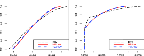
Figure 1: Left panel: $p=100$, $n=1\mbox{,}000$; right panel: $p=2\mbox{,}000$, $n=1\mbox{,}000$.

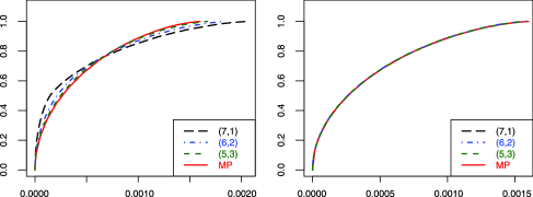
Figure 2: Comparisons, different values of piecewise constants ($a,b$) as shown in the legend, which are such that the targeting ICV matrix is the same; the red solid curve is the Marc̆enko–Pastur law (the LSD of $\Sigma^{\mathrm{RCV}^{0}}$). $p$ and $n$ are both taken to be $1\mbox{,}000$. Left panel: RCV; right panel: TVARCV.

We see from Figure 1 that:

• the ESDs of RCV matrices are very different from the LSD given by the Marc̆enko–Pastur law (the LSD of $\Sigma^{\mathrm{RCV}^{0}}$);

• the ESDs of TVARCV matrices follow the LSD given by the Marc̆enko–Pastur law very well, for both pairs of $p$ and $n$, even when $p$ is small compared with $n$.

In fact, the dependence of the ESD of RCV matrix on the time variability of covolatility process can be seen more clearly from Figure 2, where we consider the same design but different values for $\gamma_{t}$:

$$\gamma_{t}=\cases{a^{1/2}\times 10^{-2},&\quad$t\in[0,1/4)\cup[3/4,1]$,\cr b^{1/2}\times 10^{-2},&\quad$t\in[1/4,3/4)$,}\qquad\mbox{where }a+b=8.$$

We plot the ESDs of RCV and TVARCV matrices for the case when $p=n=1\mbox{,}000$, in the left and right panel, respectively. The curves’ corresponding parameters $(a,b)$ are reported in the legend. Note that since all pairs of $(a,b)$ have the same summation, in all cases the targeting ICV matrices are the same.

We see clearly from Figure 2 that, the ESDs of RCV matrices can be very different from each other even though the RCV matrices are estimating the same ICV matrix; while for TVARCV matrices, the ESDs are almost identical.

4.2 Design II, continuous paths

We illustrate in this subsection the case when the volatility processes have continuous sample paths. In particular, we assume that $\mathbf{X}_{t}$ satisfies (8) with

$$\gamma_{t}=\sqrt{0.0009+0.0008\cos(2\pi t)},\qquad t\in[0,1].$$

We see from Figure 3 similar phenomena as in Design I about the ESDs of RCV and TVARCV matrices for different pairs of $p$ and $n$.

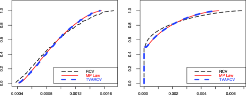
Figure 3: Left panel: $p=100$, $n=1\mbox{,}000$; right panel: $p=2\mbox{,}000$, $n=1\mbox{,}000$.

5 Conclusion and discussions

We have shown theoretically and via simulation studies that:

• the limiting spectral distribution (LSD) of RCV matrix depends not only on that of the ICV matrix, but also on the time-variability of covolatility process;

• in particular, even with the same targeting ICV matrix, the empirical spectral distribution (ESD) of RCV matrix can vary a lot, depending on how the underlying covolatility process evolves over time;

• for a class $\mathcal{C}$ of processes, our proposed estimator, the time-variation adjusted realized covariance (TVARCV) matrix, possesses the following desirable properties as an estimator of the ICV matrix: as long as the targeting ICV matrix is the same, the ESDs of TVARCV matrices estimated from processes with different covolatility paths will be close to each other, sharing a unique limit; moreover, the LSD of TVARCV matrix is related to that of the targeting ICV matrix through the same Marc̆enko–Pastur equation as in the sample covariance matrix case.

Furthermore, we establish a Marc̆enko–Pastur type theorem for weighted sample covariance matrices. For a class $\mathcal{C}$ of processes, we also establish a Marc̆enko–Pastur type theorem for RCV matrices, which explicitly demonstrates how the time-variability of the covolatility process affects the LSD of RCV matrix.

In practice, for given $p$ and $n$, based on the (observable) ESD of TVARCV matrix, one can use existing algorithms to obtain an estimate of the ESD of ICV matrix, which can then be applied to further applications such as portfolio allocation, risk management, etc.

References

- Admati and Pfleiderer (1988) {barticle}[author] \bauthor\bsnmAdmati, \bfnmAnat R.\binitsA. R. and \bauthor\bsnmPfleiderer, \bfnmPaul\binitsP. (\byear1988). \btitleA theory of intraday patterns: Volume and price variability. \bjournalRev. Financ. Stud. \bvolume1 \bpages3–40. \bptokimsref \endbibitem
- Andersen and Bollerslev (1997) {barticle}[author] \bauthor\bsnmAndersen, \bfnmTorben G.\binitsT. G. and \bauthor\bsnmBollerslev, \bfnmTim\binitsT. (\byear1997). \btitleIntraday periodicity and volatility persistence in financial markets. \bjournalJournal of Empirical Finance \bvolume4 \bpages115–158. \bptokimsref \endbibitem
- Andersen and Bollerslev (1998) {barticle}[author] \bauthor\bsnmAndersen, \bfnmTorben G.\binitsT. G. and \bauthor\bsnmBollerslev, \bfnmTim\binitsT. (\byear1998). \btitleDeutsche mark–dollar volatility: Intraday activity patterns, macroeconomic announcements, and longer run dependencies. \bjournalJ. Finance \bvolume53 \bpages219–265. \bptokimsref \endbibitem
- Andersen et al. (2001) {barticle}[mr] \bauthor\bsnmAndersen, \bfnmTorben G.\binitsT. G., \bauthor\bsnmBollerslev, \bfnmTim\binitsT., \bauthor\bsnmDiebold, \bfnmFrancis X.\binitsF. X. and \bauthor\bsnmLabys, \bfnmPaul\binitsP. (\byear2001). \btitleThe distribution of realized exchange rate volatility. \bjournalJ. Amer. Statist. Assoc. \bvolume96 \bpages42–55. \biddoi=10.1198/016214501750332965, issn=0162-1459, mr=1952727 \bptokimsref \endbibitem
- Bai (1999) {barticle}[mr] \bauthor\bsnmBai, \bfnmZ. D.\binitsZ. D. (\byear1999). \btitleMethodologies in spectral analysis of large-dimensional random matrices, a review. \bjournalStatist. Sinica \bvolume9 \bpages611–677. \bidissn=1017-0405, mr=1711663 \bptokimsref \endbibitem
- Bai, Chen and Yao (2010) {barticle}[mr] \bauthor\bsnmBai, \bfnmZhidong\binitsZ., \bauthor\bsnmChen, \bfnmJiaqi\binitsJ. and \bauthor\bsnmYao, \bfnmJianfeng\binitsJ. (\byear2010). \btitleOn estimation of the population spectral distribution from a high-dimensional sample covariance matrix. \bjournalAust. N. Z. J. Stat. \bvolume52 \bpages423–437. \biddoi=10.1111/j.1467-842X.2010.00590.x, issn=1369-1473, mr=2791528 \bptokimsref \endbibitem
- Bai, Liu and Wong (2009) {barticle}[mr] \bauthor\bsnmBai, \bfnmZhidong\binitsZ., \bauthor\bsnmLiu, \bfnmHuixia\binitsH. and \bauthor\bsnmWong, \bfnmWing-Keung\binitsW.-K. (\byear2009). \btitleEnhancement of the applicability of Markowitz’s portfolio optimization by utilizing random matrix theory. \bjournalMath. Finance \bvolume19 \bpages639–667. \biddoi=10.1111/j.1467-9965.2009.00383.x, issn=0960-1627, mr=2583523 \bptokimsref \endbibitem
- Bai and Silverstein (1998) {barticle}[mr] \bauthor\bsnmBai, \bfnmZ. D.\binitsZ. D. and \bauthor\bsnmSilverstein, \bfnmJack W.\binitsJ. W. (\byear1998). \btitleNo eigenvalues outside the support of the limiting spectral distribution of large-dimensional sample covariance matrices. \bjournalAnn. Probab. \bvolume26 \bpages316–345. \biddoi=10.1214/aop/1022855421, issn=0091-1798, mr=1617051 \bptokimsref \endbibitem
- Barndorff-Nielsen and Shephard (2004) {barticle}[mr] \bauthor\bsnmBarndorff-Nielsen, \bfnmOle E.\binitsO. E. and \bauthor\bsnmShephard, \bfnmNeil\binitsN. (\byear2004). \btitleEconometric analysis of realized covariation: High frequency based covariance, regression, and correlation in financial economics. \bjournalEconometrica \bvolume72 \bpages885–925. \biddoi=10.1111/j.1468-0262.2004.00515.x, issn=0012-9682, mr=2051439 \bptokimsref \endbibitem
- Barndorff-Nielsen et al. (2011) {barticle}[author] \bauthor\bsnmBarndorff-Nielsen, \bfnmOle E.\binitsO. E., \bauthor\bsnmHansen, \bfnmPeter Reinhard\binitsP. R., \bauthor\bsnmLunde, \bfnmAsger\binitsA. and \bauthor\bsnmShephard, \bfnmNeil\binitsN. (\byear2011). \btitleMultivariate realised kernels: Consistent positive semi-definite estimators of the covariation of equity prices with noise and non-synchronous trading. \bjournalJ. Econometrics \bvolume162 \bpages149–169. \bptokimsref \endbibitem
- El Karoui (2008) {barticle}[mr] \bauthor\bsnmEl Karoui, \bfnmNoureddine\binitsN. (\byear2008). \btitleSpectrum estimation for large dimensional covariance matrices using random matrix theory. \bjournalAnn. Statist. \bvolume36 \bpages2757–2790. \biddoi=10.1214/07-AOS581, issn=0090-5364, mr=2485012 \bptokimsref \endbibitem
- Fan, Li and Yu (2011) {bmisc}[author] \bauthor\bsnmFan, \bfnmJianqing\binitsJ., \bauthor\bsnmLi, \bfnmYingying\binitsY. and \bauthor\bsnmYu, \bfnmKe\binitsK. (\byear2011). \bhowpublishedVast volatility matrix estimation using high frequency data for portfolio selection. J. Amer. Statist. Assoc. To appear. \bptokimsref \endbibitem
- Geronimo and Hill (2003) {barticle}[mr] \bauthor\bsnmGeronimo, \bfnmJeffrey S.\binitsJ. S. and \bauthor\bsnmHill, \bfnmTheodore P.\binitsT. P. (\byear2003). \btitleNecessary and sufficient condition that the limit of Stieltjes transforms is a Stieltjes transform. \bjournalJ. Approx. Theory \bvolume121 \bpages54–60. \biddoi=10.1016/S0021-9045(02)00042-4, issn=0021-9045, mr=1962995 \bptokimsref \endbibitem
- Horn and Johnson (1990) {bbook}[mr] \bauthor\bsnmHorn, \bfnmRoger A.\binitsR. A. and \bauthor\bsnmJohnson, \bfnmCharles R.\binitsC. R. (\byear1990). \btitleMatrix Analysis. \bpublisherCambridge Univ. Press, \baddressCambridge. \bnoteCorrected reprint of the 1985 original. \bidmr=1084815 \bptokimsref \endbibitem
- Jacod and Protter (1998) {barticle}[mr] \bauthor\bsnmJacod, \bfnmJean\binitsJ. and \bauthor\bsnmProtter, \bfnmPhilip\binitsP. (\byear1998). \btitleAsymptotic error distributions for the Euler method for stochastic differential equations. \bjournalAnn. Probab. \bvolume26 \bpages267–307. \biddoi=10.1214/aop/1022855419, issn=0091-1798, mr=1617049 \bptokimsref \endbibitem
- Marčenko and Pastur (1967) {barticle}[mr] \bauthor\bsnmMarčenko, \bfnmV. A.\binitsV. A. and \bauthor\bsnmPastur, \bfnmL. A.\binitsL. A. (\byear1967). \btitleDistribution of eigenvalues in certain sets of random matrices. \bjournalMat. Sb. (N.S.) \bvolume72 \bpages507–536. \bidmr=0208649 \bptokimsref \endbibitem
- Markowitz (1952) {barticle}[author] \bauthor\bsnmMarkowitz, \bfnmHarry\binitsH. (\byear1952). \btitlePortfolio selection. \bjournalJ. Finance \bvolume7 \bpages77–91. \bptokimsref \endbibitem
- Markowitz (1959) {bbook}[mr] \bauthor\bsnmMarkowitz, \bfnmHarry M.\binitsH. M. (\byear1959). \btitlePortfolio Selection: Efficient Diversification of Investments. \bseriesCowles Foundation for Research in Economics at Yale University, Monograph \bvolume16. \bpublisherWiley, \baddressNew York. \bidmr=0103768 \bptokimsref \endbibitem
- Mestre (2008) {barticle}[mr] \bauthor\bsnmMestre, \bfnmXavier\binitsX. (\byear2008). \btitleImproved estimation of eigenvalues and eigenvectors of covariance matrices using their sample estimates. \bjournalIEEE Trans. Inform. Theory \bvolume54 \bpages5113–5129. \biddoi=10.1109/TIT.2008.929938, issn=0018-9448, mr=2589886 \bptokimsref \endbibitem
- Silverstein (1995) {barticle}[mr] \bauthor\bsnmSilverstein, \bfnmJack W.\binitsJ. W. (\byear1995). \btitleStrong convergence of the empirical distribution of eigenvalues of large-dimensional random matrices. \bjournalJ. Multivariate Anal. \bvolume55 \bpages331–339. \biddoi=10.1006/jmva.1995.1083, issn=0047-259X, mr=1370408 \bptokimsref \endbibitem
- Silverstein and Bai (1995) {barticle}[mr] \bauthor\bsnmSilverstein, \bfnmJack W.\binitsJ. W. and \bauthor\bsnmBai, \bfnmZ. D.\binitsZ. D. (\byear1995). \btitleOn the empirical distribution of eigenvalues of a class of large-dimensional random matrices. \bjournalJ. Multivariate Anal. \bvolume54 \bpages175–192. \biddoi=10.1006/jmva.1995.1051, issn=0047-259X, mr=1345534 \bptokimsref \endbibitem
- Silverstein and Choi (1995) {barticle}[mr] \bauthor\bsnmSilverstein, \bfnmJack W.\binitsJ. W. and \bauthor\bsnmChoi, \bfnmSang-Il\binitsS.-I. (\byear1995). \btitleAnalysis of the limiting spectral distribution of large-dimensional random matrices. \bjournalJ. Multivariate Anal. \bvolume54 \bpages295–309. \biddoi=10.1006/jmva.1995.1058, issn=0047-259X, mr=1345541 \bptokimsref \endbibitem
- Tao et al. (2011) {barticle}[auto:STB—2012/01/09—08:49:38] \bauthor\bsnmTao, \bfnmM.\binitsM., \bauthor\bsnmWang, \bfnmY.\binitsY., \bauthor\bsnmYao, \bfnmY.\binitsY. and \bauthor\bsnmZou, \bfnmJ.\binitsJ. (\byear2011). \btitleLarge volatility matrix inference via combining low-frequency and high-frequency approaches. \bjournalJ. Amer. Statist. Assoc. \bvolume106 \bpages1025–1040. \bptokimsref \endbibitem
- Wang and Zou (2010) {barticle}[mr] \bauthor\bsnmWang, \bfnmYazhen\binitsY. and \bauthor\bsnmZou, \bfnmJian\binitsJ. (\byear2010). \btitleVast volatility matrix estimation for high-frequency financial data. \bjournalAnn. Statist. \bvolume38 \bpages943–978. \biddoi=10.1214/09-AOS730, issn=0090-5364, mr=2604708 \bptokimsref \endbibitem
- Yin (1986) {barticle}[mr] \bauthor\bsnmYin, \bfnmY. Q.\binitsY. Q. (\byear1986). \btitleLimiting spectral distribution for a class of random matrices. \bjournalJ. Multivariate Anal. \bvolume20 \bpages50–68. \biddoi=10.1016/0047-259X(86)90019-9, issn=0047-259X, mr=0862241 \bptokimsref \endbibitem
- Zheng and Li (2011) {bmisc}[author] \bauthor\bsnmZheng, \bfnmXinghua\binitsX. and \bauthor\bsnmLi, \bfnmYingying\binitsY. (\byear2011). \bhowpublishedSupplement to “On the estimation of integrated covariance matrices of high dimensional diffusion processes.” DOI:10.1214/11-AOS939SUPP. \bptokimsref \endbibitem