Tol 2240–384 - a new low-metallicity AGN candidate

Abstract

Context. Active galactic nuclei (AGNs) have typically been discovered in massive galaxies of high metallicity.

Aims. We attempt to increase the number of AGN candidates in low metallicity galaxies. We present VLT/UVES and archival VLT/FORS1 spectroscopic and NTT/SUSI2 photometric observations of the low-metallicity emission-line galaxy Tol 2240–384 and perform a detailed study of its morphology, chemical composition, and emission-line profiles.

Methods. The profiles of emission lines in the UVES and FORS1 spectra are decomposed into several components with different kinematical properties by performing multicomponent fitting with Gaussians. We determine abundances of nitrogen, oxygen, neon, sulfur, chlorine, argon, and iron by analyzing the fluxes of narrow components of the emission lines using empirical methods. We verify with a photoionisation model that the physics of the narrow-line component gas is similar to that in common metal-poor galaxies.

Results. Image deconvolution reveals two high-surface brightness regions in Tol 2240–384 separated by 2.4 kpc. The brightest southwestern region is surrounded by intense ionised gas emission that strongly affects the observed $B-R$ colour on a spatial scale of $\sim$5 kpc. The profiles of the strong emission lines in the UVES spectrum are asymmetric and all these lines apart from H$\alpha$ and H$\beta$ can be fitted by two Gaussians of FWHM $\sim$ 75 – 92 km s^-1 separated by $\sim$ 80 km s^-1 implying that there are two regions of ionised gas emitting narrow lines. The oxygen abundances in both regions are equal within the errors and in the range 12+log O/H = 7.83 – 7.89. The shapes of the H$\alpha$ and H$\beta$ lines are more complex. In particular, the H$\alpha$ emission line consists of two broad components of FWHM $\sim$ 700 km s^-1 and 2300 km s^-1, in addition to narrow components of two regions revealed from profiles of other lines. This broad emission in H$\alpha$ and H$\beta$ associated with the high-excitation, brighter southwestern H ii region of the galaxy is also present in the archival low- and medium-resolution VLT/FORS1 spectra. The extraordinarily high luminosity of the broad H$\alpha$ line of 3 $\times$ 10⁴¹ erg s^-1 cannot be accounted for by massive stars at different stages of their evolution. The broad H$\alpha$ emission persists over a period of 7 years, which excludes supernovae as a powering mechanism of this emission. This emission most likely arises from an accretion disc around a black hole of mass $\sim$ 10⁷ $M_{\odot}$.

1 Introduction

Active galactic nuclei (AGNs) are understood to be powered by massive black holes at the centers of galaxies, accreting gas from their surroundings. They are usually found in massive, bulge-dominated galaxies and their gas metallicities are generally high (Storchi-Bergmann et al., 1998; Hamann et al., 2002; Ho, 2009). However, it remains unclear whether AGNs in low-metallicity low-mass galaxies do exist. Groves et al. (2006) and Barth et al. (2008) searched the Sloan Digital Sky Survey (SDSS) spectroscopic galaxy samples for low-mass Seyfert 2 galaxies. In particular, Groves et al. (2006) used a sample of 23 000 Seyfert 2 galaxies selected by Kauffmann et al. (2003) and found only $\sim$ 40 Seyfert 2 galaxies among them with masses lower than 10¹⁰ $M_{\odot}$. They demonstrated, however, that the metallicities of these AGNs are around solar or slightly subsolar. The same high metallicity range is found in the SDSS sample of 174 low-mass broad-line AGNs of Greene & Ho (2007). On the other hand, Izotov et al. (2007) and Izotov & Thuan (2008) demonstrated that broad-line AGNs with much lower metallicities probably exist, although they occupy a region in the diagnostic diagram differing from that of more metal-rich AGNs and are extremely rare. They identified four of these galaxies, which were found to have oxygen abundances 12 + log O/H in the range 7.36 – 7.99 on the basis of a systematic search for extremely metal-deficient emission-line dwarf galaxies in the SDSS Data Release 5 (DR5) database of 675 000 spectra. The absolute magnitudes of those four low-metallicity AGNs are typical of dwarf galaxies, their host galaxies have a compact structure, and their spectra resemble those of low-metallicity high-excitation H ii regions. Izotov et al. (2007) found that there is however a striking difference: the strong permitted emission lines, mainly the H$\alpha$ $\lambda$6563 line, show very prominent broad components characterised by properties unusual for dwarf galaxies: 1) their H$\alpha$ full widths at zero intensity (FWZI) vary from 102 to 158 Å, corresponding to expansion velocities between 2200 and 3500 km s^-1; 2) the broad H$\alpha$ luminosities $L_{br}$ are extraordinarily large, between 3$\times$10⁴¹ and 2$\times$10⁴² erg s^-1. This is higher than the range 10³⁷–10⁴⁰ erg s^-1 found by Izotov et al. (2007) for the other emission-line galaxies (ELGs) with broad-line emission. The ratio of H$\alpha$ flux in the broad component to that in the narrow component varies from 0.4 to 3.4, compared to 0.01–0.20 for the other galaxies; 3) the Balmer lines exhibit a very steep decrement, which is indicative of collisional excitation and the broad emission originating in very dense gas ($N_{e}$$>$10⁷ cm^-3).

To account for the broad-line emission in these four objects, Izotov et al. (2007) considered various physical mechanisms such as Wolf-Rayet (WR) stars, stellar winds from Ofp or luminous blue variable stars, single or multiple supernova (SN) remnants propagating in the interstellar medium, and SN bubbles. While these mechanisms may be able to produce $L_{br}$ $\sim$ 10³⁶ to 10⁴⁰ erg s^-1, they cannot generate yet higher luminosities, which are more likely associated with SN shocks or AGNs. Izotov et al. (2007) considered type IIn SNe because their H$\alpha$ luminosities are higher ($\sim$10³⁸–10⁴¹ erg s^-1) than those of the other SN types and they decrease less rapidly. Izotov & Thuan (2008) found no significant temporal evolution of broad H$\alpha$ in all four galaxies over a period of 3–7 years. Therefore, the IIn SNe mechanism may be excluded, leaving only the AGN mechanism capable of accounting for the high luminosity of the broad H$\alpha$ emission. However, we also have difficulty with this mechanism. In particular, all four galaxies are present in neither the ROSAT catalogue of the X-ray sources nor the NVSS catalogue of radio sources. High-ionisation emission lines such as He ii $\lambda$4686 or [Ne v] $\lambda$3426 are weak or not detected in optical spectra. Based on the observational evidence, Izotov & Thuan (2008) concluded that all four studied galaxies most likely belong to the very rare type of low-metallicity AGNs in which non-thermal ionising radiation is strongly diluted by the radiation of a young massive stellar population.

The fifth galaxy of this type, Tol 2240–384, was first spectroscopically studied by Terlevich et al. (1991) and Masegosa et al. (1994). However, in those low-resolution spectra, some important emission lines, such as [O ii] $\lambda$3727, [Ne iii] $\lambda$3868, and H$\alpha$ $\lambda$6563, are missing. This, in particular, precludes abundance determination and the detection of broad hydrogen emission. Kehrig et al. (2004, 2006) studied Tol 2240–384 spectroscopically, and Kehrig et al. (2006) derived the oxygen abundance of this galaxy, 12+logO/H = 7.77 $\pm$ 0.08. We note that no broad emission was reported by Terlevich et al. (1991), Masegosa et al. (1994), and Kehrig et al. (2006). In this paper, we present 8.2m Very Large Telescope (VLT) spectroscopic observations and 3.5 ESO New Technology Telescope (NTT) photometric observations of this emission-line galaxy. Its optical spectrum shows the very broad components of hydrogen emission lines and is similar to those found previously by Izotov et al. (2007) and Izotov & Thuan (2008) for the four other galaxies. We describe observations in Sect.2. The morphology of the galaxy is discussed in Sect.3 and its location in the emission-line diagnostic diagram is discussed in Sect.4. Element abundances are derived in Sect.5. The kinematics of the ionised gas from narrow emission lines is discussed in Sect.6. We discuss in Sect.7 the properties of the broad emission and derive the mass of the central black hole assuming an AGN mechanism for the origin of the broad line emission. Our conclusions are summarized in Sect.8.

Figure 1: Flux-calibrated VLT/UVES spectrum of Tol 2240–384, obtained on 23 August 2009, corrected for the redshift of $z$ = 0.07595 [ESO program 383.B-0271(A)] (upper spectrum). The lower spectrum is the upper spectrum downscaled by a factor of 100. The scale of the ordinate is that for the upper spectrum. Note the broad emission in the hydrogen line H$\alpha$ $\lambda$6563. No appreciable broad emission is detected in other strong permitted and forbidden lines, which is indicative of the rapid motions of relatively dense ionised gas with an electron number density $N_{e}$ $\geq$ 10⁷ cm^-3.

Figure 2: Flux-calibrated and redshift-corrected archival VLT/FORS1 medium-resolution (left) and low-resolution (right) spectra of Tol 2240–384 obtained on 12 September 2002 [ESO program 69.C-0203(A)] (upper spectra). The lower spectra are the upper spectra downscaled by a factor of 100. The scale of the ordinate is that for the upper spectra. Note the strong broad emission in the hydrogen line H$\alpha$ $\lambda$6563 and much weaker broad emission in the hydrogen line H$\beta$ $\lambda$4861. No appreciable broad emission is detected in strong forbidden lines.

2 Observations

2.1 Spectroscopy

A new optical spectrum of Tol 2240–384 was obtained using the 8.2 m Very Large Telescope (VLT) on 2009 August 23 [ESO program 383.B-0271(A)]. The observations were performed using the UVES echelle spectrograph mounted at the UT2. We used the gratings CD#1 with the central wavelength 3460Å, CD#2 with the central wavelength 4370Å, CD#3 with the central wavelength 5800Å, and CD#4 with the central wavelength 8600Å. The slits were used with lengths of 8″ and 12″ for the blue (CD#1 and CD#2) and red (CD#3 and CD#4) parts of the spectra, respectively, and with a width of 3″. The angular scale along the slit was 0$\aas@@fstack{\prime\prime}$246 and 0$\aas@@fstack{\prime\prime}$182 for the blue and red arms, respectively. The above instrumental set-up resulted in a spectral range $\sim$3000 – 10 200Å over 131 orders and a resolving power $\lambda$/$\Delta$$\lambda$ of $\sim$ 80 000. The total exposure time was 2960s for gratings CD#1 and CD#3, and 2970s for gratings CD#2 and CD#4, divided into 2 equal subexposures. Observations were performed at airmass $\sim$1.2 with gratings CD#1 and CD#3 and $\sim$1.5 with gratings CD#2 and CD#4. The seeing was $\sim$2″. The Kitt Peak IRS spectroscopic standard star Feige 110 was observed for flux calibration. Spectra of thorium (Th) comparison arcs were obtained for wavelength calibration.

We supplemented the UVES observations with ESO archival data of Tol 2240–384 (ESO program 69.C-0203(A)). These observations were obtained on 12 September, 2002 with the FORS1 spectrograph mounted at the UT3 of the 8.2m ESO VLT. The observing conditions were photometric throughout the night.

Two sets of spectra were obtained. Low-resolution spectra were obtained with a grism 300V ($\lambda$$\lambda$$\sim$3850–7500) and a blocking filter GG 375. The grisms 600B ($\lambda$$\lambda$$\sim$3560–5970) and 600R ($\lambda$$\lambda$$\sim$5330–7480) for the blue and red wavelength ranges were used in the medium-resolution observations. To avoid second-order contamination, the red part of the spectrum was obtained with the blocking filter GG 435.

A long ($\sim$418″) slit with a width of 0$\aas@@fstack{\prime\prime}$51 was used. The spatial scale along the slit was 0$\aas@@fstack{\prime\prime}$2 pixel^-1 and the resolving power $\lambda$/$\Delta$$\lambda$ = 300 in the low-resolution mode and $\lambda$/$\Delta$$\lambda$ = 780 and 1160 in a medium-resolution mode for the 600B and 600R grisms, respectively. The spectra were obtained at airmass $\sim$ 1.2 – 1.4. The seeing was $\sim$ 1$\aas@@fstack{\prime\prime}$2 during the low-resolution observations, 1″ during the medium-resolution observations in the blue range, and 1$\aas@@fstack{\prime\prime}$5 during the medium-resolution observations in the red range. The total integration time for the low-resolution observations was 360s (3 $\times$ 120s). The longer exposures were taken for the medium-resolution observations and consisted of 2160s (3 $\times$ 720s) and 1800s (3 $\times$ 600s) for the blue and red parts, respectively.

The two-dimensional spectra were bias subtracted and flat-field corrected using IRAF. We then used the IRAF software routines IDENTIFY, REIDENTIFY, FITCOORD, and TRANSFORM to perform wavelength calibration and correct for distortion and tilt for each frame. Night sky subtraction was performed using the routine BACKGROUND. The level of night sky emission was determined from the closest regions to the galaxy that are free of galaxian stellar and nebular line emission, as well as of emission from foreground and background sources. The one-dimensional spectra were then extracted from the two-dimensional frame using the APALL routine. We adopted extraction apertures of 3″$\times$ 4″ for the UVES spectrum and 0$\aas@@fstack{\prime\prime}$51 $\times$ 4″ for FORS1 spectra. Before extraction, the two distinct two-dimensional UVES spectra, the three distinct two-dimensional low-resolution FORS1 spectra, and the three distinct two-dimensional medium-resolution FORS1 spectra were carefully aligned with the routine ROTATE using the spatial locations of the brightest parts in each spectrum, so that the spectra were extracted at the same positions in all subexposures. We then summed the individual spectra from each subexposure after manual removal of the cosmic ray hits.

The resulting UVES spectrum of Tol 2240–384 is shown in Fig. 1. A strong broad H$\alpha$ emission line is present in the spectrum, very similar to the one seen in the spectra of the four low-metallicity AGN candidates discussed by Izotov et al. (2007) and Izotov & Thuan (2008). The broad component in the H$\beta$ emission line is much weaker, suggesting a steep Balmer decrement and hence that the broad emission originates in a very dense gas.

The extracted medium-resolution and low-resolution spectra of Tol 2240–384 are shown in Figs. 2a and 2b, respectively. As in the UVES spectrum, a broad H$\alpha$ emission line is detected. The signal-to-noise ratio of the FORS1 spectra is higher than that of the UVES spectrum because of the lower spectral resolution of the former. This allows us to detect broad components of the H$\gamma$ and H$\beta$ emission lines. As in the UVES data, the broad H$\beta$ emission line in the FORS1 spectra is much weaker than the broad H$\alpha$ emission line.

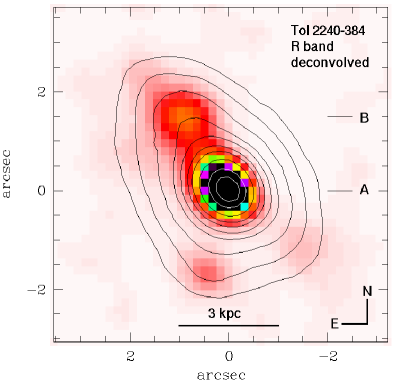
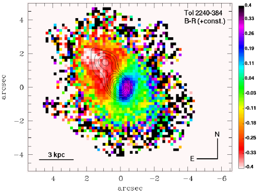
Figure 3: left: Deconvolved $R$ image of Tol 2240–384 revealing two high-surface brightness regions separated by 1$\aas@@fstack{\prime\prime}$6 and differing in their luminosities by a factor $\sim$10. The overlaid contours illustrate the morphology of the galaxy prior to deconvolution, at a resolution of 0$\aas@@fstack{\prime\prime}$9 (FWHM). right: Uncalibrated $B-R$ map of Tol 2240–384. Note the presence of a strong colour contrast between the southwestern and northeastern half of the galaxy. The contours correspond to the deconvolved $R$ image.

2.2 Photometry

To gain additional insight into the morphological and photometric properties of Tol 2240–384, we study archival [ESO program 71.B-0509(A)] images for this system in the Bessel filters $U$ (3 $\times$ 200s), $B$ (3 $\times$ 400s), and $R$ (3 $\times$ 300s). These data were taken with the SUSI2 camera (0$\aas@@fstack{\prime\prime}$161 pixel^-1) attached to the 3.5m ESO NTT in seeing conditions of $\approx$1″ in $U$ and $B$, and 0$\aas@@fstack{\prime\prime}$9 in $R$. Image reduction and analysis was carried out using MIDAS and additional routines developed by ourselves. From the available calibration exposures, it was not possible to establish photometric zero points with an accuracy better than $\sim$ 0.2 mag. In the following, we therefore restrict ourselves to discussing the morphology and the relative colour distribution of Tol 2240–384. From the approximate apparent $B$ band magnitude of 16 mag that we obtained for this system, and assuming a distance of 310 Mpc from the NASA/IPAC Extragalactic Database (NED) (corrected for Virgocentric infall and based on $H_{0}$=73 km s^-1 Mpc^-1), we estimate its absolute magnitude to be $\sim$ –21 $B$ mag. This is 2 – 4 mag brighter than the absolute SDSS $g$ magnitudes of four low-metallicity AGNs studied by Izotov & Thuan (2008).

3 Morphology of Tol 2240-384

The morphology of Tol 2240–384, as inferred from the combined $R$ band exposure, is illustrated with the contours in Fig. 3 (left). It can be seen that the galaxy is unresolved and shows merely a slight NE–SW elongation on a projected scale of 7$\times$5 kpc. On the same panel, we display the $R$ band image after Lucy deconvolution (Lucy, 1974), which contains two main high-surface brightness regions, separated by 1$\aas@@fstack{\prime\prime}$6 (2.4 kpc). The southwestern region (labelled A) coincides with the surface brightness maximum of the galaxy and is about ten times more luminous than the northeastern region B. This result was checked and confirmed using a flux-conserving unsharp masking technique (Papaderos et al., 1998).

In Fig. 3 (right), we show the uncalibrated $B-R$ map of Tol 2240–384 with the overlaid contours depicting the morphology of the deconvolved $R$ image. The colour map reveals a strong colour contrast of nearly 0.8 mag between the SW and NE half of the galaxy with a relatively sharp transition between these two regions at the periphery of knot A. Knots A and B are located respectively within the red ($\ga-0.1$ mag) (shown by purple, blue, and green colours in Fig. 3 (right)) and blue ($\la-0.1$ mag) (shown by white and red colours in Fig. 3 (right)) halves of Tol 2240–384. They do not, however, spatially coincide with the locations where the extremal colour indices are observed. More specifically, the reddest and bluest features on the colour map are offset by between 0$\aas@@fstack{\prime\prime}$5 and 0$\aas@@fstack{\prime\prime}$9 from regions A and B. The extended, almost uniformly red colour pattern in the SW half of Tol 2240–384 is indicative of intense ionised gas emission surrounding the brightest region A on spatial scales of $\sim$5 kpc. Strong H$\alpha$ emission, with an equivalent width of 1300 Å in the UVES spectrum, registered within the $R$ band transmission curve, can readily shift optical colours by more than 0.5 mag. We note that extreme contamination of optical colours by extended and intense nebular line emission several kpc away from young stellar clusters has been observed in several low-mass starburst galaxies (e.g., Izotov et al., 1997; Papaderos et al., 1998, 2002). As we discuss below, intense H$\alpha$ emission, including a strong broad component, is associated with region A. In contrast, no appreciable ionised gas emission is present in the NE part of the galaxy, indicating that the blue $B-R$ colour in region B and its surroundings is mainly due to stellar emission.

In Fig. 4, we show the surface brightness profiles (SBPs) of Tol 2240–384 in $U$ (squares), $B$ (dots) and $R$ (open circles). The SBPs were computed with the method iv in Papaderos et al. (2002) and shifted vertically to an equal central surface brightness. The point spread function (PSF) in the $B$, derived from two well-exposed nearby stars in the field is included for comparison. We note that the slight bump in the SBPs at a photometric radius $R^{\star}\approx$1$\aas@@fstack{\prime\prime}$6 reflects the luminosity contribution of the fainter knot B. In agreement with the evidence from the deconvolved $R$ band image (Fig. 3), the surface photometry does not support the existence of a bulge component in Tol 2240–384. It can be seen that all SBPs have an exponential slope in their outer parts. This component, reflecting the emission from the host galaxy of Tol 2240–384, contains approximately 50% of the total luminosity of the galaxy. The effective radius of 1.2 kpc determined for Tol 2240–384 is a factor of between 2 and 3 larger than typical values for blue compact dwarf (BCD) galaxies (cf. Papaderos et al., 2006). This is also the case for the exponential scale length $\alpha\approx 1$ kpc, derived from a linear fit to the $B$ band SBP for $R^{\star}\geq$1$\aas@@fstack{\prime\prime}$8.

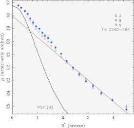
Figure 4: Surface brightness profiles (SBPs) of Tol 2240–384 in $U$, $B$, and $R$ computed with method iv in Papaderos et al. (2002). The point spread function (PSF) in the $B$ band, derived from two well-exposed nearby stars in the field of view, is shown with the gray curve. The straight line shows a linear fit to the host galaxy of Tol 2240–384 for radii $R^{\star}\geq$1$\aas@@fstack{\prime\prime}$8.

Table 1: Extinction-corrected narrow emission-line fluxes

	UVES				FORS
Line	total	blue	red		medium	low
3188 He i	3.11$\pm$0.41	…	…		…	…
3727 [O ii]	86.95$\pm$1.45	93.45$\pm$2.13	69.49$\pm$4.65		43.91$\pm$0.74	64.03$\pm$1.31
3750 H12	3.07$\pm$0.49	…	…		3.11$\pm$0.21	4.59$\pm$0.83
3771 H11	3.34$\pm$0.60	…	…		3.61$\pm$0.19	5.57$\pm$0.62
3797 H10	5.26$\pm$0.55	…	…		4.24$\pm$0.18	5.99$\pm$0.59
3820 He i	…	…	…		0.71$\pm$0.07	1.63$\pm$0.29
3835 H9	7.10$\pm$0.05	…	…		5.48$\pm$0.19	7.91$\pm$0.57
3869 [Ne iii]	53.05$\pm$0.86	51.50$\pm$0.89	55.02$\pm$1.36		32.69$\pm$0.55	43.18$\pm$0.87
3889 He i + H8	16.70$\pm$0.72	…	…		11.64$\pm$0.25	15.53$\pm$0.61
3968 [Ne iii] + H7	34.24$\pm$0.76	…	…		21.62$\pm$0.38	29.49$\pm$0.71
4026 He i	2.21$\pm$0.23	…	…		1.16$\pm$0.07	1.85$\pm$0.24
4069 [S ii]	…	…	…		0.79$\pm$0.06	0.76$\pm$0.16
4076 [S ii]	…	…	…		0.28$\pm$0.05	…
4101 H$\delta$	27.37$\pm$0.66	27.35$\pm$0.88	28.91$\pm$1.60		18.26$\pm$0.32	23.34$\pm$0.61
4227 [Fe v]	…	…	…		2.02$\pm$0.56	…
4340 H$\gamma$	47.18$\pm$0.87	47.94$\pm$0.90	50.30$\pm$1.40		37.70$\pm$0.59	42.98$\pm$0.81
4363 [O iii]	14.73$\pm$0.31	14.63$\pm$1.09	14.51$\pm$1.67		11.92$\pm$0.20	14.87$\pm$0.32
4388 He i	…	…	…		0.36$\pm$0.04	…
4471 He i	4.46$\pm$0.16	4.16$\pm$0.42	4.20$\pm$0.95		3.70$\pm$0.08	4.03$\pm$0.17
4658 [Fe iii]	0.85$\pm$0.09	…	…		0.63$\pm$0.05	…
4686 He ii	0.93$\pm$0.09	…	…		1.38$\pm$0.06	1.76$\pm$0.15
4711 [Ar iv] + He i	2.52$\pm$0.29	…	…		2.07$\pm$0.06	2.49$\pm$0.15
4740 [Ar iv]	1.70$\pm$0.09	…	…		1.40$\pm$0.05	1.52$\pm$0.15
4861 H$\beta$	100.00$\pm$1.51	100.00$\pm$1.53	100.00$\pm$1.85		100.00$\pm$1.49	100.00$\pm$1.60
4921 He i	1.36$\pm$0.11	…	…		0.90$\pm$0.04	1.06$\pm$0.10
4959 [O iii]	222.99$\pm$3.22	217.93$\pm$3.16	231.89$\pm$3.58		218.33$\pm$3.24	213.39$\pm$3.29
4988 [Fe iii]	0.85$\pm$0.07	…	…		0.75$\pm$0.06	…
5007 [O iii]	663.85$\pm$9.54	647.74$\pm$9.35	704.02$\pm$9.99		663.42$\pm$9.81	644.11$\pm$9.83
5016 He i	2.42$\pm$0.11	…	…		…	…
5200 [N i]	0.60$\pm$0.09	…	…		…	…
5518 [Cl iii]	0.53$\pm$0.05	…	…		0.32$\pm$0.03	…
5755 [N ii]	0.48$\pm$0.13	…	…		0.38$\pm$0.05	0.48$\pm$0.08
5876 He i	13.76$\pm$0.23	13.83$\pm$0.29	13.96$\pm$0.76		12.51$\pm$0.22	12.99$\pm$0.25
6300 [O i]	2.58$\pm$0.06	…	…		2.01$\pm$0.06	2.13$\pm$0.08
6312 [S iii]	1.19$\pm$0.04	…	…		0.88$\pm$0.04	0.87$\pm$0.07
6364 [O i]	0.78$\pm$0.04	…	…		0.62$\pm$0.04	0.72$\pm$0.07
6548 [N ii]	2.09$\pm$0.06	…	…		…	…
6563 H$\alpha$	279.49$\pm$4.36	279.38$\pm$4.38	279.85$\pm$4.65		284.13$\pm$4.56	282.54$\pm$4.69
6583 [N ii]	6.08$\pm$0.10	…	…		5.68$\pm$0.12	5.01$\pm$0.14
6678 He i	3.12$\pm$0.07	…	…		2.77$\pm$0.07	2.51$\pm$0.09
6716 [S ii]	5.67$\pm$0.12	…	…		4.10$\pm$0.09	3.75$\pm$0.10
6731 [S ii]	4.41$\pm$0.08	…	…		3.56$\pm$0.08	3.05$\pm$0.09
7065 He i	1.45$\pm$0.05	…	…		…	4.60$\pm$0.12
7136 [Ar iii]	4.13$\pm$0.12	…	…		…	2.41$\pm$0.09
7281 He i	0.81$\pm$0.04	…	…		…	…
7320 [O ii]	2.40$\pm$0.09	…	…		…	…
7330 [O ii]	1.78$\pm$0.06	…	…		…	…
7751 [Ar iii]	0.81$\pm$0.04	…	…		…	…
8446 O i	1.02$\pm$0.04	…	…		…	…
8467 P17	0.39$\pm$0.02	…	…		…	…
8502 P16	0.50$\pm$0.03	…	…		…	…
8545 P15	0.44$\pm$0.03	…	…		…	…
8598 P14	0.70$\pm$0.03	…	…		…	…
8750 P12	1.21$\pm$0.04	…	…		…	…
8863 P11	1.60$\pm$0.05	…	…		…	…
9015 P10	2.03$\pm$0.05	…	…		…	…
9069 [S iii]	8.10$\pm$0.20	…	…		…	…
$C$(H$\beta$)	0.280	0.290	0.195		0.830	0.815
EW(H$\beta$)a	167	112	46		284	274
$F$(H$\beta$)b	234	157	65		80	73
EW(abs)a	0.2	0.3	0.1		5.2	5.6
a in Å.
b in units 10-16 erg s-1 cm-2.

Table 2: Physical conditions and element abundances

	UVES				FORS
Property	total	blue	red		medium	low
$T_{e}$(O iii), K	15980$\pm$190	16110$\pm$590	15470$\pm$840		14540$\pm$130	15780$\pm$200
$T_{e}$(O ii), K	14860$\pm$160	14930$\pm$500	14560$\pm$720		13960$\pm$120	14740$\pm$170
$T_{e}$(S iii), K	14960$\pm$150	15070$\pm$490	15010$\pm$700		14250$\pm$110	14800$\pm$170
$N_{e}$(O ii), cm-3	300$\pm$50	350$\pm$50	150$\pm$140		100$\pm$50	…
$N_{e}$(S ii), cm-3	140$\pm$40	…	…		320$\pm$60	210$\pm$70
O+/H+, ($\times$105)	0.82$\pm$0.03	0.86$\pm$0.08	0.69$\pm$0.10		0.52$\pm$0.02	0.63$\pm$0.02
O2+/H+, ($\times$105)	6.26$\pm$0.20	5.99$\pm$0.55	7.15$\pm$0.99		7.87$\pm$0.21	6.24$\pm$0.21
O3+/H+, ($\times$106)	0.59$\pm$0.06	…	…		1.27$\pm$0.07	1.20$\pm$0.11
O/H, ($\times$105)	7.14$\pm$0.20	6.85$\pm$0.56	7.78$\pm$1.00		8.52$\pm$0.21	6.99$\pm$0.21
12+log O/H	7.85$\pm$0.01	7.84$\pm$0.04	7.89$\pm$0.06		7.93$\pm$0.01	7.84$\pm$0.01
N+/H+, ($\times$106)	0.46$\pm$0.01	…	…		0.49$\pm$0.01	0.38$\pm$0.01
$ICF$(N)a	8.20	…	…		15.1	10.4
N/H, ($\times$106)	3.74$\pm$0.09	…	…		7.33$\pm$0.18	3.99$\pm$0.13
log N/O	–1.28$\pm$0.02	…	…		–1.07$\pm$0.02	–1.24$\pm$0.02
Ne2+/H+, ($\times$105)	1.19$\pm$0.04	1.13$\pm$0.11	1.35$\pm$0.19		0.96$\pm$0.03	1.00$\pm$0.04
$ICF$(Ne)a	1.04	1.04	1.03		1.03	1.04
Ne/H, ($\times$105)	1.23$\pm$0.05	1.17$\pm$0.12	1.39$\pm$0.21		0.99$\pm$0.03	1.04$\pm$0.04
log Ne/O	–0.76$\pm$0.02	–0.77$\pm$0.06	–0.75$\pm$0.09		–0.94$\pm$0.02	–0.83$\pm$0.02
S+/H+, ($\times$106)	0.10$\pm$0.01	…	…		0.09$\pm$0.01	0.07$\pm$0.01
S2+/H+, ($\times$106)	0.62$\pm$0.03	…	…		0.53$\pm$0.03	0.47$\pm$0.04
$ICF$(S)a	1.87	…	…		3.02	2.24
S/H, ($\times$106)	1.34$\pm$0.05	…	…		1.87$\pm$0.08	1.20$\pm$0.09
log S/O	–1.73$\pm$0.02	…	…		–1.66$\pm$0.02	–1.76$\pm$0.03
Cl2+/H+, ($\times$108)	2.43$\pm$0.19	…	…		1.65$\pm$0.13	…
$ICF$(Cl)a	1.28	…	…		1.64	…
Cl/H, ($\times$108)	3.12$\pm$0.24	…	…		2.71$\pm$0.21	…
log Cl/O	–3.36$\pm$0.04	…	…		–3.50$\pm$0.03	…
Ar2+/H+, ($\times$107)	1.67$\pm$0.05	…	…		…	0.99$\pm$0.04
Ar3+/H+, ($\times$107)	…	…	…		1.54$\pm$0.07	1.35$\pm$0.14
$ICF$(Ar)a	1.80	…	…		…	2.16
Ar/H, ($\times$107)	2.99$\pm$0.10	…	…		…	2.14$\pm$0.31
log Ar/O	–2.38$\pm$0.02	…	…		…	–2.51$\pm$0.06
Fe2+/H+, ($\times$106)(4658)	0.17$\pm$0.02	…	…		0.14$\pm$0.01	…
$ICF$(Fe)	12.0	…	…		22.8	…
Fe/H, ($\times$106)(4658)	1.97$\pm$0.20	…	…		3.27$\pm$0.26	…
log Fe/O (4658)	–1.22$\pm$0.05	…	…		–1.00$\pm$0.03	…
Fe2+/H+, ($\times$106)(4988)	…	…	…		0.17$\pm$0.01	…
$ICF$(Fe)a	…	…	…		22.8	…
Fe/H, ($\times$106)(4988)	…	…	…		3.88$\pm$0.32	…
log Fe/O (4988)	…	…	…		–0.92$\pm$0.04	…

^a Ionisation correction factor.

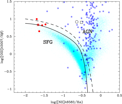
Figure 5: The Baldwin-Phillips-Terlevich (BPT) diagram (Baldwin et al., 1981) for narrow emission lines. Plotted are the $\sim$100 000 ELGs from SDSS DR7 (cloud of dots), the SDSS sample of broad-line AGNs with low-mass black holes of Greene & Ho (2007) (asterisks), the low-luminosity broad-line AGNs NGC 4395 (open circle, Kraemer et al., 1999) and Pox 52 (open square, Barth et al., 2004), the four low-metallicity AGNs from Izotov & Thuan (2008) (filled circles) and Tol 2240–384 (star). The dashed line by Kauffmann et al. (2003) and the solid line by Stasińska et al. (2006) separate star-forming galaxies (SFG) from active galactic nuclei (AGN).

Figure 6: Decomposition of strong emission line profiles into two Gaussian components in the UVES spectrum of Tol 2240–384 for: a) [O ii] $\lambda$3726 and $\lambda$3729, b) [O iii] $\lambda$4363, c) H$\beta$ $\lambda$4861 and d) [O iii] $\lambda$5007. Observational data are shown by solid lines and fits by dotted lines.

Figure 7: Decomposition of the H$\alpha$ $\lambda$6563 emission line profile into four Gaussian components. Two broad components of the H$\alpha$ emission line are shown by dashed lines, while two narrow components of H$\alpha$ and fits by single Gaussians for the [N ii] $\lambda$6548 and $\lambda$6583 emission lines are shown by solid lines.

Figure 8: The dependence of the theoretical H$\alpha$-to-H$\beta$ emission line flux ratio $I$(H$\alpha$)/$I$(H$\beta$) on the electron number density $N_{e}$ calculated with the CLOUDY photoionisation models for three values of the ionisation parameter log $U$ = –2 (thick solid line), log $U$ = –1 and log $U$ = –3 (thin solid lines) (Ferland, 1996; Ferland et al., 1998). For the ionising radiation, the power law spectral energy distribution $f_{\nu}$ $\propto$ $\nu^{\alpha}$ for $\alpha$ = –1 is chosen. An oxygen abundance of 12+logO/H = 7.6 is adopted for the gas. The dash-dotted line is the extinction-corrected H$\alpha$-to-H$\beta$ flux ratio measured in the UVES spectrum adopting $C$(H$\beta$) = 0.28, and the dashed line is the extinction-corrected H$\alpha$-to-H$\beta$ flux ratio measured in the medium-resolution FORS1 spectrum adopting the extinction coefficient $C$(H$\beta$) = 0.83. The range of possible electron number densities in the region of broad emission is shown by two vertical dotted lines assuming an ionising radiation field with log $U$ = –2.

4 Location in the emission-line diagnostic diagram

Figure 5 shows the position of Tol 2240–384 (represented by a star) in the classical [O iii] $\lambda$5007/H$\beta$ vs. [N ii] $\lambda$6583/H$\alpha$ diagram (Baldwin et al., 1981, hereafter BPT), in addition to other objects shown for comparison. The four objects from Izotov & Thuan (2008) are represented by filled circles and lie in the same region. The asterisks represent the broad-line AGNs with low black hole masses from Greene & Ho (2007). The two low-luminosity broad-line AGNs NGC 4395 and Pox 52 (Kraemer et al., 1999; Barth et al., 2004) are represented by an open circle and an open square, respectively. For reference, the cyan dots represent all the galaxies from the SDSS DR7 with flux errors smaller than 10% for each of the four emission lines, H$\beta$, [O iii] $\lambda$5007, H$\alpha$ and [N ii] $\lambda$6583. The emission line fluxes were measured using the technique developed by Tremonti et al. (2004) and were taken from the SDSS website. These galaxies are distributed into two wings, the left one interpreted as star-forming galaxies and the right one containing AGN hosts. The dashed line represents the empirical divisory line between star-forming galaxies and AGNs drawn by Kauffmann et al. (2003), while the continuous line represents the upper limit for pure star-forming galaxies from Stasińska et al. (2006). One can see that Tol 2240–384, as well as the four objects from Izotov & Thuan (2008) lie in the low metallicity part of what is usually considered as the region of star-forming galaxies. However, it has been shown by Stasińska et al. (2006) that an AGN hosted by a low metallicity galaxy would be difficult to distinguish in this diagram, even if the active nucleus contributed significantly to the emission lines (which is not the case in Tol 2240–384, as discussed later in this paper). The active galaxies from the Greene & Ho (2007) sample occupy a different zone in the BPT diagram, closer to the “AGN wing”, probably because their metallicities are higher than that of Tol 2240–384 and the four galaxies from Izotov & Thuan (2008), but lower than those of the bulk of AGN hosts.

5 Element abundances

5.1 Empirical analysis

We derived element abundances from the narrow emission-line fluxes, using a classical empirical method. Thanks to the high spectral resolution, the narrow emission lines in the UVES spectrum are resolved and found to have an asymmetric shape, implying the presence of two kinematically distinct emission-line regions in the SW part of the galaxy (Fig. 6). On the other hand, these lines are not resolved in the FORS1 spectra due to insufficient spectral resolution and have therefore the full widths at half maximum (FWHM) corresponding to the instrumental ones. Therefore, in the case of the UVES spectrum, the narrow emission lines were deblended and element abundances were derived from the emission line fluxes for every emitting region. To improve the accuracy of the abundance determination, we also derived element abundances for the total emission-line fluxes, including both blueshifted and redshifted components of the emission lines. The fluxes in all spectra were measured using Gaussian fitting with the IRAF SPLOT routine. They were corrected for both extinction, using the reddening curve of Whitford (1958), and underlying hydrogen stellar absorption, derived simultaneously by an iterative procedure described by Izotov et al. (1994) and using the observed decrements of the narrow hydrogen Balmer lines. The extinction coefficient $C$(H$\beta$) and equivalent width of hydrogen absorption lines EW(abs) are derived in such a way to obtain the closest agreement between the extinction-corrected and theoretical recombination hydrogen emission-line fluxes normalised to the H$\beta$ flux. It is assumed that EW(abs) is the same for all hydrogen lines. This assumption is justified by the evolutionary stellar population synthesis models of González Delgado et al. (2005).

The extinction-corrected total fluxes 100$\times$$I$($\lambda$)/$I$(H$\beta$) of the narrow lines from the UVES spectrum as well as fluxes of the blueshifted and redshifted components, and the extinction coefficient $C$(H$\beta$), the equivalent width of the H$\beta$ emission line EW(H$\beta$), the H$\beta$ observed flux $F$(H$\beta$), and the equivalent width of the underlying hydrogen absorption lines EW(abs) are given in Table 1. We note that total fluxes of hydrogen emission lines corrected for extinction and underlying hydrogen absorption (column 2 in Table 1) are very close to the theoretical recombination values of Hummer & Storey (1987) suggesting that the extinction coefficient $C$(H$\beta$) is reliably derived. We obtained EW(abs) of $\sim$ 0.2Å, which is much smaller than the equivalent widths of hydrogen emission lines, implying that the effect of underlying absorption on the emission line fluxes is very small, $\sim$ 2 percent for H9 $\lambda$3835 and much lower for stronger lines. In Table 1, we also show the emission-line fluxes and other parameters for the medium- and low-resolution FORS1 spectra. We note that the extinction coefficient $C$(H$\beta$) (Table 1) derived from the FORS1 spectra is significantly higher than that derived from the UVES spectrum. This difference is probably caused by the FORS1 spectra being obtained at the relatively high airmass of $\sim$ 1.2 – 1.4 with the narrow 0$\aas@@fstack{\prime\prime}$51 slit. Therefore, these spectra are affected by atmospheric refraction. This effect is seen by comparing the continuum slopes of the UVES and FORS1 spectra (Figs. 1 and 2), respectively. The continuum in the UVES spectrum is blue, while it is reddish in the FORS1 spectra. This effect is somewhat larger for the medium-resolution spectrum. We conclude that the FORS1 data are somewhat uncertain for the analysis of physical conditions and the abundance determination.

Table 3: Comparison of photoionisation models with observations

Line	observed	model M1	model M2
3727 [O ii]	86.95$\pm$1.45	86.58	86.21
3869 [Ne iii]	53.05$\pm$0.86	53.30	53.34
4363 [O iii]	14.73$\pm$0.31	14.55	14.67
4471 He i	4.46$\pm$0.16	5.10	5.00
4658 [Fe iii]	0.85$\pm$0.09	0.86	0.85
4686 He ii	0.93$\pm$0.09	0.93	0.93
4711 [Ar iv]	2.05$\pm$0.29	2.76	2.09
4740 [Ar iv]	1.70$\pm$0.09	2.07	1.56
4861 H$\beta$	100.00$\pm$1.51	100	100
5007 [O iii]	663.85$\pm$9.54	663.46	663.48
5755 [N ii]	0.48$\pm$0.13	0.15	0.14
5876 He i	13.76$\pm$0.23	13.26	13.14
6300 [O i]	2.58$\pm$0.06	1.32	1.79
6312 [S iii]	1.19$\pm$0.04	1.05	0.83
6563 H$\alpha$	279.49$\pm$4.36	281.13	283.11
6583 [N ii]	6.08$\pm$0.10	6.11	6.07
6716 [S ii]	5.67$\pm$0.12	5.68	6.54
6731 [S ii]	4.41$\pm$0.08	4.41	5.19
7136 [Ar iii]	4.13$\pm$0.12	2.52	2.13
7320 [O ii] +	4.18$\pm$0.10	3.03	2.90
9069 [S iii]	8.10$\pm$0.20	7.88	6.86
$F_{\rm corr}$(H$\beta$)a	446	442	464
a in units 10-16 erg s-1 cm-2.

The physical conditions, and the ionic and total heavy element abundances in the H ii regions of Tol 2240–384 were derived following Izotov et al. (2006) (Table 2). In particular for the O²⁺, Ne²⁺, and Ar³⁺, we adopt the temperature $T_{e}$(O iii) directly derived from the [O iii] $\lambda$4363/($\lambda$4959 + $\lambda$5007) emission-line ratio. The electron temperatures $T_{e}$(O ii) and $T_{e}$(S iii) were derived from the empirical relations by Izotov et al. (2006). We used $T_{e}$(O ii) for the calculation of O⁺, N⁺, S⁺, and Fe²⁺ abundances and $T_{e}$(S iii) for the calculation of S²⁺, Cl²⁺, and Ar²⁺ abundances. The electron number densities $N_{e}$(O ii) and $N_{e}$(S ii) were obtained from the [O ii] $\lambda$3726/$\lambda$3729 and [S ii] $\lambda$6717/$\lambda$6731 emission-line ratios, respectively. The low-density limit holds for the H ii regions that exhibit the narrow line components considered here. The element abundances then do not depend sensitively on $N_{e}$. The electron temperatures $T_{e}$(O iii), $T_{e}$(O ii), and $T_{e}$(S iii), electron number densities $N_{e}$(O ii) and $N_{e}$(S ii), the ionisation correction factors ($ICF$s), and the ionic and total O, N, Ne, S, Cl, Ar, and Fe abundances derived from the forbidden emission lines are given in Table 2. It can be seen that the element abundances derived for the blueshifted and redshifted components, and from the total fluxes in the UVES spectrum are very similar. They are also consistent with the element abundances derived from the low-resolution FORS1 spectrum. However, the element abundances derived from the medium-resolution FORS1 spectrum are somewhat different. This is apparently due to the larger effect of the atmospheric refraction in the FORS1 medium-resolution spectrum resulting in a lower electron temperature $T_{e}$(O iii) and thus higher oxygen abundance. For the oxygen abundance, we adopt the value 12+logO/H = 7.85$\pm$0.01. This value is consistent within the errors with the value of 7.77$\pm$0.08 obtained by Kehrig et al. (2006). However, for its absolute $B$ magnitude of –21 mag, Tol 2240–384 is $\Delta$(12+logO/H) $\sim$ 0.7 dex below the oxygen abundance derived from the metallicity-luminosity relation for ELGs by Guseva et al. (2009) (their Fig. 9). This deviation is most likely an indication of the extreme current star formation in Tol 2240–384. This is similar to the lower-metallicity BCD SBS 0335–052E with extreme star formation, which for its absolute magnitude of $\sim$ – 17 mag is also by $\Delta$(12+logO/H) $\sim$ 0.7 dex below the value from the relation by Guseva et al. (2009). The oxygen abundance in Tol 2240–384 is within the range of the oxygen abundances obtained by Izotov et al. (2007) and Izotov & Thuan (2008) for the four low-metallicity AGN candidates. The abundance ratios N/O, Ne/O, S/O, Cl/O, Ar/O, and Fe/O obtained for Tol 2240–384 from the UVES spectrum and for the four galaxies agree well.

5.2 Photoionisation model

We computed a photoionisation model of the narrow-line region to see whether the derived oxygen abundance is compatible with the observed temperature for a bona fide H ii region. No information is available about the morphology of the nebular gas, so the model from this point of view is poorly constrained. For the ionising source, we adopt the radiation from a starburst model computed with STARBURST99 (Leitherer et al., 1999; Smith et al., 2002) at appropriate metallicity and adopt an age of 1 Myr (the results would not be fundamentally different for another age). The luminosity is adjusted to reproduce the observed H$\beta$ flux. The corresponding total mass of the burst is $\simeq 10^{7}M_{\odot}$, so the effects of statistical fluctuations to represent the ionising radiation field are completely negligible. We used the photoionisation code PHOTO (Stasińska, 2005), and varied the elemental abundances and density distribution as free parameters. As already obvious from previous work (Stasińska & Izotov, 2003), the He ii $\lambda$4686 line in many H ii galaxies can only be explained by an additional ionising source. Whether this is a population of binary stars, hot white dwarfs, or something else is unclear at the moment. As in Stasińska & Izotov (2003), we simply mimicked this additional X-ray component by bremstrahlung at $10^{6}$K with the luminosity needed to explain the luminosity of the He ii $\lambda$4686 line. This additional component has no detectable effect on the other lines. A uniform density or constant pressure model did not allow us to fit all the constraints satisfactorily, and we had to resort to a two-density model, with an inner zone of density 10 cm^-3, and an outer thick shell of density 200 cm^-3. With this geometry, we were able to find a model, model M1, that reproduces the observed line ratios satisfactorily. In Table 3, the line ratios (in units 100$\times$$I$($\lambda$)/$I$(H$\beta$)) predicted by this model are compared to the observed narrow ones in the total UVES spectrum (Table 1).

The chemical composition of model M1 is given in Table 4 and compared to both the one derived from the empirical method and the solar value. Since we were able to reproduce the observed [O iii] $\lambda$4363/$\lambda$5007 ratio, the abundances of N, O, and Ne are of course similar in the two approaches (note that we did not reproduce the [N ii] $\lambda$5755/$\lambda$6584 ratio, but it was not used either in the empirical approach as it relies on an extremely weak line). The abundances of S, Ar, and Fe are less certain because the ionisation structure of these elements is not very well known. We note that we had to adopt a far lower C/O ratio, than in the Sun (Asplund et al., 2009) or in low-metallicity emission-line galaxies (e.g., Garnett et al., 1997; Izotov & Thuan, 1999) to diminish the cooling and match the observed [O iii] $\lambda$4363/$\lambda$5007 ratio. This procedure is often used when no ultraviolet data are available to directly constrain the carbon abundance, but the carbon abundance obtained in this way may not be correct. Models with extra heating or more complex morphology and a different C/O would be equally valid from a photoionisation point of view. In summary, the photoionisation analysis faces problems that are similar to those of many bona fide low metallicity H ii regions, but does not indicate any additional problem. In terms of its abundance pattern, Tol 2240–384 is well within the trends exhibited in general by metal-poor galaxies (Izotov et al., 2006). We note only that iron has not been depleted much, compared to H ii galaxies of similar metallicities. Photoionisation models for Tol 2240–384 are discussed further in Sect. 6.

Table 4: Comparison of abundances in Tol 2240–384 with the solar values

	Tol 2240–384
Element	emp.a,b	M1a	M2a	emp.b,c	M1c	M2c	Sunc,d
C	…	3.00	60.00	…	0.038	0.65	0.55
N	3.74	3.75	4.27	0.052	0.047	0.046	0.14
O	71.43	79.00	92.80	1	1	1	1
Ne	12.33	14.20	17.7	0.17	0.18	0.19	0.17
S	1.34	2.20	2.2	0.019	0.028	0.024	0.027
Ar	0.30	0.30	0.30	0.004	0.004	0.003	0.005
Fe	3.88	1.75	2.03	0.054	0.02	0.022	0.064
a In units 10-6.
b Empirical abundances.
c Relative to the oxygen abundance.
d Solar abundances are from Asplund et al. (2009).

Table 5: Narrow components of strong emission lines in the UVES spectrum

Line	flux(blue)a	FWHM(blue)b	flux(red)a	FWHM(red)b	separationc
3726 [O ii]	57.3$\pm$1.5	76.1$\pm$ 1.5	17.3$\pm$1.7	80.1$\pm$ 7.5	80.3$\pm$3.3
3729 [O ii]	62.7$\pm$0.9	73.3$\pm$ 0.9	22.2$\pm$0.9	75.9$\pm$ 3.1	71.6$\pm$1.6
3868 [Ne iii]	68.1$\pm$0.6	79.0$\pm$ 0.7	31.9$\pm$0.6	79.4$\pm$ 0.8	76.8$\pm$0.9
4101 H$\delta$	37.4$\pm$0.7	83.6$\pm$ 1.4	17.1$\pm$0.7	84.3$\pm$ 3.3	78.0$\pm$1.7
4340 H$\gamma$	68.9$\pm$0.4	84.1$\pm$ 0.6	30.8$\pm$0.4	84.4$\pm$ 1.2	77.9$\pm$0.7
4363 [O iii]	21.2$\pm$1.2	82.4$\pm$ 3.6	8.9$\pm$1.0	71.8$\pm$ 5.5	78.8$\pm$3.7
4861 H$\beta$	157.3$\pm$0.2	85.2$\pm$ 0.2	65.1$\pm$0.3	85.8$\pm$ 0.5	78.1$\pm$0.2
4959 [O iii]	347.6$\pm$0.6	79.6$\pm$ 0.2	153.9$\pm$0.5	79.4$\pm$ 0.4	76.6$\pm$0.2
5007 [O iii]	1045.0$\pm$0.7	79.9$\pm$ 0.1	466.2$\pm$0.6	79.9$\pm$ 0.1	76.8$\pm$0.1
5876 He i	25.2$\pm$0.4	91.9$\pm$ 1.2	10.0$\pm$0.5	91.6$\pm$ 3.4	80.5$\pm$1.8
6563 H$\alpha$	562.8$\pm$0.6	86.7$\pm$ 0.1	215.5$\pm$0.4	87.1$\pm$ 0.2	78.5$\pm$0.1
aObserved flux in units of 10-16 erg s-1 cm-2.
bIn km s-1.
cSeparation between blue and red components in km s-1.

Table 6: Broad components of strong emission lines

	UVES			FORS (medium)
Line	fluxa	FWHMb		fluxa	FWHMb
4340 H$\gamma$	…	…		1.2$\pm$0.1	2500$\pm$200
4861 H$\beta$	13.3$\pm$3.0	380$\pm$100		5.0$\pm$0.1	864$\pm$19
	17.2$\pm$3.0	1050$\pm$300		8.0$\pm$0.1	3993$\pm$93
6563 H$\alpha$	94.7$\pm$0.4	709$\pm$ 5		47.3$\pm$0.2	590$\pm$ 5
	169.1$\pm$0.4	2320$\pm$ 23		87.2$\pm$0.3	2619$\pm$37
aObserved flux in units 10-16 erg s-1 cm-2.
bIn km s-1.

6 Kinematics of the ionised gas from the narrow emission lines

We show in Table 5 the parameters of the blueshifted and redshifted narrow components of the strongest emission lines in the UVES spectrum. The two components are separated by $\sim$ 78 km s^-1 that varies only slightly from one emission line to another. On the other hand, the FWHMs of different lines differ somewhat. We note that the strong forbidden nebular emission lines [O iii] $\lambda$4959, $\lambda$5007, [O ii] $\lambda$3726, $\lambda$3729, and [Ne iii] $\lambda$3868 have FWHMs in the range 73 – 80 km s^-1 and are narrower than the permitted hydrogen and helium lines. The FWHMs of the blueshifted and redshifted components of the weaker auroral [O iii] $\lambda$4363 emission line are more uncertain. The FWHMs of hydrogen lines are larger, at $\sim$85 km s^-1. The largest FWHM of $\sim$92 km s^-1 is found for the He i $\lambda$5876 emission line.

How can we reconcile the FWHM differences of the forbidden and permitted lines? Forbidden and permitted lines probe different parts of the emitting regions (e.g., Filippenko, 1985). It is probable that the detected emission of hydrogen and helium lines includes a significant fraction from dense parts of emitting regions with number densities above the critical density of $\sim$ 10⁵ – 10⁷ cm^-3 for forbidden nebular lines. At these densities, the Balmer decrement is steeper than the pure recombination value because of the contribution of the collisional excitation. The denser regions appear to be characterised by a higher velocity dispersion. If this were the case then we would expect to measure smaller FWHMs from H$\alpha$ to H$\delta$ because of the decreasing fraction of emission caused by collisional excitation. The inspection of Table 5 shows that this is indeed the case. The widths of the blueshited and redshifted He i $\lambda$5876 emission lines are even larger than that of the narrow hydrogen lines due to the significant contribution of collisional excitation from the populated high-lying metastable level 2³S. Similar evidence of narrow components in the permitted emission lines has been found in some Seyfert 1 galaxies (e.g., Filippenko & Halpern, 1984; Mullaney & Ward, 2008).

7 Broad emission

Using Gaussian fitting, we reassembled the H$\alpha$ and H$\beta$ emission lines, including broad components, in the UVES spectrum, and the H$\alpha$, H$\beta$, and H$\gamma$ emission lines in the medium-resolution FORS1 spectrum. Results of the fitting for the H$\alpha$ emission line in the UVES spectrum are shown in Fig. 7 and the parameters of the broad components for the H$\gamma$, H$\beta$, and H$\alpha$ emission lines are shown in Table 6. It can be seen from this Table that the broad emission of H$\alpha$ and H$\beta$ lines could be fitted by two Gaussians. We note that the fitting is more uncertain for the H$\beta$ emission line because of its significantly lower flux compared to that of the H$\alpha$ emission line, especially in the UVES spectrum. The broad emission of the H$\gamma$ emission line in the FORS1 spectrum is yet weaker than that of the H$\beta$ emission line and could be fitted using only a single Gaussian. In addition, this emission is contaminated by the [O iii] $\lambda$4363 emission line, making the flux of the broad H$\gamma$ component more uncertain. We also note that the fluxes of the emission lines are lower in the FORS1 spectrum presumably due to the smaller aperture. The FWHMs of the broad H$\alpha$ emission line in the UVES and FORS1 spectra are in fair agreement, which is indicative of rapid gas motion with velocities of $\ga$ 2000 km s^-1.

The observed H$\alpha$-to-H$\beta$ flux ratios of $\ga$ 10 for the broadest components in both the UVES and FORS1 spectra are significantly higher than the recombination value of $\sim$ 3 expected for the low-density ionised gas (Table 6). This large ratio may in part be caused by dust extinction. However, the correction for extinction with $C$(H$\beta$) = 0.28 and 0.83, respectively, derived from the decrement of the narrow Balmer hydrogen lines in the UVES and FORS1 spectra (Table 1) implies an H$\alpha$-to-H$\beta$ flux ratio of $\sim$ 6. We were unable to derive the dust extinction in the region with broad hydrogen emission. However, we could argue that this extinction is not significantly higher than that in the region of the narrow line emission. Otherwise, the extinction-corrected broad H$\alpha$-to-H$\beta$ flux ratio would imply a relatively low ionised gas density and thus the presence of a broad component in the strongest forbidden emission line, [O iii] $\lambda$5007. However, this broad [O iii] emission is not seen implying an electron number density $\ga$ 10⁶ cm^-3, comparable to or higher than the critical electron number density for the [O iii] $\lambda$4959, 5007 emission lines. The broad component is probably present in the [O iii] $\lambda$4363 emission line of the medium-resolution FORS1 spectrum. The critical density for this auroral line is $\sim$ 10⁸ cm^-3. The line may therefore originate in the dense regions, while the nebular [O iii] $\lambda$4959, 5007 emission lines do not. However, the [O iii] $\lambda$4363 emission line is much weaker and is too close to the stronger H$\gamma$ $\lambda$4340 emission line to draw more definite conclusions about the presence of its broad component.

In Fig. 8, we show the CLOUDY model predictions of the theoretical H$\alpha$-to-H$\beta$ flux ratio as a function of number density for three values of the ionisation parameter log $U$ = –1, –2, and –3, respectively. The higher ionisation parameter corresponds to stronger gas heating. For a fixed oxygen abundance, this corresponds to a higher ionised-gas temperature. In the CLOUDY modelling, we chose 12+logO/H=7.6. We also adopted a power-law distribution $f_{\nu}$ $\propto$ $\nu^{\alpha}$ for the ionising radiation with $\alpha$ = –1 and an upper cutoff of $\nu$ corresponding to the photon energy of 10 Ryd.

The H$\alpha$-to-H$\beta$ flux ratio at low $N_{e}$ in Fig. 8 is constant and corresponds to the recombination value. With increasing $N_{e}$, the contribution of the collisional excitation becomes important resulting in an increase in the H$\alpha$-to-H$\beta$ flux ratio, and the effect is stronger for the models with higher log $U$ where high flux ratios are achieved at lower electron number densities because of the higher electron temperatures.

To correct the observed broad emission for extinction, we adopt for the extinction coefficients $C$(H$\beta$) the respective values obtained from the observed decrement of the narrow Balmer hydrogen lines (Table 1). Thus, $C$(H$\beta$) is equal to 0.28 and 0.83 for the UVES and FORS1 spectra, respectively. We indicate in Fig. 8 by dash-dotted and dashed horizontal lines the extinction-corrected broad H$\alpha$-to-H$\beta$ flux ratios of 6.44 and 5.86 for the UVES and FORS1 spectra, respectively. These values are significantly higher than the recombination ones and imply a high density of the region with broad emission. In particular, we obtain from the modelled H$\alpha$-to-H$\beta$ flux ratios with log $U$ = –2 the range of the electron number densities between the two dotted vertical lines in Fig. 8 of 5$\times$10⁶ – 5$\times$10⁸ cm^-3 to account for the observed ratios.

At a distance $D$ = 310 Mpc to Tol 2240–384, we obtain the extinction-corrected H$\alpha$ luminosity $L_{br}$(H$\alpha$) = 3$\times$10⁴¹ erg s^-1 from the UVES data. This high luminosity can probably only be explained by the broad emission originating in a type IIn SN or an AGN, as discussed by Izotov et al. (2007) and Izotov & Thuan (2008). However, broad emission was present over a period of $\sim$ 7 years as demonstrated by the FORS1 observations in 2002 and the UVES observations in 2009. This rules out the hypothesis that the broad line fluxes are caused by type IIn SN because their H$\alpha$ fluxes should have decreased significantly over this time interval.

There remains the AGN scenario. Tol 2240–384 was detected in neither the NVSS radio catalogue nor the ROSAT catalogue, suggesting that it is a faint radio and X-ray source, similar to the objects discussed by Izotov & Thuan (2008). What about its optical spectra? Can accretion discs around black holes in these low-metallicity dwarf galaxies account for their spectral properties? The spectrum of Tol 2240–384, which is similar to those of the four objects discussed by Izotov & Thuan (2008), does not show clear evidence of an intense source of hard nonthermal radiation: the [Ne v] $\lambda$3426, [O ii] $\lambda$3727, He ii $\lambda$4686, [O i] $\lambda$6300, [N ii] $\lambda$6583, and [S ii] $\lambda\lambda$6717, 6731 emission lines, which are usually found in the spectra of AGNs, are weak or not detected. However, if, as argued above, the density of the broad line region were 5$\times$10⁶ – 5$\times$10⁸ cm^-3, the forbidden lines would be very weak or suppressed, except perhaps for [O iii] $\lambda$4363. The flux of the broad He ii $\lambda$4686 line depends on both the spectral energy distribution of the non-thermal radiation and the ionisation parameter, but it is not expected to be higher than 20% of the H$\beta$ line flux as seen in Stasińska (1984). A broad feature with such a low flux would be undetected in our spectra. Some radiation from the central engine may escape to large distances and give rise to narrow lines. This possibility is roughly accounted for by the X-ray radiation included in model M1 to explain the observed He ii $\lambda$4686 flux. Model M2 provides another solution, where the radiation field added to the stellar radiation is more typical of an active nucleus. We chose the broken power-law distribution of Kraemer & Crenshaw (2000) and adjusted the luminosity of the radiation leaking out of the broad line region to reproduce the observed He ii $\lambda$4686 flux. Under this condition, the fraction of the H$\beta$ emission produced by the power-law ionising radiation is $\sim$2% of that produced by the stellar ionising radiation. The radiation field being different from that in model M1, some small adjustments are needed to the density distribution to reproduce the observed [O iii] $\lambda$5007/[O ii] $\lambda$3727 flux ratio, as well as to the abundances. Since this radiation field is more efficient at heating the gas, it is no longer necessary to reduce the carbon abundance to reduce the amount of cooling. In this model, the temperature in the low excitation zone is lower, therefore a slightly higher oxygen abundance is needed to reproduce the fluxes of the oxygen lines. As can be seen in Table 4, the C/O abundance ratio in this model is much closer to both the solar value and the value expected for the Tol 2240–384 metallicity (Garnett et al., 1997; Izotov & Thuan, 1999), thus is far more satisfactory. This model has however some drawbacks with respect to model M1, the major one being that it predicts a [Ne v] $\lambda$3426 flux of 5% of H$\beta$, which should have been noted in the observed spectrum. To improve on photoionisation modelling by including a proper treatment of the broad line zone, more complete observational constraints would be useful.

Assuming that an AGN mechanism is responsible for the broad hydrogen emission, we now estimate the mass of the central black hole. Greene & Ho (2007) derived the following relation between the central black hole mass and broad H$\alpha$ emission line characteristics, using the Greene & Ho (2005) relation between the AGN continuum and H$\alpha$ luminosity and the Bentz et al. (2006) relation between the AGN radius and continuum luminosity

$$\frac{M_{\rm BH}}{M_{\odot}}=3.0\times 10^{6}\left(\frac{L_{{\rm H}\alpha}}{10^{42}{\rm ergs\ s^{-1}}}\right)^{0.45}\left(\frac{{\rm FWHM}_{{\rm H}\alpha}}{10^{3}{\rm km\ s^{-1}}}\right)^{2.06},$$ (1)

where $L_{{\rm H}\alpha}$ is the broad H$\alpha$ luminosity, and FWHM_Hα is the full width at half maximum of the H$\alpha$ emission line. The properties of the AGN in Tol 2240–384 (if it is present there) differ from those in galaxies considered by Greene & Ho (2007). Therefore, the relation in Eq. 1 may not be valid for the AGN in Tol 2240–384. In any case, we assume that this relation is valid here, since no other possibilities exist. Then the mass of the black hole in Tol 2240–384 amounts to $M_{\rm BH}$ = 9.9$\times$10⁶ $M_{\odot}$ and is higher than the range of $M_{\rm BH}$ $\sim$ 5$\times$10⁵ $M_{\odot}$ – 3$\times$10⁶ derived by Izotov & Thuan (2008) for a sample of four objects and higher than the mean black hole mass of 1.3 $\times$ 10⁶ $M_{\odot}$ found by Greene & Ho (2007) for their sample of low-mass black holes.

8 Conclusions

We have presented 8.2m Very Large Telescope (VLT) observations with the UVES and the FORS1 spectrographs, and 3.5m ESO New Technology Telescope (NTT) $U,B,R$ imaging of the low-metallicity emission-line galaxy Tol 2240–384. We have studied the morphology of Tol 2240–384, the kinematics of the ionised gas, the element abundances, and the broad hydrogen emission in this galaxy. We have arrived at the following conclusions:

1. Image deconvolution reveals two high-surface brightness regions in Tol 2240–384 separated by 2.4 kpc and differing in their luminosity by a factor of $\sim$10. The brightest southwestern region is surrounded by intense ionised gas emission, which strongly affects the observed $B-R$ colour on a spatial scale of $\sim$5 kpc. This high-excitation H ii region is associated with broad H$\alpha$ and H$\beta$ emission. Surface photometry does not indicate, in agreement with the results of image deconvolution and unsharp masking, the presence of a bulge in Tol 2240–384.

2. We derived the oxygen abundance 12+logO/H = 7.85$\pm$0.01 in Tol 2240–384, which is consistent within the errors with the value of 7.77$\pm$0.08 derived earlier by Kehrig et al. (2006).

3. The emission line profiles in the high resolution UVES spectrum reveal the presence of two narrow components with a radial velocity difference of $\sim$ 78 km s^-1. Furthermore, the full widths at half maximum (FWHMs) of the narrow lines differ. Strong forbidden nebular lines [O iii] $\lambda$4959, 5007, [O ii] $\lambda$3726, 3729, and [Ne iii] $\lambda$3868 have FWHMs of 73 – 80 km s^-1. The FWHMs of hydrogen lines are larger, $\sim$ 85 km s^-1 and decrease from H$\alpha$ to H$\delta$ emission lines. The largest FWHM of $\sim$ 92 km s^-1 is found for the He i $\lambda$5876 emission line. This data suggest that narrow permitted hydrogen and helium lines probe the denser inner parts of the emitting regions compared to the forbidden lines.

4. Both UVES and FORS1 spectra reveal the presence of very broad hydrogen lines with FWHMs greater than 2000 km s^-1. The steep Balmer decrement of the broad hydrogen lines and the very high luminosity of the broad H$\alpha$ line 3$\times$10⁴¹ erg s^-1 suggest that the broad emission arises from very dense and high luminosity regions such as those associated with supernovae of type IIn or with accretion discs around black holes. However, the presence of the broad H$\alpha$ emission over a period of 7 years rules out the SN mechanism. Thus, the emission of broad hydrogen lines in Tol 2240–384 is most likely associated with an accretion disc around a black hole.

5. There is no obvious spectroscopic evidence of a source of non-thermal hard ionising radiation in Tol 2240–384. However, none is expected if, as we argue, the density of the broad line region is 5$\times$10⁶ – 5$\times$10⁸ cm^-3.

6. Assuming that the broad emission in Tol 2240–384 is powered by an AGN, we have estimated a mass for the central black hole of $M_{\rm BH}$ $\sim$ 10⁷ $M_{\odot}$.