Long-Range Connections in Transportation Networks

Abstract

Since its recent introduction, the small-world effect has been identified in several important real-world systems. Frequently, it is a consequence of the existence of a few long-range connections, which dominate the original regular structure of the systems and implies each node to become accessible from other nodes after a small number of steps, typically of order $\ell\propto\log N$. However, this effect has been observed in pure-topological networks, where the nodes have no spatial coordinates. In this paper, we present an alalogue of small-world effect observed in real-world transportation networks, where the nodes are embeded in a three-dimensional space. Using the multidimensional scaling method, we demonstrate how the addition of a few long-range connections can suubstantially reduce the travel time in transportation systems. Also, we investigated the importance of long-range connections when the systems are under an attack process. Our findings are illustrated for two real-world systems, namely the London urban network (streets and underground) and the US highways network enhanced by some of the main US airlines routes.

I Introduction

Long-range connections and their effects in systems modeled by complex networks have been widelly studied in the last years. The most important effect became knwon as small-world effect as it provides an elegant explanation for the Milgram’s experiment of the six degrees of separation Milgram (1967). The first suitable model capable of explaining the small-world effect was reported by Duncan J. Watts and Steven Strogatz Watts and Strogatz (1998) in 1998, which has motivated several applications to real-world problems. The small-world model of Watts and Strogatz reveals how the inclusion of just a few long-range connections into regular networks can drastically decrease the network diameter (ie. the number of edges between two nodes) in these networks. Considering that the displacements are done along the shortest paths of the network, it is well-known (e.g. Estrada (2009)) that in a $d-$dimensional regular network, where the nodes establish connections constrained by adjacency rules, the average traveling time is of order $\tau\propto N^{1/d}/v$. Here, $v$ correspond to the number of edges crossed per unit of time. By adding a few number of long-range connections, it has been observed that the average travel time descreases as $\tau\propto\log(N)/v$. Although this approach is correct for many purely topological systems, such as protein-protein Jeong et al. (2001), WWW Albert et al. (1999), citations Redner (1998) and collaborations Watts and Strogatz (1998) networks, we should note that it cannnot be directly extended to several real-world systems, where the Euclidean space and the displacement velocity play a crucial rule in determining the transportation properties of the network Gastner and Newman (2006a); Hayashi and Matsukubo (2006); Gastner and Newman (2006b); Bebber et al. (2007); Hayashi and Matsukubo (2007).

The above properties have already been explored by several preceding works. For example, Hayashi and Matsukubo Hayashi and Matsukubo (2007) showed how the addition of long-range connections can improve the robustness of some embedded network models against intentional attacks. Recently, G. Li et al. Li et al. (2010) also studied the effects of long-range connections on regular lattices. The authors considered the addition of long-range links between nodes $i$ and $j$ with probability $p_{i,j}\propto r_{i,j}^{-\gamma}$, where $r_{i,j}$ is the Manhattan distance between the nodes and $\gamma>0$. Their results indicate that the optimal transport occurs when $\gamma=d+1$ for a $d$-dimensional system, independently of the navigation strategy adopted.

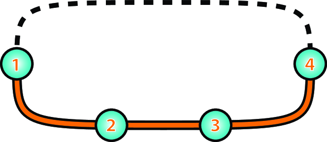
Figure 1: Sample network with three short-range connections and one long-range connection (dashed line). If we want to reach the node 4 departing from 1, we can choose two shortest paths: $\{1,2,3,4\}$, which uses only short-range connections and $\{1,4\}$, which uses the long-range connection. In the point of view of the time spended to travel, there is no difference between the two paths if displacement velocities are the same along the two types of edges. In the other hand, if we can move faster in the long-range connection, we should choose the second path.

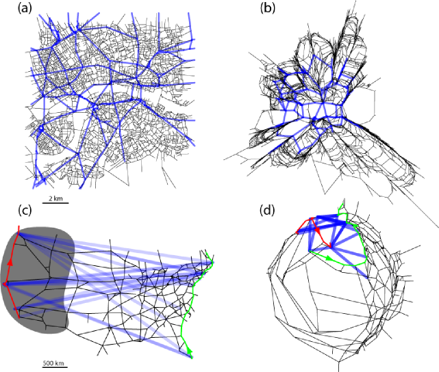
Figure 2: (a) The network of London streets and respective underground system (the latter in blue). (b) Layout obtained by multidimensional scaling. (c) Network of US Interstate Highway system enhanced by twenty of the most important links US Airlines links (in blue). (d) Layout obtained by multidimensional scaling. The adoped values of $\alpha$ were $\alpha=3$ for LSN and $\alpha=6$ for USHN. The red and green lines were placed in (c) and (d) just to identify the final positions on the west and east coast. Observe that the length of an edge in (b) and (d) is proportional to the time required to cross that edge.

In order to illustrate the importance of the space on the transport properties, we show in Figure 1 a simple embeded network with three short-range connection and one long-range connection. If we want to reach node 4 after departing from 1, we can choose two different shortest paths (ie. paths with the minimum total length): $\{1,2,3,4\}$ or $\{1,4\}$. Observe that the first path only uses short-range connections, while the second option uses a long-range link. It is clear that if the displacement velocity is fixed for both types of connections, there is no advantage to use the first or second option. However, as we will see, a substantially different result can be obtained when we consider different displacement velocities for long and short-range connections.

Commonly, real transportation networks are generalizations of the simple situations discussed above. Real networks are embeded in three-dimensional spaces and display regular properties, in which each node is connected to a few number of neighboors through short-range connections. This strategy reduces the building cost of real-world structures, which have their costs proportional to the total length of the system Barthélemy and Flammini (2008). In addition, the network is enhanced by a few number of long-range links that spans the space. The key point here is to consider that the displacement velocity through the short-range and long-range connections are different. While the displacement along the short-range connections occurs at velocity $v_{s}$, in long range-connection this velocity is $v_{l}=\alpha v_{s}$, with $\alpha>1$.

In the current paper we study two important real-world systems characterized by the features discribed above, ie. they have two types of connections with respectively different displacement velocities. The systems that will be considered are (a) the network of streets of London plus the respective underground system and (b) the US highway plus some of the main US airlines connections. We will use the multidimensional scaling in order to visualize the effect of the long-range and will then quantify the importance of these connections on the transportation properties as well.

This paper is organized as follow: we start by presenting and discussing the networks used here. Next, the multidimensional scaling is used to visualize the effects of the network topology. We then use an attack dynamics in order to quantify the importance of the long-range connections as compared to the short-range ones. Finally, we present the main conclusions and prospects for further investigation.

II Description of the data

In this section we will how both networks used in this paper were constructed: (a) the network of streets of London plus the respective underground system and (b) the US highway plus some of the main US airlines connections.

II.1 London Streets Network (LSN)

The central region of London, corresponding to about 13km$\times$13km, was mapped into a network where each node corresponds to the confluence of two or more streets. Also, the underground system of London respective to the same region was then appended into this network. Each underground station was replaced by its closer node from the respective street network. For this network (henceforth called LSN), we have $\alpha\approx 3$ and $3\%$ of the total number of edges correspond to long-range connections. The final network contains 5963 nodes and it has an average degree of 2.81. Figure 2(a) shows the final version of this network, where the long-range-connections are depicted in blue. Observe that, for this network, the long-range connections are 5 times larger than short-range connections, in the average.

II.2 US Highways Network (USHN)

The sencond network (USHN) considered in this paper was built using the American highway system enhanced by twenty of the most important airlines connections. The importance of the airline connections was quantified according the number of passengers that they transport. In this network, the confluences of two or more highways were mapped into nodes. Two nodes are linked if a highway connects them. Moreover, the extremities of the airline connections were replaced by the closest nodes from the highway system. For this network, we have $\alpha\approx 6$ and the fraction of edges corresponding to long-range-connections is $3\%$, again. The final version of this network is showed in Figure 2(b) and it contains 428 nodes with an average degree of 3.15. It is interesting to observe that almost all long-range connection tend to link the the west coast to the east coast. In average, we observed in this network, long-range connections 40 times larger than short-range connections.

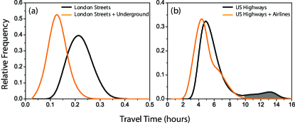
Figure 3: Effect of the long-range connection in the distribution of the traveling time for the (a) LSN and (b) USHN. In both cases, the distributions were shifted to left when the long-range connection were considered (orange lines). As we expected, this result indicates that the time required to travel between two nodes decreases in the presence of the long-range connections. In (a) the average value decreases 42% while in (b) it decreases 20%. Observe that these results are affected by the number of long-range connections considered in each system. The average travel time reduction per long-range connection is about 0.14% in (a) and 2% in (b).

III Visualizing the effect of the long-range connections

We applied the classical mutidimensional scaling  Kruskal (1964); Berthold and Hand (2003) on the networks in order to visualize the effect of the long-range connections. This technique provides a powerfull way for obtaining the nodes positions from a dissimilarity matrix. We denote by $\tau_{i,j}$ the dissimilarity between the nodes $i$ and $j$. In our case, this dissimilarity corresponds to the minimum traveling time to reach the destination node $j$ after departing from $i$. In order to evaluate the value of $\tau_{i,j}$ each edge $(i,j)$ of the network received an weight corresponding to $\tau_{i,j}=\ell_{i,j}/v_{i,j}$, where $\ell_{i,j}$ is the Euclidean distance between $i$ and $j$ and $v_{i,j}=v_{s}$ if $(i,j)$ is a short-range connection or $v_{i,j}=\alpha v_{s}$ if $(i,j)$ is a long-range connection. The dissimilarity matrix is defined as the $N\times N$ symmetric matrix $\mathbf{T}$, which has elements $\tau_{i,j}$. Now, the following matrix is obtained from $\mathbf{T}$:

$$\mathbf{B}=-\frac{1}{2}\left(\mathbf{I}-\frac{1}{N}\mathbf{U}\mathbf{U}^{T}\right)\mathbf{T}^{\prime}\left(\mathbf{I}-\frac{1}{N}\mathbf{U}\mathbf{U}^{T}\right),$$ (1)

where $\mathbf{U}$ is a vector $N\times 1$ whose elements are all equal to one, $\mathbf{I}$ is the $N\times N$ identity matrix and $\mathbf{T}^{\prime}$ is a matrix whose elements are equal to the square of the elements of $\mathbf{T}$, ie. $\tau^{\prime}_{i,j}=\tau^{2}_{i,j}$. The eigenvalues of $\mathbf{B}$ are then identified, and only those which are larger than zero are considered in order to build the next matrix, $\mathbf{E}$. Then, these $n\leq N$ eigenvalues are sorted in decreasing order, yielding the sequence $\lambda_{1}>\lambda_{2}>\ldots>\lambda_{n}>0$. The respective eigenvectors are stacked as columns of a matrix $\mathbf{E}$ with dimension $N\times n$. The coordinates of the $N$ nodes can now be obtained, up to a rigid body transformation, as:

$$\mathbf{X}=\mathbf{E}\left(\begin{array}[]{cccc}\sqrt{\lambda_{1}}&0&\ldots&0\\ 0&\sqrt{\lambda_{2}}&\ldots&0\\ \ldots&\ldots&\ldots&\ldots\\ 0&0&\ldots&\sqrt{\lambda_{n}}\\ \end{array}\right).$$ (2)

The dimension of the final coordinates is approximately given by the number of non-null eigenvalues, $n$. The higher the number of constrainments of the dissimilarity matrix, the larger is the number of dimensions required. Here we considered only two first eigenvectors to visualize the final aspect of the transportation networks. The results are showed in Figure 2(b) and Figure 2(d) for LSN and USHN, respectvelly.

It is clear from the Figure 2(b) that the peripheral regions of London were brought close to the central region. For the USHN case - Figure 2(d), one can observe a folding effect bringing together the west and the east coast over the US map. In both these figures, the edge lengths are proportional to the traveling time required to cross that respective edge. Thus, we expected that the travel time averaged over all nodes of each network (average travel time) has decreased as a consequence of the addition of long-range connections. This was confirmed by the results shown in Figure 3, where we consider the distribution of the travel time for both networks with and without the long-range connections. It is possible to observe that in both cases the traveling time was significantly decreased. Moreover, in the case of the USHN, we can also note that the inclusion of the long-range connections had a strong effect on the secondary peak of the time travel distribution (gray region of Figure 3(b)), meaning that the access to several nodes was improved. We verifyed that these nodes, which had they access improved, belong to the west coast and they are identified by the gray region in Figure 2(c).

IV Quantifying the importance of the long-range connections

In order to investigate how the long-range connections can contribute to improve the flow in transport networks, we performed a deletion process under the USHN. At each time step, we chose a random edge of the considered network and then checked if its respectively deletion kept the network connected. If that was true, we deleted this edge and re-evaluated the average traveling time. Next, a new edge was chosen, and so on. This process finishes when no edges can be deleted. The following configurations were considered: (i) deletion of the short-range connections from the highways network without long-range connections; (ii) deletion of the short-range connections from the highways network with long-range connections; (iii) deletion of the long-range connections from the highways network with long-range connections; and (iv) deletion of the short-range and long-range connections from the highways network with long-range connections. The results are shown in Figure 3. As one can see, the configurations (i), (ii) and (iv) have similar results and they converge to a linear function with slope $\gamma=1.6$ when more than 30 edges are deleted. This behavior was not observed in the case (iii), which diverged quickly while the percentual increase of the average travel time reached about $25\%$ when twenty long-range connections were deleted. For the other cases, it increased only $2.5\%$ in the average. In addition, we can observe in Figure 4 that about a hundred deleted edges are required in order to cause the same damage in (i), (ii) and (iv) as in (iii). These results show that the long-range connection are able to substantially improve the resilience in networks, but at the same time, they can be considered as potential targets for preferential attacks.

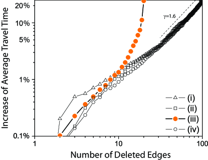
Figure 4: Behavior of the average travel time during the edges deletion process. The edges were deleted using four different strategies. In the first case, we considered the (i) US highways network without long-range connections and deleted its edges one by one (triangles). Next we considered the US highways network with long-range connections and deleted the (ii) short-range connections (squares), (iii) long-range connections (filled circles) and (iv) random connections (open circles). After each deletion, the new average travel time was re-evaluated. Also, along the deletion process, we chose edges that kept the network connected. The y-axis correspond to the percentual increase of the average travel time.

V Conclusions

All in all, the results showed here lead us to believe that the reduction effect of the travel time observed above can be considered as an analogue of the small-world effect for the transportation networks. For these networks, the nodes have a very-well defined positions on space and tend to be linked with the neighboors trought short-range connections in order to minimize the building cost. If a few number of long-range connections are introduced in the network, overcomming the original regular structure, the time spended to travel in this network decreases significantly. It is important to note that this result becomes valid when the displacement velocities along the short-range ($v_{s}$) and long-range ($v_{l}$) connections are different.

We studied two real transport networks: (i) the London streets networks plus the respective underground system (LNS) and (ii) the US highway system enhanced by some of the main airline connections (USHN). For these systems, we considered $v_{l}=\alpha v_{s}$, with $\alpha=3$ for LSN and $\alpha=6$ for USHN. By using the multidimensional scaling methodology, we showed how the long-range connections change the effective geography of the networks, bringing together regions that are far away in the maps. These visual results provided by the multidimensional scaling were confirmed by the left-shift observed in the time traveling distributions, meaning that the the addition of the long range-connections descreased the time spent while traveling in the networks.

The importance of the long-range connections againts the short-range ones was quantifyed b yusing an edge deletion process, in which, at each time step, an edge of the networks was deleted and the time travel was re-evaluated. We observed that when the deletion is performed only over the long-range connections, the time travel diverges quickly, while it has a linear behavior when the other deletion strategies are considered.