Some planar isospectral domains

Abstract

We give a number of examples of isospectral pairs of plane domains, and a particularly simple method of proving isospectrality. One of our examples is a pair of domains that are not only isospectral but homophonic: Each domain has a distinguished point such that corresponding normalized Dirichlet eigenfunctions take equal values at the distinguished points. This shows that one really can’t hear the shape of a drum.

1 Introduction

In 1965, Mark Kac [6] asked, ‘Can one hear the shape of a drum?’, so popularizing the question of whether there can exist two non-congruent isospectral domains in the plane. In the ensuing 25 years many examples of isospectral manifolds were found, whose dimensions, topology, and curvature properties gradually approached those of the plane. Recently, Gordon, Webb, and Wolpert [5] finally reduced the examples into the plane. In this note, we give a number of examples, and a particularly simple method of proof. One of our examples (see Figure 1) is a pair of domains that are not only isospectral but homophonic: Each domain has a distinguished point such that corresponding normalized Dirichlet eigenfunctions take equal values at the distinguished points. We interpret this to mean that if the corresponding ‘drums’ are struck at these special points, then they ‘sound the same’ in the very strong sense that every frequency will be excited to the same intensity for each. This shows that one really can’t hear the shape of a drum.

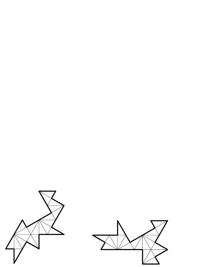
Figure 1: Homophonic domains. These drums sound the same when struck at the interior points where six triangles meet.

2 Transplantation

The following transplantation proof was first applied to Riemann surfaces by Buser [1]. For our domains this proof turns out to be particularly easy.

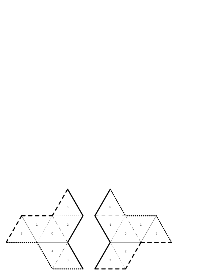
Figure 2: Propeller example.

Consider the two propeller-shaped regions shown in Figure 2. Each region consists of seven equilateral triangles (labelled in some unspecified way). Our first pair of examples is obtained from these by replacing the equilateral triangles by acute-angled scalene triangles, all congruent to each other. The propellers are triangulated by these triangles in such a way that any two triangles that meet along a line are mirror images in that line, as in Figure 3. In both propellers the central triangle has a distinguishing property: its sides connect the three inward corners of the propeller. The position of the propellers in Figure 3 is such that the unique isometry from the central triangle on the left-hand side to the central triangle on the right-hand side is a translation. This translation does not map the propellers onto one another and so they are not isometric.

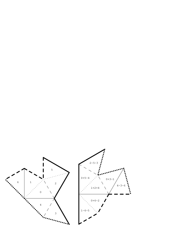
Figure 3: Warped propeller.

Now let $\lambda$ be any real number, and $f$ any eigenfunction of the Laplacian with eigenvalue $\lambda$ for the Dirichlet problem corresponding to the left-hand propeller. Let $f_{0},f_{1},\ldots,f_{6}$ denote the functions obtained by restricting $f$ to each of the 7 triangles of the left-hand propeller, as indicated on the left in Figure 3. For brevity, we write $\bf 0$ for $f_{0}$, $\bf 1$ for $f_{1}$, etc. The Dirichlet boundary condition is that $f$ must vanish on each boundary-segment. Using the reflection principle, this is equivalent to the assertion that $f$ would go into $-f$ if continued as a smooth eigenfunction across any boundary-segment. (More precisely it goes into $-f\circ\sigma$ where $\sigma$ is the reflection on the boundary segment.)

On the right in Figure 3, we show how to obtain from $f$ another eigenfunction of eigenvalue $\lambda$, this time for the right-hand propeller. In the central triangle, we put the function $\bf 1+\bf 2+\bf 4$. By this we mean the function $f_{1}\circ\tau_{1}+f_{2}\circ\tau_{2}+f_{4}\circ\tau_{4}$ where for $k=1,2,4$, $\tau_{k}$ is the isometry from the central triangle of the right-hand propeller to the triangle labelled $k$ on the left-hand propeller. Now we see from the left-hand side that the functions $\bf 1,\bf 2,\bf 4$ continue smoothly across dotted lines into copies of the functions $\bf 0,\bf 5,-\bf 4$ respectively, so that their sum continues into $\bf 0+\bf 5-\bf 4$ as shown. The reader should check in a similar way that this continues across a solid line to $\bf 4-\bf 5-\bf 0$ (its negative), and across a dashed line to $\bf 2-\bf 5-\bf 3$, which continues across either a solid or dotted line to its own negative. These assertions, together with the similar ones obtained by symmetry (i.e. cyclic permutation of the arms of the propellers), are enough to show that the transplanted function is an eigenfunction of eigenvalue $\lambda$ that vanishes along each boundary segment of the right-hand propeller.

So we have defined a linear map which for each $\lambda$ takes the $\lambda$-eigenspace for the left-hand propeller to the $\lambda$-eigenspace for the right-hand one. This is easily checked to be a non-singular map, and so the dimension of the eigenspace on the right-hand side is larger or equal the dimension on the left-hand side. Since the same transplantation may also be applied in the reversed direction the dimensions are equal. This holds for each $\lambda$, and so the two propellers are Dirichlet isospectral.

In fact they are also Neumann isospectral, as can be seen by a similar transplantation proof obtained by replacing every minus sign in the above by a plus sign. (Going from Neumann to Dirichlet is almost as easy: Just color the triangles on each side alternately black and white, and attach minus signs on the right to function elements that have moved from black to white or vice versa.)

In the propeller example, each of the seven function elements on the left got transplanted into three triangles on the right, and we verified that it all fits together seamlessly. If we hadn’t been given the transplantation rule, we could have worked it out as follows: We start by transplanting the function element $\bf 1$ into the central triangle on the right; on the left $\bf 1$ continues across a dotted line to $\bf 0$, so we stick $\bf 0$ in the triangle across the dotted line on the right; on the left $\bf 0$ continues across the solid line to $\bf 4$, and since on the right the solid side of the triangle containing $\bf 0$ is a boundary edge, we stick a $\bf 4$ in along with the $\bf 0$ (don’t worry about signs—we can fill them in afterwards using the black and white coloring of the triangles); now since on the left $\bf 4$ continues across a dotted line to itself we stick a $\bf 4$ into the center along with the $\bf 1$ we started with; and so on until we have three function elements in each triangle on the right and the whole thing fits together seamlessly.

If we had begun by putting $\bf 0$ into the central triangle on the right, rather than $\bf 1$, then we would have ended up with four function elements in each triangle, namely, the complement in the set $\{\bf 0,\bf 1,\ldots,\bf 6\}$ of the original three; This gives a second transplantation mapping. Call the original mapping $T_{3}$, and the complementary mapping $T_{4}$. Any linear combination $aT_{3}+bT_{4},\;a\neq b$ will also be a transplantation mapping, and if we take for $(a,b)$ one of the four solutions to the equations $3a^{2}+4b^{2}=1$, $a^{2}+4ab+2b^{2}=0$, our transplantation mapping becomes norm-preserving.

Now consider the pair of putatively homophonic domains shown in Figure 1 above. In this case we find two complementary transplantation mappings $T_{5}$ and $T_{16}$. The linear combination $aT_{5}+bT_{16}$ is a norm-preserving mapping if $5a^{2}+16b^{2}=1$ and $a^{2}+8ab+12b^{2}=0$, that is, if $(a,b)=\pm(1/3,-1/6)$ or $(a,b)=\pm(3/7,-1/{14})$. In the Dirichlet case, transplantation is kind to the values of the transplanted functions at the special interior points where six triangles meet. With the proper choice of sign, the Dirichlet incarnation of $T_{5}$ multiplies the special value by 2, the Dirichlet incarnation of $T_{16}$ multiplies the special value by $-2$, and the four norm-preserving linear combinations $aT_{5}+bT_{16}$ specified above multiply it by $2(a-b)=\pm 1$. Thus we can convert an orthonormal basis of Dirichlet eigenfunctions on the left to one on the right so that corresponding functions take on the same special value. This shows that the two domains are homophonic, or more specifically, Dirichlet homophonic. There is no similar reason for these domains to be Neumann homophonic, and, in fact, we do not know of any pair of non-congruent Neumann homophonic domains.

3 Gallery of examples

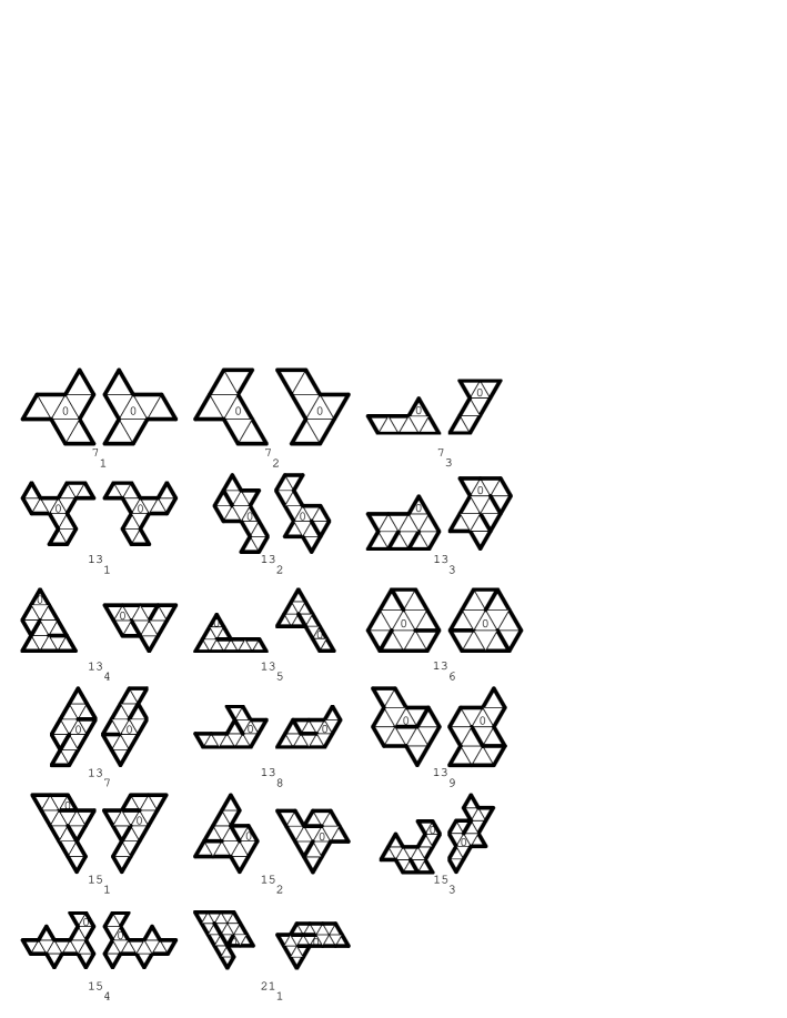
Figure 4: Isospectral domains.

Figure 4 shows pairs of diagrams representing domains whose isospectrality can be verified using the method of transplantation. Each pair of diagrams represents not a single pair of isospectral domains, but a whole family of pairs of isospectral domains, gotten by replacing the equilateral triangles with general triangles so that the triangles labelled 0 are mapped onto one another by a translation and the remaining triangles are obtained from these by the appropriate sequence of reflections. We have seen two examples of this already, in Figures 3 and 1. Further examples generated in this way are shown in Section 5.

The pair $7_{1}$ is the pair of propeller diagrams discussed in detail above. The pair $7_{3}$ yields a simplified version of the pair of isospectral domains given by Gordon, Webb, and Wolpert [5], [4], which was obtained by bisecting a pair of flat but non-planar isospectral domains given earlier by Buser [2]. The pair $21_{1}$ yields the homophonic domains shown in Figure 1 above. In this case we must be careful to choose the relevant angle of our generating triangle to be $2\pi/6$ since six of these angles meet around a vertex in each domain. If we do not choose the angle to be $2\pi/6$, then instead of planar domains we get a pair of isospectral cone-manifolds.

Note that in order for the pair $13_{6}$ to yield a pair of non-overlapping non-congruent domains we must decrease all three angles simultaneously, which we can do by using hyperbolic triangles in place of Euclidean triangles. Using hyperbolic triangles, we can easily produce isospectral pairs of convex domains in the hyperbolic plane, but we do not know of any such pairs in the Euclidean plane.

4 More about the examples

The examples in the previous section were obtained by applying a theorem of Sunada [7]. Let $G$ be a finite group. Call two subgroups $A$ and $B$ of $G$ isospectral if each element of $G$ belongs to just as many conjugates of $A$ as of $B$. (This is equivalent to requiring that $A$ and $B$ have the same number of elements in each conjugacy class of $G$.) Sunada’s theorem states that if $G$ acts on a manifold $M$ and $A$ and $B$ are isospectral subgroups of $G$, then the quotient spaces of $M$ by $A$ and $B$ are isospectral.

The tables in this section show for each of the examples a trio of elements which generate the appropriate $G$, in two distinct permutation representations. The isospectral subgroups $A$ and $B$ are the point-stabilizers in these two permutation representations.

For the example $7_{1}$, the details are as follows. $G_{0}$ is the group of motions of the hyperbolic plane generated by the reflections $a_{0},b_{0},c_{0}$ in the sides of a triangle whose three angles are $\pi/4$. In Conway’s orbifold notation (see [3]), $G_{0}=*444$. $G_{0}$ has a homomorphism $a_{0}\mapsto a,b_{0}\mapsto b,c_{0}\mapsto c$ onto the finite group $G=L_{3}(2)$ (also known as $PSL(3,2)$), the automorphism group of the projective plane of order 2. The generators of $G$ act on the points and lines of this plane (with respect to some unspecified numbering of the points and lines) as follows:

$$a = (0\ 1)(2\ 5)\ /\ (0\ 4)(2\ 3)$$

$$b = (0\ 2)(4\ 3)\ /\ (0\ 1)(4\ 6)$$

$$c = (0\ 4)(1\ 6)\ /\ (0\ 2)(1\ 5),$$

where the actions on points and lines are separated by $/$.

The group $G$ has two subgroups $A$ and $B$ of index 7, namely the stabilizers of a point or a line. The preimages $A_{0}$ and $B_{0}$ of these two groups in $G_{0}$ have fundamental regions that consist of 7 copies of the original triangle, glued together as in Figure 2. Each of these is a hexagon of angles $\pi/4,\pi/2,\pi/4,\pi/2,\pi/4,\pi/2$, and so each of $A_{0}$ and $B_{0}$ is a copy of the reflection group $*424242$.

The preimage in $G_{0}$ of the trivial subgroup of $G$ is a group $K_{0}$ of index 168. The quotient of the hyperbolic plane by $K_{0}$ is a 23-fold cross-surface (that is to say, the connected sum of 23 real projective planes), so that in Conway’s orbifold notation $K_{0}=\times^{23}$. Deforming the metric on this 23-fold cross surface by replacing its hyperbolic triangles by scalene Euclidean triangles yields a cone-manifold $M$ whose quotients by $A$ and $B$ are non-congruent planar isospectral domains.

Tables 1 and 2 display the corresponding information for our other examples.

$$\begin{array}[]{lllllcl}\mbox{Pair}&\mbox{Generators}&K_{0}&G_{0}&A_{0},B_{0}&G&\mbox{Notes}\\ \\ 7_{1}&a,b,c&\times^{23}&*444&*424242&L_{3}(2)\\ 7_{2}&a,b^{\prime},c&\times^{16}&*443&*42423&\prime\prime&a^{\prime}=cac\\ 7_{3}&a^{\prime},b^{\prime},c&\times^{9}&*433&*4233&\prime\prime&b^{\prime}=aba\\ 13_{1}&d,e,f&\times^{704}&*444&*422422422&L_{3}(3)\\ 13_{2}&d,e^{\prime},f&\times^{938}&*644&*6622342242&\prime\prime&e^{\prime}=ded\\ 13_{3}&d^{\prime},e^{\prime},f&\times^{1172}&*664&*62234263662&\prime\prime&d^{\prime}=fdf\\ 13_{4}&d^{\prime},e^{\prime},f^{\prime}&\times^{938}&*663&*633626362&\prime\prime&f^{\prime}=e^{\prime}fe^{\prime}\\ 13_{5}&d^{\prime},e^{\prime\prime},f^{\prime}&\times^{470}&*633&*663332&\prime\prime&e^{\prime\prime}=d^{\prime}e^{\prime}d^{\prime}\\ 13_{6}&g,h,i&\times^{1406}&*666&*632663266326&\prime\prime\\ 13_{7}&g,h^{\prime},i&\times^{938}&*663&*632666233&\prime\prime&h^{\prime}=ghg\\ 13_{8}&g^{\prime},h^{\prime},i&\times^{704}&*643&*63436222,*62633224&\prime\prime&g^{\prime}=igi\\ 13_{9}&g^{\prime},h^{\prime},i^{\prime}&\times^{938}&*644&*6262242243&\prime\prime&i^{\prime}=g^{\prime}ig^{\prime}\\ 15_{1}&j,k,l&\times^{3362}&*663&*63362333222&L_{4}(2)\\ 15_{2}&j,k,l^{\prime}&\times^{4202}&*664&*6262234342242&\prime\prime&l^{\prime}=jlj\\ 15_{3}&j^{\prime},k,l^{\prime}&\times^{3362}&*644&*62234424242,*62422243442&\prime\prime&j^{\prime}=kjk\\ 15_{4}&j^{\prime},k^{\prime},l^{\prime}&\times^{2522}&*444&*444222442&\prime\prime&k^{\prime}=l^{\prime}kl^{\prime}\\ 21_{1}&p,q,r&\times^{1682}&*633&*63633332,*66333323&L_{3}(4)\\ \end{array}$$

Table 1: Specifications.

$$\begin{array}[]{lll}a&=&(0\ 1)(2\ 5)\ /\ (0\ 4)(2\ 3)\\ b&=&(0\ 2)(4\ 3)\ /\ (0\ 1)(4\ 6)\\ c&=&(0\ 4)(1\ 6)\ /\ (0\ 2)(1\ 5)\\ \\ d&=&(0\ 12)(1\ 10)(3\ 5)(6\ 7)\ /\ (0\ 4)(2\ 3)(6\ 8)(9\ 10)\\ e&=&(0\ 10)(3\ 4)(9\ 2)(5\ 8)\ /\ (0\ 12)(6\ 9)(5\ 11)(1\ 4)\\ f&=&(0\ 4)(9\ 12)(1\ 6)(2\ 11)\ /\ (0\ 10)(5\ 1)(2\ 7)(3\ 12)\\ \\ g&=&(0\ 2)(1\ 7)(3\ 6)(5\ 10)\ /\ (0\ 7)(3\ 11)(6\ 8)(9\ 12)\\ h&=&(0\ 6)(3\ 8)(9\ 5)(2\ 4)\ /\ (0\ 8)(9\ 7)(5\ 11)(1\ 10)\\ i&=&(0\ 5)(9\ 11)(1\ 2)(6\ 12)\ /\ (0\ 11)(1\ 8)(2\ 7)(3\ 4)\\ \\ j&=&(0\ 14)(4\ 5)(9\ 10)(1\ 12)(7\ 11)(2\ 6)\\ &/&(0\ 11)(1\ 5)(3\ 4)(6\ 10)(8\ 9)(13\ 14)\\ k&=&(4\ 6)(1\ 13)(8\ 9)(2\ 7)\\ &/&(0\ 10)(1\ 2)(6\ 9)(12\ 14)\\ l&=&(14\ 1)(3\ 4)(12\ 2)(8\ 11)\\ &/&(0\ 5)(2\ 4)(6\ 7)(11\ 14)\\ \\ p&=&(2\ 7)(3\ 11)(5\ 12)(8\ 18)(13\ 14)(15\ 17)(16\ 20)\\ &/&(0\ 1)(4\ 17)(7\ 12)(9\ 16)(10\ 20)(11\ 13)(15\ 19)\\ q&=&(0\ 17)(3\ 8)(4\ 12)(6\ 13)(9\ 19)(14\ 15)(16\ 18)\\ &/&(0\ 20)(3\ 16)(6\ 11)(8\ 15)(9\ 19)(10\ 12)(14\ 18)\\ r&=&(1\ 8)(2\ 16)(4\ 11)(5\ 19)(7\ 14)(10\ 17)(13\ 20)\\ &/&(1\ 8)(2\ 16)(4\ 11)(5\ 19)(7\ 14)(10\ 17)(13\ 20)\par\end{array}$$

Table 2: Permutations.

Note that the permutations in Table 2 correspond to the neighboring relations in Figure 4. In the propeller example, for instance, the pairs 0, 1 and 2, 5 are neighbors along a dotted line on the left-hand side, and 0, 4 and 2, 3 are neighbors along a dotted line on the right-hand side. Accordingly, we have the permutations a = (0 1)(2 5)  / (0 4)(2 3), etc. Similar relations will hold in the other pairs of diagrams if the triangles are properly labelled.

5 Special cases of isospectral pairs

Figure 5 shows some interesting special cases of isospectral pairs.

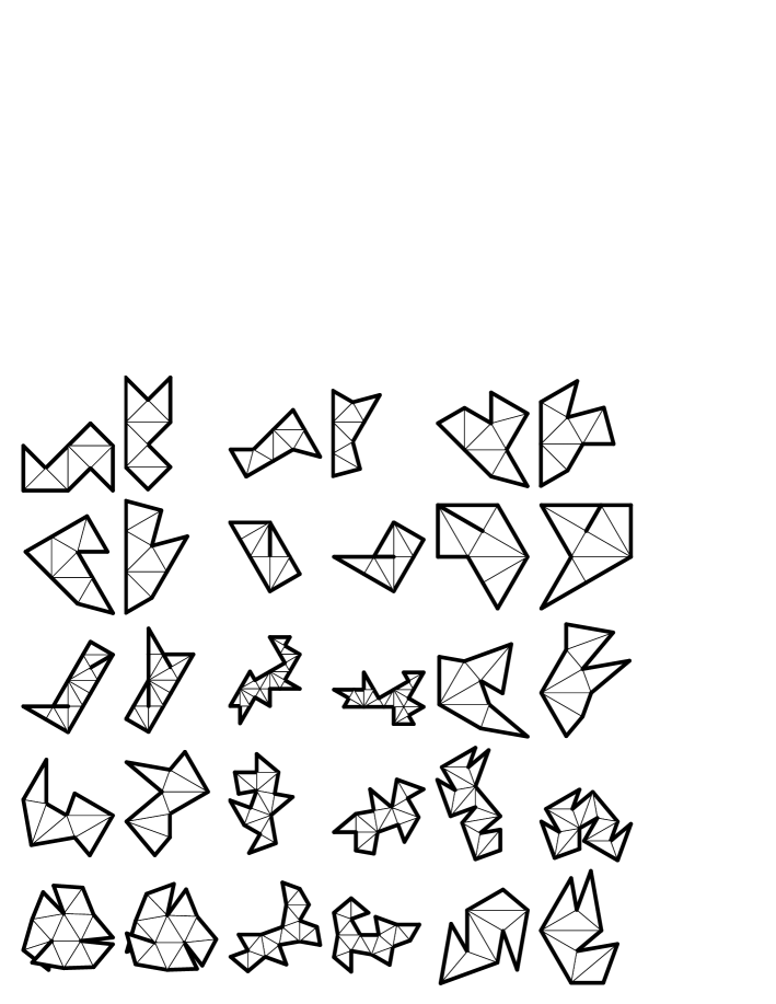
Figure 5: Special cases.

References

- [1] P. Buser. Isospectral Riemann surfaces. Ann. Inst. Fourier (Grenoble), 36:167–192, 1986.
- [2] P. Buser. Cayley graphs and planar isospectral domains. In T. Sunada, editor, Geometry and Analysis on Manifolds (Lecture Notes in Math. 1339), pages 64–77. Springer, 1988.
- [3] J. H. Conway. The orbifold notation for surface groups. In M. W. Liebeck and J. Saxl, editors, Groups, Combinatorics and Geometry, pages 438–447. Cambridge Univ. Press, Cambridge, 1992.
- [4] C. Gordon, D. Webb, and S. Wolpert. Isospectral plane domains and surfaces via Riemannian orbifolds. Invent. Math., 110:1–22, 1992.
- [5] C. Gordon, D. Webb, and S. Wolpert. One cannot hear the shape of a drum. Bull. Amer. Math. Soc., 27:134–138, 1992.
- [6] M. Kac. Can one hear the shape of a drum? Amer. Math. Monthly, 73, 1966.
- [7] T. Sunada. Riemannian coverings and isospectral manifolds. Ann. of Math., 121:169–186, 1985.