Quantum Diffusion and Delocalization for Band Matrices with General Distribution

Abstract

We consider Hermitian and symmetric random band matrices $H$ in $d\geqslant 1$ dimensions. The matrix elements $H_{xy}$, indexed by $x,y\in\Lambda\subset\mathbb{Z}^{d}$, are independent and their variances satisfy $\sigma_{xy}^{2}:=\mathbb{E}\lvert H_{xy}\rvert^{2}=W^{-d}f((x-y)/W)$ for some probability density $f$. We assume that the law of each matrix element $H_{xy}$ is symmetric and exhibits subexponential decay. We prove that the time evolution of a quantum particle subject to the Hamiltonian $H$ is diffusive on time scales $t\ll W^{d/3}$. We also show that the localization length of the eigenvectors of $H$ is larger than a factor $W^{d/6}$ times the band width $W$. All results are uniform in the size $\lvert\Lambda\rvert$ of the matrix. This extends our recent result [1] to general band matrices. As another consequence of our proof we show that, for a larger class of random matrices satisfying $\sum_{x}\sigma_{xy}^{2}=1$ for all $y$, the largest eigenvalue of $H$ is bounded with high probability by $2+M^{-2/3+\varepsilon}$ for any $\varepsilon>0$, where $M\mathrel{\mathop{:}}=1/(\max_{x,y}\sigma_{xy}^{2})$.

AMS Subject Classification: 15B52, 82B44, 82C44

Keywords: Random band matrix, renormalization, localization length.

1 Introduction

We proved recently [1] that the quantum time evolution $\mathrm{e}^{-\mathrm{i}tH/2}$ generated by a band matrix $H$ with band width $W$ is diffusive on time scales $t\ll W^{d/3}$, where $d=1,2,3,\ldots$ is the number of spatial dimensions. As a consequence, we showed that typical eigenvectors are delocalized on a scale at least $W^{1+d/6}$, i.e. the localization length is much larger than the band width. A key assumption in [1] was that the matrix entries $H_{xy}$ satisfy

$$\lvert H_{xy}\rvert^{2}\;=\;\frac{1}{M}\bm{\mathrm{1}}(1\leqslant\lvert x-y\rvert\leqslant W)\,,\qquad x,y\in\Lambda,$$ (1.1)

where $\Lambda$ is a large finite box in $\mathbb{Z}^{d}$ and $M\sim W^{d}$ is a normalization to ensure that $\sum_{y}|H_{xy}|^{2}=1$. For the physical significance of this result in connection with the extended states conjecture for random Schrödinger operators, see the introduction of [1], where we also presented an overview of related results and references.

The goal of this paper is to replace the rather restrictive deterministic condition (1.1) on the matrix elements with a natural general class of random variables. We consider symmetric or Hermitian random band matrices $H=(H_{xy})$ such that $\mathbb{E}H_{xy}=0$ and the variances $\sigma_{xy}^{2}\mathrel{\mathop{:}}=\mathbb{E}\lvert H_{xy}^{2}\rvert$ are given by $\sigma_{xy}^{2}=W^{-d}f\bigl{(}{(x-y)/W}\bigr{)}$, where $f$ is a nonnegative function satisfying $\int_{\mathbb{R}^{d}}\mathrm{d}x\,f(x)=1$. Thus, $f$ describes the shape of a band of width $W$. The matrix entries are assumed to have an even law with subexponential decay. Under these assumptions we show that all results of [1] remain valid.

The proof of quantum diffusion for general band matrices is considerably more involved than for matrices satisfying (1.1). Our proofs are based on an expansion in so-called nonbacktracking powers of $H$. As observed by Feldheim and Sodin [2, 5], under the assumption (1.1) these powers satisfy a simple algebraic recursion relation which immediately implies that they are given by Chebyshev polynomials in $H$. In the language of perturbative quantum field theory, the nonbacktracking powers correspond to a self-energy renormalization up to all orders. The underlying algebraic identity, however, heavily relies on the special form (1.1). If (1.1) does not hold, the renormalization is no longer algebraically exact and the recursion relation becomes much more complicated. There are two main reasons for this complication. The first is that the absolute value of each matrix element is genuinely random, and hence powers of matrix elements $|H_{xy}|^{k}$ cannot be replaced by a constant. The second reason is that the variance $\sigma_{xy}^{2}$ is no longer given by a step function in $x-y$. These two complications give rise to different types of error terms that substantially increase the complexity of the Feynman graphs to be estimated. For instance if, instead of (1.1), we assumed

$$\sigma_{xy}^{2}=\mathbb{E}\lvert H_{xy}\rvert^{2}\;=\;\frac{1}{M}\bm{\mathrm{1}}(1\leqslant\lvert x-y\rvert\leqslant W)\,,\qquad x,y,\in\Lambda,$$ (1.2)

i.e. if the band were given by a step function, then our proof would be simpler (in the language of the graphical representation of Section 6, we would not have any wiggly lines).

We remark that some of the additional complications when considering ensembles more general than (1.1) have been tackled in [2] and [5]. In particular, Feldheim and Sodin, in Section III of [2], describe how to extend their result on the expectation value of traces of Chebyshev polynomials of Wigner matrices from (1.1) to more general distributions. In Section 9 of his paper on band matrices [5], Sodin states that the procedure of Section III of [2] can be extended to band matrices satisfying the restriction (1.2), but no details are given. It seems, however, that $\sigma_{xy}^{2}$ being either a fixed constant or zero plays an important role. In this paper we consider more general band matrices (assuming less decay of the law of the matrix elements, and an arbitrary band shape), and we need to compute squares of matrix elements. Hence the structure of our expansion is more involved, and a novel approach is required to control it.

As a simple consequence of our proof, we also derive a bound on the largest eigenvalue $\lambda_{\mathrm{max}}$ of a band matrix. This result holds in fact for a more general class of random matrices in which the spatial structure (and hence the dependence on the spatial dimension $d$) is absent. The relevant parameter for such matrices is

$$M\;\mathrel{\mathop{:}}=\;\frac{1}{\max_{x,y}\mathbb{E}\lvert H_{xy}^{2}\rvert}\,,$$

characterizing, very roughly, the number of nontrivial entries in each row of $H$. It is easy to see that, in the special case of $d$-dimensional band matrices introduced in Section 2, we have $M\sim CW^{d}$ where $W$ is the band width; for a Wigner matrix we have $M=N$, where $N$ denotes the size of the matrix. We show that $\lambda_{\mathrm{max}}\leqslant 2+M^{-2/3+\varepsilon}$ with high probability for any $\varepsilon>0$, provided that $\log N\ll M^{c\varepsilon}$; here $c$ is a constant. For a smaller class of band matrices, Sodin [5] previously proved that $\lambda_{\mathrm{max}}=2+o(1)$ in distribution, under the assumption $\log N\ll M$. (In fact, for $M\ll N^{5/6}$ he computes the asymptotic integrated density of states near the spectral edge, and for $M\gg N^{5/6}$ he even identifies the limiting distribution of the largest eigenvalue as the Tracy-Widom distribution.) For other previous results on the largest eigenvalue of random band matrices see the references in [5]. In the special case ($M=N$) of Wigner matrices, similar estimates on the largest eigenvalue have been known for some time; we refer to the works of Soshnikov [6] and Vu [9], as well as references therein.

The outline of this paper is as follows. In Section 2 we introduce the model and give the precise definition of the class of random band matrices we shall consider. Our main results are stated in Section 3. In Section 4 we briefly summarize the Chebyshev expansion of the propagator from [1]. In Section 5 we perform a series of preliminary truncations using the subexponential decay of the matrix elements. The truncations are in the lattice size, the support of the matrix entries, and the tail of the Chebyshev expansion. Section 6 is devoted to a derivation of a path expansion for the propagator $\mathrm{e}^{-\mathrm{i}tH/2}$, as well as a graphical scheme for the various terms appearing in the expansion. In this graphical representation, the propagator $\mathrm{e}^{-\mathrm{i}tH/2}$ is expressed as a sum over graphs which consist of a distinguished path, called the stem, to which are attached trees, called boughs. The boughs carry the error terms arising from the non-exact renormalization. In Section 7 we take the expectation of our expansion, and describe the resulting lumpings corresponding to higher-order cumulants. Section 8 is devoted to the analysis of the bare stem, which yields the main contribution to our expansion. The arguments in this section are similar to those of [1], except that we also need to analyse higher-order cumulants. Finally, in the most involved part of the paper we show that the contribution of the boughs is subleading. For the convenience of the reader, we split the argument into two parts. In Section 9 we present a simplified proof that is valid up to time scales $t\lesssim W^{\kappa d}$ with $\kappa<1/5$. Section 10 presents the additional arguments needed to reach larger times scales $t\lesssim W^{d\kappa}$ with $\kappa<1/3$. In the final Section 11 we derive a bound on the largest eigenvalue of $H$.

We remark that the restriction $\kappa<1/3$ needs to be imposed for several different reasons; see the discussion in Section 10.1. This restriction is natural and can also be understood as follows. If (i) we do not resum terms associated with different $n$ and $n^{\prime}$ (see (4.7) below), and (ii) we do not make systematic use of detailed heat kernel bounds, then our method must fail for $\kappa>1/3$. For otherwise we could prove, as in Section 11, that the largest eigenvalue of an $N\times N$ Wigner matrix is less than $2+N^{-2/3-\varepsilon}$ with high probability; this is known to be false.

Conventions

We use the letters $C,c$ to denote arbitrary positive constants whose values are not important and may change from one equation to the next. They may depend on fixed parameters (such as $d$, $f$, $\alpha$, and $\beta$ defined below). We use $C$ for large constants and $c$ for small constants. For easy reference, we include a list of commonly used symbols and concepts in Appendix E.

Acknowledgements

We are grateful to a referee for suggesting improvements in the presentation as well as for pointing out some inaccuracies in a previous version of this manuscript.

2 The setup

Let the dimension $d\geqslant 1$ be fixed and consider the $d$-dimensional lattice $\mathbb{Z}^{d}$ equipped with the Euclidean norm $\lvert\cdot\rvert_{\mathbb{Z}^{d}}$. We index points of $\mathbb{Z}^{d}$ with $x,y,z,\dots$. In order to avoid dealing with the infinite lattice directly, we restrict the problem to a finite periodic lattice $\Lambda_{N}$ of linear size $N$. More precisely, for $N\in\mathbb{N}$ we set

$$\Lambda_{N}\;\mathrel{\mathop{:}}=\;\{-[N/2],\dots,N-1-[N/2]\}^{d}\;\subset\;\mathbb{Z}^{d}\,,$$

a cube with side length $N$ centred around the origin. Here $[\cdot]$ denotes integer part. Unless stated otherwise, all summations $\sum_{x}$ are understood to mean $\sum_{x\in\Lambda_{N}}$. We work on the Hilbert space $\ell^{2}(\Lambda_{N})$, and use $\lVert\psi\rVert$ to denote the $\ell^{2}$-norm of $\psi\in\ell^{2}(\Lambda_{N})$. We also use $\lVert A\rVert$ to denote the $\ell^{2}$ operator norm of $A:\ell^{2}(\Lambda_{N})\to\ell^{2}(\Lambda_{N})$.

For any $x\in\mathbb{Z}^{d}$ denote by $[x]_{N}$ the unique point in $\Lambda_{N}$ satisfying $x-[x]_{N}\in N\mathbb{Z}^{d}$. Define the periodic distance on $\Lambda_{N}$ through

$$\lvert x-y\rvert\;\mathrel{\mathop{:}}=\;\bigl{\lvert}[x-y]_{N}\bigr{\rvert}_{\mathbb{Z}^{d}}\,.$$

We consider Hermitian (or symmetric) random band matrices $H^{\omega}\equiv H$ whose entries $H_{xy}$ are indexed by $x,y\in\Lambda_{N}$. Here $\omega\in\Omega$ denotes the element of a probability space $\Omega$. The entries $H_{xy}$ are always taken to be independent random variables, with the obvious restriction that $H_{yx}=\overline{H}\!\,_{xy}$.

Roughly speaking, we shall allow matrices $H$ whose variances

$$\sigma_{xy}^{2}\;=\;\mathbb{E}\lvert H_{xy}\rvert^{2}$$

form a (doubly) stochastic matrix, such that the law of each matrix element $H_{xy}$ is symmetric.

In order to define $H$ precisely, we need the following definitions. Let $A\equiv A^{\omega}$ be a Hermitian matrix with independent entries that satisfy $\mathbb{E}\lvert A_{xy}\rvert^{2}=1$. (Note that we do not assume identical distribution of the entries.) We assume that the law of $A_{xy}$ is symmetric, i.e. that $A_{xy}$ and $-A_{xy}$ have the same law. In particular, $A$ may be a real symmetric matrix with symmetric entries. Moreover, we assume that the entries $A_{xy}$ have uniformly subexponential decay: There exist $\alpha,\beta>0$, independent of $x$ and $y$, such that

$$\mathbb{P}(\lvert A_{xy}\rvert>\xi)\;\leqslant\;\beta\mathrm{e}^{-\xi^{\alpha}}$$ (2.1)

for all $x,y$ and $\xi\geqslant 0$. In particular, we may consider Gaussian entries.

In order to describe a band of general shape, we choose some nonnegative continuous function $f:\mathbb{R}^{d}\to\mathbb{R}$ satisfying $\int\mathrm{d}x\,f(x)=1$ and $\int\mathrm{d}x\,f(x)\,x_{i}=0$ for all $i=1,\dots,d$. We define

$$\widetilde{f}(x)\;\mathrel{\mathop{:}}=\;\sup\{f(y)\,:\,\lvert y-x\rvert\leqslant 1\}$$

and assume that there is a $\eta>0$ such that

$$\int_{\mathbb{R}^{d}}\mathrm{d}x\;\widetilde{f}(x)\,\lvert x\rvert^{d+2+\eta}\;<\;\infty\,.$$ (2.2)

We also assume that the covariance matrix $\Sigma=(\Sigma_{ij})_{1\leqslant i,j\leqslant d}$ of $f$, defined by

$$\Sigma_{ij}\;\mathrel{\mathop{:}}=\;\int_{\mathbb{R}^{d}}\mathrm{d}x\;f(x)\,x_{i}x_{j}\,,$$ (2.3)

is nonsingular.

Let $W$, $1\leqslant W\leqslant N$, be the band width, and define the family of standard deviations $\sigma_{xy}\geqslant 0$ through

$$\sigma^{2}_{xy}\;\equiv\;\sigma^{2}_{xy}(W,f)\;\mathrel{\mathop{:}}=\;\frac{1}{M}\,f\biggl{(}{\frac{[x-y]_{N}}{W}}\biggr{)}\,,$$ (2.4)

where

$$M\;\equiv\;M(W,N,f)\;\mathrel{\mathop{:}}=\;\sum_{x}f\biggl{(}{\frac{[x]_{N}}{W}}\biggr{)}\,.$$ (2.5)

We then define the matrix $H$ through

$$H_{xy}\;\mathrel{\mathop{:}}=\;\sigma_{xy}A_{xy}\,.$$

We have the asymptotic identity

$$\frac{M}{W^{d}}\;\longrightarrow\;1$$ (2.6)

as $W\to\infty$, uniformly for all $N\geqslant W$. In the following we make use of (2.6) without further comment. For notational convenience, we use both $W$ and $M$ in tandem. The definition of $H$ immediately implies that

$$\sum_{y}\mathbb{E}\lvert H_{xy}\rvert^{2}\;=\;\sum_{y}\sigma_{xy}^{2}\;=\;1$$ (2.7)

for all $x$. Moreover, by symmetry of the law of $A_{xy}$, we have

$$\mathbb{E}H_{xy}^{n}\overline{H}\!\,_{xy}^{m}\;=\;0$$ (2.8)

whenever $n+m$ is odd. Finally, we assume that

$$N\;\geqslant\;WM^{1/6}\,.$$ (2.9)

We regard $W$ as the free parameter.

3 Results

As in [1], our central quantity is

$$\varrho(t,x)\;\mathrel{\mathop{:}}=\;\mathbb{E}\bigl{\lvert}\langle{\delta_{x}}\mspace{2.0mu},{\mathrm{e}^{-\mathrm{i}tH/2}\delta_{0}}\rangle\bigr{\rvert}^{2}\,,$$ (3.1)

where $t\in\mathbb{R}$ and $x\in\Lambda_{N}$. One readily sees that $\varrho(t,\cdot)$ is a probability measure on $\mathbb{Z}^{d}$ for all $t\in\mathbb{R}$, i.e.

$$\sum_{x}\varrho(t,x)\;=\;1\,.$$ (3.2)

The quantity $\varrho(t,x)$ has the interpretation of the probability of finding a quantum particle at the lattice site $x$ at time $t$, provided it started from the origin at time $0$. Here the time evolution of the quantum particle is governed by the Hamiltonian $H$. See [1] for more details.

We consider time scales of order $M^{\kappa}$ where $\kappa<1/3$. Thus, we set

$$t\;=\;M^{\kappa}T\,,$$

where $T\geqslant 0$ is a quantity of order one. We consider diffusive length scales in $x$, i.e. distances

$$x\;=\;M^{\kappa/2}WX\,,$$

where $X$ is a quantity of order one.

Our main result generalizes Theorem 3.1 of [1] to the class of band matrices with general distribution and covariance introduced in Section 2.

Theorem 3.1.

Let $0<\kappa<1/3$ be fixed. Then for any $T_{0}>0$ and any continuous bounded function $\varphi\in C_{b}(\mathbb{R}^{d})$ we have

$$\lim_{W\to\infty}\sum_{x\in\Lambda_{N}}\varrho\bigl{(}{W^{d\kappa}T,x}\bigr{)}\,\varphi\biggl{(}{\frac{x}{W^{1+d\kappa/2}}}\biggr{)}\;=\;\int_{\mathbb{R}^{d}}\mathrm{d}X\;L(T,X)\,\varphi(X)\,,$$ (3.3)

uniformly in $N\geqslant W^{1+d/6}$ and $0\leqslant T\leqslant T_{0}$. Here

$$L(T,X)\;\mathrel{\mathop{:}}=\;\int_{0}^{1}\mathrm{d}\lambda\;\frac{4}{\pi}\frac{\lambda^{2}}{\sqrt{1-\lambda^{2}}}\,G(\lambda T,X)$$ (3.4)

is a superposition of heat kernels

$$G(T,X)\;\mathrel{\mathop{:}}=\;\frac{1}{(2\pi T)^{d/2}\sqrt{\det\Sigma}}\,\mathrm{e}^{-\frac{1}{2T}\,X\cdot\Sigma^{-1}X}\,,$$

where, we recall, $\Sigma$ is the covariance matrix (2.3) of the probability density $f$.

Remark 3.2.

The number $\lambda\in[0,1]$ in (3.4) represents the fraction of the macroscopic time $T$ that the particle spends moving effectively; the remaining fraction $1-\lambda$ of T represents time the particle “wastes” in backtracking. The expression (3.4) gives us an explicit formula for the probability density $\frac{4}{\pi}\frac{\lambda^{2}}{\sqrt{1-\lambda^{2}}}\bm{\mathrm{1}}(0\leqslant\lambda\leqslant 1)$ of the particle moving a fraction $\lambda$ of the total macroscopic time $T$. See Section 3 of [1] for a more detailed discussion.

Remark 3.3.

As a corollary of Theorem 3.1, we get delocalization of eigenvectors of $H$ on scales $W^{1+d\kappa/2}$. Indeed, the methods of [1], Section 10, imply that the localization length of the eigenvectors of $H$ is with high probability larger than the band width times $W^{d\kappa/2}$. See [1], Theorem 3.3 and Corollary 3.4, for a precise statement as well as a proof.

Our methods also yield a new bound on the largest eigenvalue of a band matrix. This bound is in fact valid for a larger class of random matrices, for which the spatial structure and dimensionality are irrelevant.

Theorem 3.4.

Let the $N\times N$ matrix $A$ be as in Section 2, and take a family $\{\sigma_{xy}^{2}\}_{x,y=1}^{N}$ of variances that satisfy (2.7). Define

$$M\;\mathrel{\mathop{:}}=\;\frac{1}{\max_{x,y}\sigma^{2}_{xy}}$$

and set $H_{xy}\mathrel{\mathop{:}}=\sigma_{xy}A_{xy}$ . Then there is a constant $c>0$ such that for any $\varepsilon$ satisfying $0<\varepsilon<2/3$ we have

$$\mathbb{P}\Bigl{(}{\lambda_{\mathrm{max}}\geqslant 2+M^{-2/3+\varepsilon}}\Bigr{)}\;\leqslant\;C_{\varepsilon}N^{2}\mathrm{e}^{-M^{c\varepsilon}}\,,$$

where $\lambda_{\mathrm{max}}$ denotes the largest eigenvalue of $H$ and $C_{\varepsilon}$ is a constant depending on $\varepsilon$.

We stress here that the condition (2.9) applies to Theorem 3.1 only, and is not imposed in Theorem 3.4.

The rest of this paper is devoted to the proof of Theorem 3.1, with the exception of Section 11 which contains the proof of Theorem 3.4.

4 Summary of the Chebyshev expansion from [1]

For the following, we fix $T\geqslant 0$; the claimed uniformity on compacts is a trivial consequence of our analysis and we shall not mention it any more. For notational convenience, we often abbreviate

$$t=W^{d\kappa}T.$$

The starting point of our proof is the same as in [1], i.e. the Chebyshev expansion of the propagator,

$$\mathrm{e}^{-\mathrm{i}t\xi}\;=\;\sum_{n=0}^{\infty}\alpha_{n}(t)\,U_{n}(\xi)\,.$$ (4.1)

Here $U_{n}$ denotes the $n$-th Chebyshev polynomial of the second kind, defined through

$$U_{n}(\cos\theta)\;\mathrel{\mathop{:}}=\;\frac{\sin(n+1)\theta}{\sin\theta}\,.$$ (4.2)

For our purposes it is more convenient to work with the rescaled polynomials $\widetilde{U}_{n}(\xi)\mathrel{\mathop{:}}=U_{n}(\xi/2)$. They satisfy the recursion relation

$$\widetilde{U}_{n}(\xi)\;=\;\xi\widetilde{U}_{n-1}(\xi)-\widetilde{U}_{n-2}(\xi)$$ (4.3)

as well as

$$\widetilde{U}_{0}(\xi)\;=\;1\,,\qquad\widetilde{U}_{1}(\xi)\;=\;\xi\,.$$

The Chebyshev transform $\alpha_{n}(t)$ of the propagator $\mathrm{e}^{-\mathrm{i}t\xi}$ was computed in [1] (see [1], Lemma 5.1),

$$\alpha_{n}(t)\;=\;2(-\mathrm{i})^{n}\frac{n+1}{t}\,J_{n+1}(t)\,,$$

where $J_{n}(t)$ is the $n$-th Bessel function of the first kind. We shall need the following basic estimates on $\alpha_{n}(t)$; see [1], Equations (5.4) and (7.14). We have the bound

$$\lvert\alpha_{n}(t)\rvert\;\leqslant\;\frac{t^{n}}{n!}\,,$$ (4.4)

as well as the identity

$$\sum_{n}\lvert\alpha_{n}(t)\rvert^{2}\;=\;1\,,$$ (4.5)

for all $t\in\mathbb{R}$. A trivial consequence of (4.5) that we shall sometimes need is

$$\lvert\alpha_{n}(t)\rvert\;\leqslant\;1\,,$$ (4.6)

for all $n$ and $t$.

Using the Chebyshev expansion (4.1) we may write

$$\varrho(t,x)\;=\;\sum_{n,n^{\prime}\geqslant 0}\alpha_{n}(t)\,\overline{\alpha_{n^{\prime}}(t)}\!\,\;\mathbb{E}\Bigl{[}{\bigl{(}{\widetilde{U}_{n}(H)}\bigr{)}_{0x}\bigl{(}{\widetilde{U}_{n^{\prime}}(H)}\bigr{)}_{x0}}\Bigr{]}\,.$$ (4.7)

The expansion (4.7) is the starting point of our analysis.

5 Truncations

We begin the proof of Theorem 3.1 by introducing a series of truncations in the expansion (4.7). First, we truncate in the lattice size $N$ by showing that the error we make by assuming $N\leqslant W^{C}$ is negligible (see (5.2)). Second, we use the subexponential decay of the matrix elements of $A$ to cut off $\lvert A_{xy}\rvert$ at scales $M^{\delta}$ for an arbitrary $\delta>0$. Third, we introduce a cutoff in the summation over $n$ and $n^{\prime}$ in (4.7); this will prove necessary because the combinatorial estimates for the right-hand side of (4.7) that we shall derive in Sections 8 – 10 deteriorate for very large $n$ and $n^{\prime}$.

5.1 Truncation in $N$

We replace the matrix $H$ with a truncated matrix $\widehat{H}$, whereby we truncate in both the size of the lattice and the support of the distribution of the matrix entries. Both truncations are made possible by the following estimate on the speed of propagation of $H$.

Proposition 5.1.

Let $\widetilde{N}\equiv\widetilde{N}(W)=\min\bigl{(}{W^{10d+16},N}\bigr{)}$ and introduce the truncated Hamiltonian $\widetilde{H}$ defined by

$$\widetilde{H}_{xy}\;\mathrel{\mathop{:}}=\;\bm{\mathrm{1}}(\lvert x\rvert\leqslant\widetilde{N})\bm{\mathrm{1}}(\lvert y\rvert\leqslant\widetilde{N})H_{xy}\,.$$

Then there is a constant $C>0$ such that, for all $t\leqslant M$ we have

$$\mathbb{P}\biggl{(}{\bigl{\lVert}\mathrm{e}^{-\mathrm{i}tH/2}\delta_{0}-\mathrm{e}^{-\mathrm{i}t\widetilde{H}/2}\delta_{0}\bigr{\rVert}\geqslant\frac{C}{M}}\biggr{)}\;\leqslant\;C\mathrm{e}^{-W^{\alpha}}\,,$$

where $\alpha$ is the constant from (2.1).

Proof.

See Appendix A. ∎

In a first step we truncate the lattice size $N$. Defining

$$\widetilde{\varrho}(t,x)\;\mathrel{\mathop{:}}=\;\mathbb{E}\bigl{\lvert}\langle{\delta_{x}}\mspace{2.0mu},{\mathrm{e}^{-\mathrm{i}t\widetilde{H}/2}\delta_{0}}\rangle\bigr{\rvert}^{2}\,,$$

we therefore need to estimate

$$\sum_{x}\varphi\biggl{(}{\frac{x}{W^{1+d\kappa/2}}}\biggr{)}\Bigl{(}{\widetilde{\varrho}(t,x)-\varrho(t,x)}\Bigr{)}$$ (5.1)

for any $\varphi\in C_{b}(\mathbb{R}^{d})$ and $t=W^{d\kappa}T$. Define the diagonal matrix $E$ through

$$E_{xy}\;\mathrel{\mathop{:}}=\;\varphi\biggl{(}{\frac{x}{W^{1+d\kappa/2}}}\biggr{)}\delta_{xy}\,.$$

Then the absolute value of (5.1) is equal to

$$\mspace{-40.0mu}\biggl{\lvert}\mathbb{E}\biggl{[}{\bigl{\langle}{\mathrm{e}^{-\mathrm{i}t\widetilde{H}/2}\delta_{0}}\mspace{2.0mu},{E\mathrm{e}^{-\mathrm{i}t\widetilde{H}/2}\delta_{0}}\bigr{\rangle}-\bigl{\langle}{\mathrm{e}^{-\mathrm{i}tH/2}\delta_{0}}\mspace{2.0mu},{E\mathrm{e}^{-\mathrm{i}tH/2}\delta_{0}}\bigr{\rangle}}\biggr{]}\biggr{\rvert}$$

$$\leqslant\;\mathbb{E}\bigl{\lVert}\mathrm{e}^{-\mathrm{i}t\widetilde{H}/2}\delta_{0}-\mathrm{e}^{-\mathrm{i}tH/2}\delta_{0}\bigr{\rVert}\Bigl{(}{\bigl{\lVert}E\mathrm{e}^{-\mathrm{i}tH/2}\delta_{0}\bigr{\rVert}+\bigl{\lVert}E\mathrm{e}^{-\mathrm{i}t\widetilde{H}/2}\delta_{0}\bigr{\rVert}}\Bigr{)}$$

$$\leqslant\;C\,\mathbb{E}\bigl{\lVert}\mathrm{e}^{-\mathrm{i}t\widetilde{H}/2}\delta_{0}-\mathrm{e}^{-\mathrm{i}tH/2}\delta_{0}\bigr{\rVert}\,,$$

where we used that $H$ and $\widetilde{H}$ are Hermitian, and $\lVert E\rVert\leqslant C$. Using Proposition 5.1 we therefore conclude that (5.1) vanishes as $W\to\infty$, uniformly for $t\leqslant M$. Note that the matrix $a(W,N)\widetilde{H}$, where $a(W,N)\mathrel{\mathop{:}}=\frac{M(W,N,f)}{M(W,\widetilde{N},f)}$, satisfies (2.7). Since $\lim_{W\to\infty}a(W,N)=1$, is is enough to prove Theorem 3.1 for the matrix $a(W,N)\widetilde{H}$ (it is straightforward to check that replacing $T$ with $a(W,N)T$ in our proof has no effect).

We conclude that it is enough to prove Theorem 3.1 for

$$N\leqslant W^{10d+16}\,.$$ (5.2)

We shall always assume (5.2) from now on.

5.2 Truncation in $\lvert A_{xy}\rvert$

In a second step we truncate the support of the entries of $A$. Let $\delta$ satisfy

$$0\;<\;12\delta\;<\;1/3-\kappa$$ (5.3)

and define the matrix $\widehat{A}$ through

$$\widehat{A}_{xy}\;\mathrel{\mathop{:}}=\;A_{xy}\,\bm{\mathrm{1}}(\lvert A_{xy}\rvert\leqslant M^{\delta})\,.$$ (5.4)

In following we adopt the convention that adding a hat $\widehat{(\cdot)}$ to a quantity $(\cdot)$ means that in the definition of $(\cdot)$ we replace $A$ with $\widehat{A}$. In particular, we set

$$\widehat{H}_{xy}:=\sigma_{xy}\widehat{A}_{xy}\qquad\text{and}\qquad\widehat{\varrho}(t,x)\;\mathrel{\mathop{:}}=\;\mathbb{E}\bigl{\lvert}\langle{\delta_{x}}\mspace{2.0mu},{\mathrm{e}^{-\mathrm{i}t\widehat{H}/2}\delta_{0}}\rangle\bigr{\rvert}^{2}.$$

By the uniform subexponential decay of the entries (2.1), we have

$$\mathbb{P}(\widehat{H}_{xy}\neq H_{xy})\;\leqslant\;2\,\mathbb{P}(\lvert A_{xy}\rvert>M^{\delta})\;\leqslant\;2\beta\,\mathrm{e}^{-M^{\alpha\delta}}\,.$$

Therefore

$$\mathbb{P}(\widehat{H}\neq H)\;\leqslant\;\sum_{x,y}\mathbb{P}(\widehat{H}_{xy}\neq H_{xy})\;\leqslant\;2\,\beta\,N^{2d}\mathrm{e}^{-M^{\alpha\delta}}\,.$$ (5.5)

It is now easy to prove the main result of this subsection.

Proposition 5.2.

We have

$$\sum_{x}\bigl{\lvert}\widehat{\varrho}(t,x)-\varrho(t,x)\bigr{\rvert}\;\leqslant\;C\mathrm{e}^{-M^{c}}\,.$$

Proof.

Using the bound $\lvert\varrho(t,x)\rvert\leqslant 1$, (5.5), and (5.2) we find

$$\sum_{x}\bigl{\lvert}\widehat{\varrho}(t,x)-\varrho(t,x)\bigr{\rvert}\;\leqslant\;2N^{d}\,\mathbb{P}(\widehat{H}\neq H)\;\leqslant\;4\,\beta\,N^{3d}\mathrm{e}^{-M^{\alpha\delta}}\;\leqslant\;C\mathrm{e}^{-M^{c}}\,.\qed$$

Note that, by the definition (5.4), the law of $\widehat{A}_{xy}$ is symmetric. In particular, $\widehat{H}$ satisfies (2.8). Moreover, we have the following bounds on the variance of $\widehat{H}_{xy}$.

Lemma 5.3.

There is a constant $C$ independent of $x$ and $y$ such that

$$\bigl{(}{1-C\mathrm{e}^{-M^{\alpha\delta/2}}}\bigr{)}\sigma_{xy}^{2}\;\leqslant\;\mathbb{E}\lvert\widehat{H}_{xy}\rvert^{2}\;\leqslant\;\sigma_{xy}^{2}\,.$$

Proof.

The upper bound is obvious from (5.4). In order to prove the lower bound, we write

$$\sigma_{xy}^{2}-\mathbb{E}\lvert\widehat{H}_{xy}\rvert^{2} \;=\;\sigma_{xy}^{2}\,\mathbb{E}\bigl{(}{\lvert A_{xy}\rvert^{2}-\lvert\widehat{A}_{xy}\rvert^{2}}\bigr{)}$$

$$\;\leqslant\;\sigma_{xy}^{2}\,\mathbb{E}\lvert A_{xy}\rvert^{2}\,\bm{\mathrm{1}}(\lvert A_{xy}\rvert\geqslant M^{\delta})$$

$$\;=\;\sigma_{xy}^{2}\int_{0}^{\infty}\mathrm{d}s\;\mathbb{P}\bigl{(}{\lvert A_{xy}\rvert\geqslant\max(\sqrt{s},M^{\delta})}\bigr{)}$$

$$\;\leqslant\;\sigma_{xy}^{2}\,\beta\int_{0}^{\infty}\mathrm{d}s\;\mathrm{e}^{-\max(\sqrt{s},M^{\delta})^{\alpha}}\,,$$

which yields the claim. ∎

5.3 The tail of the expansion

Now we control the tail of the expansion

$$\widehat{\varrho}(t,x)\;=\;\mathbb{E}\Bigl{[}{\bigl{\lvert}\langle{\delta_{x}}\mspace{2.0mu},{\mathrm{e}^{-\mathrm{i}t\widehat{H}/2}\delta_{0}}\rangle\bigr{\rvert}^{2}}\Bigr{]}\;=\;\sum_{n,n^{\prime}\geqslant 0}\alpha_{n}(t)\,\overline{\alpha_{n^{\prime}}(t)}\!\,\;\mathbb{E}\Bigl{[}{\bigl{(}{\widetilde{U}_{n}(\widehat{H})}\bigr{)}_{0x}\bigl{(}{\widetilde{U}_{n^{\prime}}(\widehat{H})}\bigr{)}_{x0}}\Bigr{]}\,.$$ (5.6)

As observed in [1], the coefficient $\alpha_{n}(t)$ is very small for $n\gg t$. Thus, we choose a cutoff exponent $\mu$ satisfying

$$\kappa+4\delta\;<\;\mu\;<\;1/3-8\delta\,.$$ (5.7)

The key ingredient for controlling the tail, i.e. the terms $n+n^{\prime}\geqslant M^{\mu}$ in (5.6), is the following a priori estimate on the norm of $\widehat{H}$.

Proposition 5.4.

There are constants $C,\varepsilon>0$, depending on $\delta$, such that

$$\mathbb{P}\Bigl{(}{\lVert\widehat{H}\rVert\geqslant CM^{2\delta}}\Bigr{)}\;\leqslant\;M^{-\varepsilon M}$$

for $M$ large enough.

Proof.

See Appendix B. ∎

Defining

$$\widehat{\varrho}_{b}(t,x)\;\mathrel{\mathop{:}}=\;\mathbb{E}\biggl{[}{\bigl{\lvert}\langle{\delta_{x}}\mspace{2.0mu},{\mathrm{e}^{-\mathrm{i}t\widehat{H}/2}\delta_{0}}\rangle\bigr{\rvert}^{2}\,\bm{\mathrm{1}}\Bigl{(}{\lVert\widehat{H}\rVert\leqslant CM^{2\delta}}\Bigr{)}}\biggr{]}\,,$$

we find, using Proposition 5.4, that

$$\sum_{x}\bigl{\lvert}\widehat{\varrho}(t,x)-\widehat{\varrho}_{b}(t,x)\bigr{\rvert}\;\leqslant\;N^{d}\,\mathbb{P}\Bigl{(}{\lVert\widehat{H}\rVert\geqslant CM^{2\delta}}\Bigr{)}\;\leqslant\;N^{d}M^{-\varepsilon M}\;\leqslant\;CM^{-cM}\,.$$

Next, write

$$\widehat{\varrho}_{b}(t,x)\;=\;\sum_{n,n^{\prime}\geqslant 0}\alpha_{n}(t)\,\overline{\alpha_{n^{\prime}}(t)}\!\,\;\mathbb{E}\Bigl{[}{\bigl{(}{\widetilde{U}_{n}(\widehat{H})}\bigr{)}_{0x}\bigl{(}{\widetilde{U}_{n^{\prime}}(\widehat{H})}\bigr{)}_{x0}\,\bm{\mathrm{1}}\Bigl{(}{\lVert\widehat{H}\rVert\leqslant CM^{2\delta}}\Bigr{)}}\Bigr{]}\,.$$ (5.8)

Split $\widehat{\varrho}_{b}(t,x)=\widehat{\varrho}_{b,\leqslant}(t,x)+\widehat{\varrho}_{b,>}(t,x)$ by splitting the summation over $n,n^{\prime}$ in (5.8) into the parts $n+n^{\prime}\leqslant M^{\mu}$ and $n+n^{\prime}>M^{\mu}$.

We now estimate $\sum_{x}\lvert\widehat{\varrho}_{b,>}(W^{d\kappa}T,x)\rvert$. To this end, we use the following rough estimate on Chebyshev polynomials.

Lemma 5.5.

For any $n\in\mathbb{N}$ and $\xi\in\mathbb{R}$ we have

$$\lvert\widetilde{U}_{n}(\xi)\rvert\;\leqslant\;C^{n}(1+\lvert\xi\rvert)^{n}\,.$$

Proof.

The recursion relation (4.3) combined with a simple induction argument shows that the coefficients of $\widetilde{U}_{n}$ are bounded in absolute value by $2^{n}$. This implies that

$$\lvert\widetilde{U}_{n}(\xi)\rvert\;\leqslant\;(n+1)2^{n}(1+\lvert\xi\rvert)^{n}\,,$$

and the claim follows. ∎

Using Lemma 5.5 we therefore get

$$\sum_{x}\bigl{\lvert}\varrho_{b,>}(t,x)\bigr{\rvert} \;\leqslant\;\sum_{x}\sum_{n+n^{\prime}>M^{\mu}}\bigl{\lvert}\alpha_{n}(t)\,\alpha_{n^{\prime}}(t)\bigr{\rvert}\;\biggl{\lvert}\mathbb{E}\Bigl{[}{\bigl{(}{\widetilde{U}_{n}(\widehat{H})}\bigr{)}_{0x}\bigl{(}{\widetilde{U}_{n^{\prime}}(\widehat{H})}\bigr{)}_{x0}\,\bm{\mathrm{1}}\Bigl{(}{\lVert\widehat{H}\rVert\leqslant CM^{2\delta}}\Bigr{)}}\Bigr{]}\biggr{\rvert}$$

$$\;\leqslant\;N^{d}\sum_{n+n^{\prime}>M^{\mu}}\bigl{\lvert}\alpha_{n}(t)\,\alpha_{n^{\prime}}(t)\bigr{\rvert}\;\biggl{\lvert}\mathbb{E}\Bigl{[}{\bigl{\lVert}\widetilde{U}_{n}(\widehat{H})\bigr{\rVert}\bigl{\lVert}\widetilde{U}_{n^{\prime}}(\widehat{H})\bigr{\rVert}\,\bm{\mathrm{1}}\Bigl{(}{\lVert\widehat{H}\rVert\leqslant CM^{2\delta}}\Bigr{)}}\Bigr{]}\biggr{\rvert}$$

$$\;\leqslant\;N^{d}\sum_{n+n^{\prime}>M^{\mu}}\bigl{\lvert}\alpha_{n}(t)\,\alpha_{n^{\prime}}(t)\bigr{\rvert}\;\bigl{(}{CM^{2\delta}}\bigr{)}^{n+n^{\prime}}\,.$$

Now from (4.4) we get

$$\lvert\alpha_{n}(t)\alpha_{n^{\prime}}(t)\rvert\;\leqslant\;C\frac{t^{n+n^{\prime}}}{n!\,n^{\prime}!}\;\leqslant\;C\frac{(2t)^{n+n^{\prime}}}{(n+n^{\prime})!}\,.$$

Therefore

$$\sum_{x}\bigl{\lvert}\varrho_{b,>}(W^{d\kappa}T,x)\bigr{\rvert}\;\leqslant\;N^{d}\sum_{n+n^{\prime}>M^{\mu}}\biggl{(}{\frac{CW^{d\kappa}T}{n+n^{\prime}}}\biggr{)}^{n+n^{\prime}}\bigl{(}{CM^{2\delta}}\bigr{)}^{n+n^{\prime}}\\ \leqslant\;N^{d}\sum_{n+n^{\prime}>M^{\mu}}\bigl{(}{CTM^{\kappa+2\delta-\mu}}\bigr{)}^{n+n^{\prime}}\;\leqslant\;N^{d}\bigl{(}{CTM^{\kappa+2\delta-\mu}}\bigr{)}^{M^{\mu}}\;\leqslant\;CM^{-cM^{\mu}}\,.$$ (5.9)

Let us now consider the main term $\widehat{\varrho}_{b,\leqslant}(t,x)$. In order to get a graph expansion scheme from (2.8), we need to get rid of the conditioning on the norm of $\widehat{H}$, i.e. recover the expression

$$\widehat{\varrho}_{\leqslant}(t,x)\;\mathrel{\mathop{:}}=\;\sum_{n+n^{\prime}\leqslant M^{\mu}}\alpha_{n}(t)\,\overline{\alpha_{n^{\prime}}(t)}\!\,\;\mathbb{E}\Bigl{[}{\bigl{(}{\widetilde{U}_{n}(\widehat{H})}\bigr{)}_{0x}\bigl{(}{\widetilde{U}_{n^{\prime}}(\widehat{H})}\bigr{)}_{x0}}\Bigr{]}\,.$$ (5.10)

Therefore we need to estimate

$$\sum_{x}\bigl{\lvert}\widehat{\varrho}_{b,\leqslant}(W^{d\kappa}T,x)-\widehat{\varrho}_{\leqslant}(W^{d\kappa}T,x)\bigr{\rvert}\\ \leqslant\;\sum_{x}\sum_{n+n^{\prime}\leqslant M^{\mu}}\bigl{\lvert}\alpha_{n}(W^{d\kappa}T)\,\alpha_{n^{\prime}}(W^{d\kappa}T)\bigr{\rvert}\,\biggl{\lvert}\mathbb{E}\Bigl{[}{\bigl{(}{\widetilde{U}_{n}(\widehat{H})}\bigr{)}_{0x}\bigl{(}{\widetilde{U}_{n^{\prime}}(\widehat{H})}\bigr{)}_{x0}\,\bm{\mathrm{1}}\Bigl{(}{\lVert\widehat{H}\rVert>CM^{2\delta}}\Bigr{)}}\Bigr{]}\biggr{\rvert}\,.$$

The expectation is estimated, using Lemma 5.5, by

$$\mspace{-40.0mu}\sum_{x}\biggl{\lvert}\mathbb{E}\Bigl{[}{\bigl{(}{\widetilde{U}_{n}(\widehat{H})}\bigr{)}_{0x}\bigl{(}{\widetilde{U}_{n^{\prime}}(\widehat{H})}\bigr{)}_{x0}\,\bm{\mathrm{1}}\Bigl{(}{\lVert\widehat{H}\rVert>CM^{2\delta}}\Bigr{)}}\Bigr{]}\biggr{\rvert}$$

$$\leqslant\;C^{n+n^{\prime}}\mathbb{E}\biggl{[}{\bigl{(}{1+\lVert\widehat{H}\rVert}\bigr{)}^{n+n^{\prime}}\,\bm{\mathrm{1}}\Bigl{(}{\lVert\widehat{H}\rVert>CM^{2\delta}}\Bigr{)}}\biggr{]}$$

$$\leqslant\;C^{n+n^{\prime}}\,(N^{d}M^{\delta})^{n+n^{\prime}}\,\mathbb{P}\Bigl{(}{\lVert\widehat{H}\rVert>CM^{2\delta}}\Bigr{)}\,,$$

where in the last step we used the trivial bound

$$\lVert\widehat{H}\rVert\;\leqslant\;N^{d}\,M^{\delta}\,.$$

Thus, using (4.6), (5.2), and Proposition 5.4, we find

$$\sum_{x}\bigl{\lvert}\widehat{\varrho}_{b,\leqslant}(W^{d\kappa}T,x)-\widehat{\varrho}_{\leqslant}(W^{d\kappa}T,x)\bigr{\rvert}\;\leqslant\;M^{CM^{\mu}}\mathbb{P}\Bigl{(}{\lVert\widehat{H}\rVert>CM^{2\delta}}\Bigr{)}\;\leqslant\;M^{CM^{\mu}}M^{-\varepsilon M}\;\leqslant\;M^{-M^{c}}\,$$ (5.11)

as $W\to\infty$.

The following proposition summarizes our results from this section. It shows that on time scales $t\lesssim W^{d\kappa}$, instead of the original density $\varrho(x,t)$ defined in (3.1) it will be sufficient to deal with the density $\widehat{\varrho}_{\leqslant}(x,t)$ of the truncated dynamics defined in (5.10). In the rest of the paper we shall work with $\widehat{\varrho}_{\leqslant}(x,t)$.

Proposition 5.6.

We have

$$\sum_{x}\bigl{\lvert}\varrho(W^{d\kappa}T,x)-\widehat{\varrho}_{\leqslant}(W^{d\kappa}T,x)\bigr{\rvert}\;\leqslant\;M^{-M^{c}}$$

for some $c>0$, where $\widehat{\varrho}_{\leqslant}$ is defined in (5.10).

Proof.

Proposition 5.6 is an immediate consequence of Proposition 5.2 and the equations (5.3), (5.9), and (5.11). ∎

Note moreover that in the definition (5.10) the sum ranges only over indices $n$ and $n^{\prime}$ such that $n+n^{\prime}$ is even. This follows from the fact that $U_{n}$ is odd (even) for odd (even) $n$, and that $\widehat{H}$ satisfies the moment condition (2.8).

6 The path expansion

In this section we develop a graphical expansion to compute the matrix elements of $\widetilde{U}_{n}(\widehat{H})$ needed to evaluate $\widehat{\varrho}_{\leqslant}(x,t)$; see (5.10). The result of this expansion is summarized in Proposition 6.7, which expresses $\widetilde{U}_{n}(\widehat{H})$ as a sum over graphs. The main idea is that, thanks to the special properties of the Chebyshev polynomials, we can express $\widetilde{U}_{n}(\widehat{H})$ in terms of nonbacktracking powers of $\widehat{H}$, up to some error terms. The nonbacktracking powers make it easier to identify the main terms and the error terms in the computation of the expectation in (5.10). The expectation will be computed in Section 7 by introducing an additional structure, the lumping of edges, to the graphical representation. Eventually, the main terms will correspond to certain very simple graphs with a trivial lumping (ladders) and their contribution yields the final limiting equation (Section 8). The contribution of all other nontrivial graphs or nontrivial lumpings will be negligible in the $W\to\infty$ limit; the estimate of these error terms constitutes the rest of the paper.

6.1 Derivation of the expansion

For $n\in\mathbb{N}$ abbreviate

$$U_{n}\;\mathrel{\mathop{:}}=\;\widetilde{U}_{n}(\widehat{H})\,.$$

(Note that in (4.1) $U_{n}=U_{n}(\xi)$ denoted the standard Chebyshev polynomials, but for the rest of the paper we shall use $U_{n}$ to denote the matrix $\widetilde{U}_{n}(\widehat{H})$.) Thus we have

$$U_{0}\;=\;\mathbbmss{1}\,,\qquad U_{1}\;=\;\widehat{H}\,,\qquad U_{2}\;=\;\widehat{H}^{2}-\mathbbmss{1}\,,$$ (6.1a)

as well as

$$U_{n}\;=\;\widehat{H}U_{n-1}-U_{n-2}\qquad(n\geqslant 2)\,.$$ (6.1b)

Next, for $n\geqslant 2$ we define $V_{n}$ as the $n$-th nonbacktracking power of $\widehat{H}$, i.e.

$$(V_{n})_{x_{0}x_{n}}\;\mathrel{\mathop{:}}=\;\sum_{x_{1},\dots,x_{n-1}}\Biggl{[}{\prod_{i=0}^{n-2}\bm{\mathrm{1}}(x_{i}\neq x_{i+2})}\Biggr{]}\,\widehat{H}_{x_{0}x_{1}}\widehat{H}_{x_{1}x_{2}}\cdots\widehat{H}_{x_{n-1}x_{n}}\,.$$

We also define $V_{0}\mathrel{\mathop{:}}=\mathbbmss{1}$, $V_{1}\mathrel{\mathop{:}}=\widehat{H}$, and $V_{n}\mathrel{\mathop{:}}=0$ for $n<0$. In order to derive a recursion relation for $V_{n}$, we define the matrices $\Phi_{2}$ and $\Phi_{3}$ through

$$(\Phi_{2})_{xy} \;\mathrel{\mathop{:}}=\;\delta_{xy}\biggl{(}{\sum_{z}\lvert\widehat{H}_{xz}\rvert^{2}-1}\biggr{)}\;=\;\delta_{xy}\sum_{z}\biggl{(}{\lvert\widehat{H}_{xz}\rvert^{2}-\sigma^{2}_{xz}}\biggr{)}\,,$$ (6.2a)

$$(\Phi_{3})_{xy} \;\mathrel{\mathop{:}}=\;-\lvert\widehat{H}_{xy}\rvert^{2}\widehat{H}_{xy}\,,$$ (6.2b)

where in (6.2a) we used (2.7). Moreover, we introduce the shorthand $\underline{\Phi_{3}V_{n}}\!\,$, defined by

$$(\underline{\Phi_{3}V_{n}}\!\,)_{x_{0}x_{n+1}}\;\mathrel{\mathop{:}}=\;\sum_{x_{1},\dots,x_{n}}\Biggl{[}{\prod_{i=0}^{n-1}\bm{\mathrm{1}}(x_{i}\neq x_{i+2})}\Biggr{]}\,(\Phi_{3})_{x_{0}x_{1}}\widehat{H}_{x_{1}x_{2}}\cdots\widehat{H}_{x_{n}x_{n+1}}\,;$$ (6.3)

we use the convention that $\underline{\Phi_{3}V_{0}}\!\,=\Phi_{3}$.

Lemma 6.1.

We have that

$$V_{0}\;=\;\mathbbmss{1}\,,\qquad V_{1}\;=\;\widehat{H}\,,\qquad V_{2}\;=\;\widehat{H}^{2}-\mathbbmss{1}-\Phi_{2}\,,$$

as well as

$$V_{n}\;=\;\widehat{H}V_{n-1}-V_{n-2}-\Phi_{2}V_{n-2}-\underline{\Phi_{3}V_{n-3}}\!\,\qquad(n\geqslant 2)\,.$$

Proof.

The expressions for $V_{0},V_{1},V_{2}$ are easy to derive from the definition of $V_{n}$. Moreover, for $n\geqslant 3$ we find

$$(\widehat{H}V_{n-1})_{x_{0}x_{n}} \;=\;\sum_{x_{1},\dots,x_{n-1}}\Biggl{[}{\prod_{i=1}^{n-2}\bm{\mathrm{1}}(x_{i}\neq x_{i+2})}\Biggr{]}\,\widehat{H}_{x_{0}x_{1}}\widehat{H}_{x_{1}x_{2}}\cdots\widehat{H}_{x_{n-1}x_{n}}$$

$$\;=\;\sum_{x_{1},\dots,x_{n-1}}\Biggl{[}{\prod_{i=0}^{n-2}\bm{\mathrm{1}}(x_{i}\neq x_{i+2})}\Biggr{]}\,\widehat{H}_{x_{0}x_{1}}\widehat{H}_{x_{1}x_{2}}\cdots\widehat{H}_{x_{n-1}x_{n}}$$

$$\qquad+\sum_{x_{1},\dots,x_{n-1}}\bm{\mathrm{1}}(x_{0}=x_{2})\Biggl{[}{\prod_{i=1}^{n-2}\bm{\mathrm{1}}(x_{i}\neq x_{i+2})}\Biggr{]}\,\widehat{H}_{x_{0}x_{1}}\widehat{H}_{x_{1}x_{2}}\cdots\widehat{H}_{x_{n-1}x_{n}}$$

$$\;=\;(V_{n})_{x_{0}x_{n}}+\sum_{x_{1},\dots,x_{n-1}}\bm{\mathrm{1}}(x_{0}=x_{2})\Biggl{[}{\prod_{i=2}^{n-2}\bm{\mathrm{1}}(x_{i}\neq x_{i+2})}\Biggr{]}\,\widehat{H}_{x_{0}x_{1}}\widehat{H}_{x_{1}x_{2}}\cdots\widehat{H}_{x_{n-1}x_{n}}$$

$$\qquad-\sum_{x_{1},\dots,x_{n-1}}\bm{\mathrm{1}}(x_{0}=x_{2})\bm{\mathrm{1}}(x_{1}=x_{3})\Biggl{[}{\prod_{i=2}^{n-2}\bm{\mathrm{1}}(x_{i}\neq x_{i+2})}\Biggr{]}\,\widehat{H}_{x_{0}x_{1}}\widehat{H}_{x_{1}x_{2}}\cdots\widehat{H}_{x_{n-1}x_{n}}$$

$$\;=\;(V_{n})_{x_{0}x_{n}}+\sum_{x_{1}}\lvert\widehat{H}_{x_{0}x_{1}}\rvert^{2}\,(V_{n-2})_{x_{0}x_{n}}+(\underline{\Phi_{3}V_{n-3}}\!\,)_{x_{0}x_{n}}\,,$$

by (6.3). This yields

$$\widehat{H}V_{n-1}\;=\;V_{n}+V_{n-2}+\Phi_{2}V_{n-2}+\underline{\Phi_{3}V_{n-3}}\!\,\,,$$

and the claim follows. ∎

We may now derive the path expansion of $U_{n}$. To streamline notation, it is convenient to define $\underline{\Phi_{2}V_{n}}\!\,\mathrel{\mathop{:}}=\Phi_{2}V_{n}$.

Proposition 6.2.

We have

$$U_{n}\;=\;\sum_{k\geqslant 0}\sum_{a\in\{2,3\}^{k}}\;\sum_{\ell_{0}+\cdots+\ell_{k}=n-\lvert a\rvert}V_{\ell_{0}}\,\underline{\Phi_{a_{1}}V_{\ell_{1}}}\!\,\cdots\underline{\Phi_{a_{k}}V_{\ell_{k}}}\!\,\,,$$ (6.4)

where the sum ranges over $\ell_{i}\geqslant 0$ for $i=0,\dots,k$. Here we use the abbreviation $a=(a_{1},\dots,a_{k})$ as well as $\lvert a\rvert\mathrel{\mathop{:}}=\sum_{i=1}^{k}a_{i}$.

Proof.

Define the matrix $D_{n}$ through

$$U_{n}\;=\;V_{n}+D_{n}\,.$$

It is easy to see from (6.1) and Lemma 6.1 that

$$D_{0}\;=\;0\,,\qquad D_{1}\;=\;0\,,\qquad D_{2}\;=\;\Phi_{2}\,,$$

as well as

$$D_{n}\;=\;\widehat{H}D_{n-1}-D_{n-2}+\Phi_{2}V_{n-2}+\underline{\Phi_{3}V_{n-3}}\!\,\,.$$ (6.5)

We prove

$$D_{n}\;=\;\sum_{k\geqslant 1}\sum_{a\in\{2,3\}^{k}}\;\sum_{\ell_{0}+\cdots+\ell_{k}=n-\lvert a\rvert}V_{\ell_{0}}\,\underline{\Phi_{a_{1}}V_{\ell_{1}}}\!\,\cdots\underline{\Phi_{a_{k}}V_{\ell_{k}}}\!\,$$ (6.6)

using a simple induction argument. The cases $n=0,1,2$ are trivial. Assuming the claim holds up to $n-1$, we get from (6.5)

$$D_{n} \;=\;\sum_{k\geqslant 1}\sum_{a\in\{2,3\}^{k}}\;\sum_{\ell_{0}+\cdots+\ell_{k}=n-\lvert a\rvert-1}\widehat{H}\,V_{\ell_{0}}\,\underline{\Phi_{a_{1}}V_{\ell_{1}}}\!\,\cdots\underline{\Phi_{a_{k}}V_{\ell_{k}}}\!\,$$

$$\qquad-\sum_{k\geqslant 1}\sum_{a\in\{2,3\}^{k}}\;\sum_{\ell_{0}+\cdots+\ell_{k}=n-\lvert a\rvert-2}V_{\ell_{0}}\,\underline{\Phi_{a_{1}}V_{\ell_{1}}}\!\,\cdots\underline{\Phi_{a_{k}}V_{\ell_{k}}}\!\,$$

$$\qquad+\underline{\Phi_{2}V_{n-2}}\!\,+\underline{\Phi_{3}V_{n-3}}\!\,$$

$$\;=\;\sum_{k\geqslant 1}\sum_{a\in\{2,3\}^{k}}\;\sum_{\ell_{0}+\cdots+\ell_{k}=n-\lvert a\rvert-2}\widehat{H}\,V_{\ell_{0}+1}\,\underline{\Phi_{a_{1}}V_{\ell_{1}}}\!\,\cdots\underline{\Phi_{a_{k}}V_{\ell_{k}}}\!\,$$

$$\qquad-\sum_{k\geqslant 1}\sum_{a\in\{2,3\}^{k}}\;\sum_{\ell_{0}+\cdots+\ell_{k}=n-\lvert a\rvert-2}V_{\ell_{0}}\,\underline{\Phi_{a_{1}}V_{\ell_{1}}}\!\,\cdots\underline{\Phi_{a_{k}}V_{\ell_{k}}}\!\,$$

$$\qquad+\underline{\Phi_{2}V_{n-2}}\!\,+\underline{\Phi_{3}V_{n-3}}\!\,+\sum_{k\geqslant 1}\sum_{a\in\{2,3\}^{k}}\;\sum_{\ell_{1}+\cdots+\ell_{k}=n-\lvert a\rvert-1}V_{1}\,\underline{\Phi_{a_{1}}V_{\ell_{1}}}\!\,\cdots\underline{\Phi_{a_{k}}V_{\ell_{k}}}\!\,$$

$$\;=\;\sum_{k\geqslant 1}\sum_{a\in\{2,3\}^{k}}\;\sum_{\ell_{0}+\cdots+\ell_{k}=n-\lvert a\rvert-2}V_{\ell_{0}+2}\,\underline{\Phi_{a_{1}}V_{\ell_{1}}}\!\,\cdots\underline{\Phi_{a_{k}}V_{\ell_{k}}}\!\,$$

$$\qquad+\sum_{k\geqslant 1}\sum_{a\in\{2,3\}^{k}}\;\sum_{\ell_{0}+\cdots+\ell_{k}=n-\lvert a\rvert-2}\bigl{(}{\underline{\Phi_{2}V_{\ell_{0}}}\!\,+\underline{\Phi_{3}V_{\ell_{0}-1}}\!\,}\bigr{)}\,\underline{\Phi_{a_{1}}V_{\ell_{1}}}\!\,\cdots\underline{\Phi_{a_{k}}V_{\ell_{k}}}\!\,$$

$$\qquad+\underline{\Phi_{2}V_{n-2}}\!\,+\underline{\Phi_{3}V_{n-3}}\!\,+\sum_{k\geqslant 1}\sum_{a\in\{2,3\}^{k}}\;\sum_{\ell_{1}+\cdots+\ell_{k}=n-\lvert a\rvert-1}V_{1}\,\underline{\Phi_{a_{1}}V_{\ell_{1}}}\!\,\cdots\underline{\Phi_{a_{k}}V_{\ell_{k}}}\!\,\,,$$

where in the last step we used Lemma 6.1. Thus (6.6) is proved.

Finally, (6.4) is an immediate consequence of (6.6). ∎

6.2 Graphical representation

The path expansion (6.4) is the key algebraic identity of our proof. We now introduce a graphical representation of (6.4) by associating a rooted tree graph $G$ with each summand in (6.4).

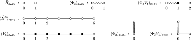
Figure 6.1: The basic graphical units.

Before giving a precise definition of our graphs, we outline how they arise from (6.4). A matrix element $\widehat{H}_{x_{0}x_{1}}$ is represented by two vertices, $0$ and $1$. To each vertex $v$ we assign a label $x_{v}\in\Lambda_{N}$. Matrix multiplication is represented by concatenating such edges. Thus, $\widehat{H}_{x_{0}x_{1}}\cdots\widehat{H}_{x_{n-1}x_{n}}$ is represented as a sequence of vertices $0,\dots,n$ joined by $n$ edges. The root is always the leftmost vertex, and the edges are directed away from the root. If two neighbouring vertices $u,w$ of a vertex $v$ are constrained to have different labels (the nonbacktracking condition), we draw $v$ using a black dot; otherwise, we draw $v$ using a white dot. A factor $\Phi_{2}$ gives rise to a directed edge, represented by a slashed double line, whose final vertex is “dangling” in the sense that it has degree one. A factor $\Phi_{3}$ is represented by a wiggly edge. See Figure 6.1 for an illustration of these rules.

Using these graphical building blocks we may conveniently represent any summand of (6.4). See Figure 6.2 for an example.

Figure 6.2: Graphical representation of the term $V_{2}\,\Phi_{2}\,\Phi_{2}\,\underline{\Phi_{3}V_{2}}\,\Phi_{3}\,\Phi_{3}\,\underline{\Phi_{2}V_{1}}\,\underline{\Phi_{2}V_{2}}\,\underline{\Phi_{3}V_{3}}$.

6.3 Definition of graphs

We now give a precise definition of a set of graphs that is sufficiently general for our purposes. Let $G$ be a finite, oriented, unlabelled, rooted tree. We denote by $\mathcal{V}(G)$ the set of vertices of $G$, by $\mathcal{E}(G)$ the set of edges of $G$, and by $a(G)\in\mathcal{V}(G)$ the root of $G$. That $G$ is oriented means that $G$ is drawn in the plane, and the edges incident to any vertex are ordered. (Thus, each edge $e$ adjacent to a vertex $v$ has a successor, defined as the next edge adjacent to $v$ counting anticlockwise from $e$.) In particular, two graphs are considered different even if they are isomorphic in the usual graph-theoretical sense but the ordering of the edges at some vertex differs. This notion of orientation can be formalized using Dick paths (see e.g. [3], Chapter 1). Such a formal definition is not necessary for our purposes however.

The choice of a root $a(G)$ implies that we may view $G$ as a directed graph, whereby edges are directed away from the root. Thus we shall always regard an edge $e=(v,w)$ as an ordered pair of vertices. Given an edge $e=(v,w)\in\mathcal{E}(G)$, we denote by $a(e)=v$ the initial vertex of $e$ and by $b(e)=w$ the final vertex of $e$.

There is a natural notion of distance between vertices: For $v,w\in\mathcal{V}(G)$ we set $d(v,w)$ to be equal to the number of edges in the shortest path from $v$ to $w$. Each vertex $v\neq a(G)$ has a parent $w$, defined as the unique vertex adjacent to $v$ and satisfying $d(a(G),w)=d(a(G),v)-1$. If $w$ is the parent of $v$ we also say that $v$ is a child of $w$. Similarly, if an edge $e$ is not incident to $a(G)$, we call the (unique) edge $e^{\prime}$ satisfying $a(e)=b(e^{\prime})$ the parent of $e$; in this case we also call $e$ a child of $e^{\prime}$.

We require that $G$ have an additional distinguished vertex $b(G)\in\mathcal{V}(G)$, which need not be different from $a(G)$. The path connecting $a(G)$ to $b(G)$ is called the stem of $G$, and denoted by $\mathcal{S}(G)$. When drawing $G$ in the plane, we draw the stem as a horizontal path from $a(G)$ at its left edge to $b(G)$ at its right edge. We require that all edges not belonging to the stem lie above it (see Figure 6.3). Ultimately, the vertices $a(G)$ and $b(G)$ will receive the fixed labels $x_{a(G)}=x$ and $x_{b(G)}=y$ in the graphical expansion of the matrix element $(U_{n})_{xy}$.

We denote the set of such graphs by $\mathfrak{W}$. We call an edge $e\in\mathcal{E}(G)$ a stem edge if it belongs to $\mathcal{E}(\mathcal{S}(G))$, and a bough edge otherwise. If $G$ has no bough edges, we call it a bare stem. A bare stem is uniquely determined by its number of edges.

Thus, a graph $G\in\mathfrak{W}$ consists of a stem and a collection of rooted trees, called boughs. Each bough is directed away from its root vertex, which belongs to the stem $\mathcal{S}(G)$. We abbreviate with $\mathcal{B}(G)$ the subgraph of $G$ consisting of all bough edges. We call a bough edge $e\in\mathcal{E}(\mathcal{B}(G))=\mathcal{E}(G)\setminus\mathcal{E}(\mathcal{S}(G))$ a leaf if $b(e)$ has degree one. See Figure 6.3 for an example of a graph in $\mathfrak{W}$.

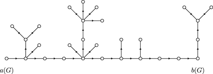
Figure 6.3: A graph in $\mathfrak{W}$.

Next, we decorate graphs $G\in\mathfrak{W}$ as follows. First, we tag the edges, i.e. we choose a map $\tau_{G}$ on $\mathcal{E}(G)$, called a tagging, with values in the set of tags

$$\bigl{\{}{(s,0),(s,1),(b,0),(b,1),(b,2),(b,3),(b,4)}\bigr{\}}\,.$$ (6.7)

Here $s$ stands for “stem” and $b$ for “bough”. We require that the tag $\tau_{G}(e)$ be of the form $(s,i)$ if $e\in\mathcal{E}(\mathcal{S}(G))$ and of the form $(b,i)$ otherwise. The index $i$ (taking values in $\{0,1\}$ for stem edges and $\{0,\dots,4\}$ for bough edges) is used to tag different types of edges. Edges whose tag is $(s,0)$ or $(b,0)$ are called large; other edges are called small. The reason for this nomenclature lies in the magnitude of their contribution to the value of the graph after taking the expectation; see Section 9. Second, we choose a symmetric map $l_{G}:\mathcal{V}(G)^{2}\to\{0,1\}$ which will be used to encode all nonbacktracking conditions on $G$. The idea is that $l_{G}(v,w)=1$ induces a constraint $x_{v}\neq x_{w}$ on the labels. We require that $l(v,w)=0$ unless $d(v,w)=2$. We call the triple $(G,\tau_{G},l_{G})$ a decorated graph, and denote the set of decorated graphs by $\mathfrak{G}$.

Next, we associate a value $\mathfrak{V}_{xy}(\mathcal{G})$ with each decorated graph $\mathcal{G}\in\mathfrak{G}$. The value $\mathfrak{V}_{xy}(\mathcal{G})$ is a random variable that depends on two labels $x,y\in\Lambda_{N}$. For the following we fix $\mathcal{G}=(G,\tau_{G},l_{G})$. We shall assign a label $x_{v}\in\Lambda_{N}$ to each vertex $v\in\mathcal{V}(G)$ in such a way that $x=x_{a(G)}$ and $y=x_{b(G)}$. To define $\mathfrak{V}_{xy}(G)$ we first assign a polynomial in the matrix entries to each edge. Let $e\in\mathcal{E}(G)$ and abbreviate $x_{0}=x_{a(e)}$ and $x_{1}=x_{b(e)}$. We associate a polynomial $P_{\tau_{G}(e)}(\widehat{H}_{x_{0}x_{1}},\widehat{H}_{x_{1}x_{0}})$, and a degree $\deg_{\tau_{G}}(e)\equiv\deg(e)$, with $e$ according to the following table.

$\tau_{G}(e)$	$P_{\tau_{G}(e)}(\widehat{H}_{x_{0}x_{1}},\widehat{H}_{x_{1}x_{0}})$	$\deg(e)$
$(s,0)$	$\widehat{H}_{x_{0}x_{1}}$	$1$
$(s,1)$	$-\lvert\widehat{H}_{x_{0}x_{1}}\rvert^{2}\widehat{H}_{x_{0}x_{1}}$	$3$
$(b,0)$	$\lvert\widehat{H}_{x_{0}x_{1}}\rvert^{2}$	$2$
$(b,1)$	$\lvert\widehat{H}_{x_{0}x_{1}}\rvert^{2}-\sigma^{2}_{x_{0}x_{1}}$	$2$
$(b,2)$, $(b,3)$	$-\lvert\widehat{H}_{x_{0}x_{1}}\rvert^{4}$	$4$
$(b,4)$	$\lvert\widehat{H}_{x_{0}x_{1}}\rvert^{6}$	$6$

Note that $\deg(e)$ is nothing but the degree of the polynomial $P_{\tau_{G}(e)}$. The degree of $\mathcal{G}$ is

$$\deg(\mathcal{G})\;\mathrel{\mathop{:}}=\;\sum_{e\in\mathcal{E}(G)}\deg(e)\,.$$ (6.8)

In order to define $\mathfrak{V}_{xy}(\mathcal{G})$ it is convenient to abbreviate the family of labels by $\bm{\mathrm{x}}=\bigl{(}{x_{v}:v\in\mathcal{V}(G)}\bigr{)}$. Then we set

$$\mathfrak{V}_{xy}(\mathcal{G})\;\mathrel{\mathop{:}}=\;\sum_{\bm{\mathrm{x}}}\delta_{xx_{a(G)}}\delta_{yx_{b(G)}}\Biggl{[}{\prod_{v,w\in\mathcal{V}(G)}\bigl{(}{1-l_{G}(v,w)\delta_{x_{v}x_{w}}}\bigr{)}}\Biggr{]}\Biggl{[}{\prod_{e\in\mathcal{E}(G)}P_{\tau_{G}(e)}\bigl{(}{\widehat{H}_{x_{a(e)}x_{b(e)}},\widehat{H}_{x_{b(e)}x_{a(e)}}}\bigr{)}}\Biggr{]}\,.$$ (6.9)

The summation over $\bm{\mathrm{x}}$ means unrestricted summation for all $x_{v}\in\Lambda_{N}$, $v\in\mathcal{V}(G)$.

We call a stem vertex $v\in\mathcal{V}(\mathcal{S}(G))\setminus\{a(G),b(G)\}$ nonbacktracking if the two stem edges adjacent to $v$, $(u,v)$ and $(v,w)$, satisfy $l_{G}(u,w)=1$; according to (6.9), this means that we have the constraint $x_{u}\neq x_{w}$. Otherwise we call $v$ backtracking. We call the stem $\mathcal{S}(G)$ completely nonbacktracing if all vertices in $\mathcal{V}(\mathcal{S}(G))\setminus\{a(G),b(G)\}$ are nonbacktracking. Decorated graphs $(G,\tau_{G},l_{G})\in\mathfrak{G}$ are represented graphically as follows. Each edge of $G$ is drawn using a decoration that identifies its tag $\tau_{G}(e)$; see Figure 6.4. (Note that, although Figure 6.4 suggests that decorated bough edges are double, they are in fact single. This graphical representation using double lines is chosen in the light of the graph operations $\mathcal{F}_{n}$, $\mathcal{F}_{c}$, and $\mathcal{R}$ defined below.) Non-backtracking stem vertices are drawn with a black dot; other vertices are drawn with a white dot. Note that using black and white dots to draw the vertices displays only partial information about $l_{G}$: Only nonbacktracking restrictions pertaining to pairs of vertices both in the stem are indicated in our graphical representation.

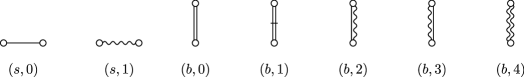
Figure 6.4: The edge decorations along with their associated tags.

See Figure 6.5 for an example of a decorated graph.

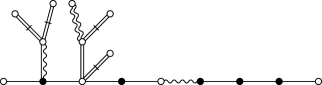
Figure 6.5: A decorated graph in $\mathfrak{G}$.

6.4 Operations on graphs

As it turns out, in order to control the graph expansion we shall have to make all stem vertices apart from $a(G)$ and $b(G)$ nonbacktracking. To this end, we introduce two operations, $\mathcal{F}_{n}$ and $\mathcal{F}_{c}$, on the set of decorated graphs $\mathfrak{G}$. We shall prove that after a finite number of successive applications of either $\mathcal{F}_{n}$ or $\mathcal{F}_{c}$ to an arbitrary decorated graph, we always get a graph with a completely nonbacktracking stem. The index $n$ stands for “nonbacktracking” and $c$ for “collapsing”. The idea behind the definition of $\mathcal{F}_{n}$ and $\mathcal{F}_{c}$ is to choose the first (in the natural order of $\mathcal{S}(G)$) backtracking stem vertex $v_{1}\in\mathcal{V}(\mathcal{S}(G))\setminus\{a(G),b(G)\}$ and introduce a splitting in the definition (6.9) using

$$1\;=\;\bm{\mathrm{1}}(x_{v_{0}}\neq x_{v_{2}})+\bm{\mathrm{1}}(x_{v_{0}}=x_{v_{2}})\,,$$

where the vertices $v_{0},v_{2}\in\mathcal{V}(\mathcal{S}(G))$ are the neighbours of $v_{1}$ in the stem, i.e. they satisfy $(v_{0},v_{1}),(v_{1},v_{2})\in\mathcal{E}(\mathcal{S}(G))$.

We now define $\mathcal{F}_{n}$ and $\mathcal{F}_{c}$ more precisely. If $\mathcal{S}(G)$ has no backtracking vertex, set $\mathcal{F}_{n}(\mathcal{G})\mathrel{\mathop{:}}=\mathcal{G}$ and $\mathcal{F}_{c}(\mathcal{G})\mathrel{\mathop{:}}=\emptyset$, where $\emptyset$ is the empty graph satisfying $\mathfrak{V}_{xy}(\emptyset)\mathrel{\mathop{:}}=0$.

Otherwise, let $v_{1}$ be the first backtracking vertex in $\mathcal{V}(\mathcal{S}(G))\setminus\{a(G),b(G)\}$ and define $v_{0}$ and $v_{2}$ as above. Then we set $\mathcal{F}_{n}(\mathcal{G})\mathrel{\mathop{:}}=(G,\tau_{G},\widetilde{l}_{G})$, where

$$\widetilde{l}_{G}(v,w)\;\mathrel{\mathop{:}}=\;l_{G}(v,w)+\delta_{vv_{0}}\delta_{wv_{2}}+\delta_{wv_{0}}\delta_{vv_{2}}\,.$$

Thus, the operation $\mathcal{F}_{n}$ simply makes the vertex $v_{1}$ a nonbacktracking vertex of $\mathcal{S}(G)$ without changing $G$ or $\tau_{G}$, i.e. it sets $\widetilde{l}_{G}(v_{0},v_{2})=\widetilde{l}_{G}(v_{2},v_{0})=1$ and leaves $\widetilde{l}_{G}$ unchanged for any other pair of vertices.

Next, we define $\mathcal{F}_{c}$. Let $v_{0},v_{1},v_{2}$ be as above. The operation $\mathcal{F}_{c}$ collapses the two nearest stem neighbours, $v_{0}$ and $v_{2}$, of $v_{1}$ into one vertex and fuses the two edges $(v_{0},v_{1})$ and $(v_{1},v_{2})$ into one edge (see Figure 6.6). This definition is very natural in the light of Figure 6.6 and our choice of conventions for drawing bough edges as double lines. Thus, a reader who believes his eyes when gazing at pictures like Figure 6.6 may safely skip the following two paragraphs.

To define the operation $\mathcal{F}_{c}$ precisely, we identify $v_{0}$ with $v_{2}$, i.e. introduce the equivalence classes

$$[v]\;\mathrel{\mathop{:}}=\;\begin{cases}\{v\}&\text{if }v\notin\{v_{0},v_{2}\}\\ \{v_{0},v_{2}\}&\text{if }v\in\{v_{0},v_{2}\}\,.\end{cases}$$

Define the graph $\widetilde{G}$ through its vertex set $\mathcal{V}(\widetilde{G})=\{[v]\,:\,v\in\mathcal{V}(G)\}$, and its edge set, which is obtained as follows. Each edge $(v,w)\in\mathcal{E}(G)\setminus\{(v_{1},v_{2})\}$ gives rise to the edge $([v],[w])\in\mathcal{E}(\widetilde{G})$. Thus, the edges $(v_{0},v_{1})$ and $(v_{1},v_{2})$ are fused into a single edge $([v_{0}],[v_{1}])$. The tag $\tau_{\widetilde{G}}\bigl{(}{([v],[w])}\bigr{)}$ is by definition equal to the tag $\tau_{G}\bigl{(}{(v,w)}\bigr{)}$ if $(v,w)\neq(v_{0},v_{1})$; the tag of the edge $([v_{0}],[v_{1}])$ is defined by the following table.

$\tau_{G}\bigl{(}{(v_{0},v_{1})}\bigr{)}$	$\tau_{G}\bigl{(}{(v_{1},v_{2})}\bigr{)}$	$\tau_{\widetilde{G}}\bigl{(}{([v_{0}],[v_{1}])}\bigr{)}$
$(s,0)$	$(s,0)$	$(b,0)$
$(s,0)$	$(s,1)$	$(b,2)$
$(s,1)$	$(s,0)$	$(b,3)$
$(s,1)$	$(s,1)$	$(b,4)$

The initial and final vertices of $\widetilde{G}$ are given by $a(\widetilde{G})\mathrel{\mathop{:}}=[a(G)]$ and $b(\widetilde{G})\mathrel{\mathop{:}}=[b(G)]$. The edges of $\widetilde{G}$ are oriented in the natural way when drawing $G$ and $\widetilde{G}$ in the plane; instead of giving a formal definition of the orientation, we refer to Figure 6.6.

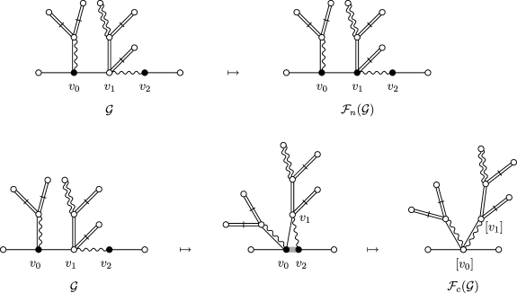
Figure 6.6: Graphical representation of the operations $\mathcal{F}_{n}$ and $\mathcal{F}_{c}$.

Finally, we define the map $l_{\widetilde{G}}$, which encodes the nonbacktracking information of $\widetilde{G}$, through

$$l_{\widetilde{G}}(\widetilde{v},\widetilde{w})\;\mathrel{\mathop{:}}=\;\begin{cases}1&l_{G}(v,w)=1\text{ for some pair of representatives }v\in\widetilde{v},w\in\widetilde{w}\\ 0&\text{otherwise}\,.\end{cases}$$

Thus, in the graphical representation of $\mathcal{F}_{c}(\mathcal{G})\mathrel{\mathop{:}}=(\widetilde{G},\tau_{\widetilde{G}},l_{\widetilde{G}})$, the vertex $[v_{0}]=[v_{2}]$ is always white (i.e. backtracking). Note that if $v_{0}$ or $v_{2}$ was nonbacktracking, this restriction remains encoded in the map $l_{\widetilde{G}}$, but is no longer visible in the colouring of the vertices.

We summarize the key properties of $\mathcal{F}_{n}$ and $\mathcal{F}_{c}$, which follow immediately from their construction.

Lemma 6.3.

Let $\mathcal{G}\in\mathfrak{G}$. Then $\mathcal{F}_{n}(\mathcal{G}),\mathcal{F}_{c}(\mathcal{G})\in\mathfrak{G}$. Moreover,

$$\mathfrak{V}_{xy}(\mathcal{G})\;=\;\mathfrak{V}_{xy}(\mathcal{F}_{n}(\mathcal{G}))+\mathfrak{V}_{xy}(\mathcal{F}_{c}(\mathcal{G}))\,,$$

and

$$\deg(\mathcal{F}_{n}(\mathcal{G}))\;=\;\deg(\mathcal{F}_{c}(\mathcal{G}))\;=\;\deg(\mathcal{G})\,.$$

6.5 Graphs with completely nonbacktracking stem

Next, we introduce two special subsets of decorated graphs. We define $\mathfrak{G}^{\prime}\subset\mathfrak{G}$ to be the set of decorated graphs corresponding to terms in (6.4). See Figure 6.2 for an example. More precisely:

Definition 6.4.

The set $\mathfrak{G}^{\prime}$ is the subset of $(G,\tau_{G},l_{G})\in\mathfrak{G}$ satisfying

1. All boughs of $G$ contain only one edge, whose tag is $(b,1)$;

2. $l_{G}(u,w)=1$ if and only if there is a vertex $v$ that is not the root of a bough, such that $(u,v),(v,w)\in\mathcal{E}(\mathcal{S}(G))$ with $\tau_{G}\bigl{(}{(v,w)}\bigr{)}=(s,0)$.

Property (ii) says that all bough vertices (including the bough roots) are white, and that the left vertex of a wiggly edge is white. The remaining vertices (apart from $a(G)$ and $b(G)$) are black. It is easy to see that the graphs associated with terms on the right-hand side of (6.4) belong to $\mathfrak{G}^{\prime}$

Note that, unlike in the case of a general graph $\mathcal{G}\in\mathfrak{G}$, the nonbacktracking information of a graph $\mathcal{G}\in\mathfrak{G}^{\prime}$ is fully encoded in the colouring of its vertices. Indeed, $l_{G}(v,w)$ can only be $1$ if $v,w\in\mathcal{V}(\mathcal{S}(G))$. Moreover, from (ii) we see that $l_{G}$ is uniquely determined by $G$ and $\tau_{G}$. Thus, a decorated graph $\mathcal{G}=(G,\tau_{G},l_{G})\in\mathfrak{G}^{\prime}$ is uniquely determined by its graph and tagging, i.e. the pair $(G,\tau_{G})$.

The second important subset of decorated graphs is generated from $\mathfrak{G}^{\prime}$ by applying the operations $\mathcal{F}_{n},\mathcal{F}_{c}$ to decorated graphs in $\mathfrak{G}^{\prime}$ until the stem is completely nonbacktracking, i.e. all stem vertices (apart from $a(G)$ and $b(G)$) are black.

Definition 6.5.

For $\mathcal{G}\in\mathfrak{G}^{\prime}$ we define $\mathscr{B}_{\mathcal{G}}$ as the set of decorated graphs $\widetilde{\mathcal{G}}\in\mathfrak{G}$ whose stem is completely nonbacktracking and that are obtained from $\mathcal{G}$ by a finite number of operations $\mathcal{F}_{n}$ and $\mathcal{F}_{c}$. Furthermore we set

$$\mathfrak{G}_{\sharp}\;\mathrel{\mathop{:}}=\;\bigcup_{\mathcal{G}\in\mathfrak{G}^{\prime}}\mathscr{B}_{\mathcal{G}}\,.$$

The set $\mathfrak{G}_{\sharp}$ is the set of “good” graphs that we shall work with in later sections. Thus, given a graph $\mathcal{G}\in\mathfrak{G}^{\prime}$ corresponding to a summand of (6.4), we first transform it into the family $\mathscr{B}_{\mathcal{G}}$ of graphs in $\mathfrak{G}_{\sharp}$. The contribution of $\mathcal{G}$ to the expansion (6.4) is given by the sum of the contributions of all graphs in $\mathscr{B}_{\mathcal{G}}$ (see (6.10) below). We then exploit the fact that we have good estimates on the contributions of graphs with completely nonbacktracking stems.

Next, we state and prove the key properties of the set $\mathfrak{G}_{\sharp}$ and the operations $\mathcal{F}_{n}$ and $\mathcal{F}_{c}$.

Proposition 6.6.

1. If $\mathcal{G}=(G,\tau_{G},l_{G})\in\mathfrak{G}_{\sharp}$ then $l_{G}$ is uniquely determined by the pair $(G,\tau_{G})$ alone. In other words, there is a function $\ell$ such that $l_{G}=\ell(G,\tau_{G})$ for all $(G,\tau_{G},l_{G})\in\mathfrak{G}_{\sharp}$.

2. If $(G,\tau_{G},l_{G})\in\mathfrak{G}_{\sharp}$ then all leaves of $G$ are small (in $\tau_{G}$).

3. If $(G,\tau_{G},l_{G})\in\mathfrak{G}_{\sharp}$ and $e\in\mathcal{E}(G)$ has tag $\tau_{G}(e)=(b,1)$, then $e$ is a leaf of $G$.

4. If $\mathcal{G}\neq\mathcal{G}^{\prime}\in\mathfrak{G}^{\prime}$ then $\mathscr{B}_{\mathcal{G}}\cap\mathscr{B}_{\mathcal{G}^{\prime}}=\emptyset$.

5. For any $\mathcal{G}\in\mathfrak{G}^{\prime}$ and $\widetilde{\mathcal{G}}\in\mathscr{B}_{\mathcal{G}}$ we have $\deg(\mathcal{G})=\deg(\widetilde{\mathcal{G}})$.

6. For each $\mathcal{G}\in\mathfrak{G}^{\prime}$ we have

   $$\mathfrak{V}_{xy}(\mathcal{G})\;=\;\sum_{\widetilde{\mathcal{G}}\in\mathscr{B}_{\mathcal{G}}}\mathfrak{V}_{xy}(\widetilde{\mathcal{G}})\,.$$ (6.10)

Proof.

The key ingredient of the proof is the following ripping operation, denoted by $\mathcal{R}$. It provides a link between the sets $\mathfrak{G}_{\sharp}$ and $\mathfrak{G}^{\prime}$, and is essentially the converse of multiple applications of $\mathcal{F}_{n}$ and $\mathcal{F}_{c}$. The idea is to take hold of the vertices $a(G)$ and $b(G)$ of a given tagged graph $(G,\tau_{G})$ and “pull them apart”, thus “ripping open” all bough edges of $\mathcal{G}$ except those of type $(b,1)$. When interpreted graphically, the character of each edge (straight or wiggly) is kept unchanged, whereby the double edge of a bough edge is split into two single edges.

When defining $\mathcal{R}$ it is convenient, in a first step, to “rip open” all bough edges (including those of type $(b,1)$) of $(G,\tau_{G})$; we shall call the resulting tagged graph $\mathcal{P}(G,\tau_{G})$. In a second step, we undo the ripping of all bough edges of type $(b,1)$, which results in the tagged graph $\mathcal{R}(G,\tau_{G})$.

In order to define $\mathcal{P}$, we need one additional tag $(s,2)$ for stem edges, which we draw with a single solid line that is slashed. Stem edges of type $(s,2)$ result from the ripping open of a bough edge of type $(b,1)$. By walking around $G$, we associate with the tagged graph $(G,\tau_{G})$ a tagged bare stem $(\widetilde{G},\tau_{\widetilde{G}})=\mathrel{\mathop{:}}\mathcal{P}(G,\tau_{G})$. More precisely, we draw $G$ in the plane, and start at the vertex $a(G)$. At each step, we move along one edge of $G$ in such a way that we always remain to the left of $G$; see Figure 6.7. Every stem edge is travelled once, and every bough edge twice. Each time we move along an edge $e\in\mathcal{E}(G)$, we add an edge $\widetilde{e}$ to the stem $\widetilde{G}$. Depending on whether we moved along $e$ in the direction of $e$ (denoted by $+$) or against the direction of $e$ (denoted by $-$), we associate a tag $\tau_{\widetilde{G}}(\widetilde{e})$ with $\widetilde{e}$ according to the following table.

$\tau_{G}(e)$	direction	$\tau_{\widetilde{G}}(\widetilde{e})$
$(s,0)$	$+$	$(s,0)$
$(s,1)$	$+$	$(s,1)$
$(b,0)$	$\pm$	$(s,0)$
$(b,1)$	$\pm$	$(s,2)$
$(b,2)$	$+$	$(s,0)$
$(b,2)$	$-$	$(s,1)$
$(b,3)$	$+$	$(s,1)$
$(b,3)$	$-$	$(s,0)$
$(b,4)$	$\pm$	$(s,1)$

Graphical representation of $(s,2)$:  

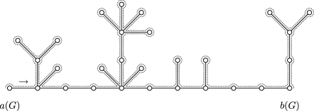
Figure 6.7: The walk around $G$.

These rules are made obvious by a glance at Figure 6.4; indeed, a tagged bough edge is represented with a double line which corresponds exactly to the two single lines resulting from ripping the bough edge open. Figure 6.9 provides an example of the operation $(G,\tau_{G})\mapsto\mathcal{P}(G,\tau_{G})$. The map $\mathcal{P}$ can also be interpreted as first doubling all bough edges according to their tags, and ripping them open successively by pulling the edges $a(G)$ and $b(G)$ apart; see Figure 6.8.

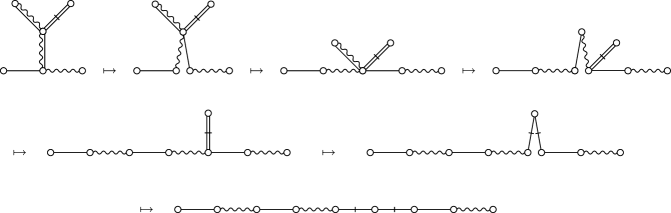
Figure 6.8: The dynamical process of successively ripping open doubled bough edges. Note that the stem edges with tag $(s,2)$ (drawn with a slashed single line) always occur in consecutive pairs.

We now define $\mathcal{R}(G,\tau_{G})=\mathcal{G}^{\prime}$ to be the unique decorated graph $\mathcal{G}^{\prime}=(G^{\prime},\tau_{G^{\prime}},l_{G^{\prime}})\in\mathfrak{G}^{\prime}$ that satisfies $\mathcal{P}(G,\tau_{G})=\mathcal{P}(G^{\prime},\tau_{G^{\prime}})$; see Figure 6.9. That there is exactly one such $\mathcal{G}^{\prime}\in\mathfrak{G}^{\prime}$ follows immediately from the definitions of $\mathcal{P}$ and $\mathfrak{G}^{\prime}$, as well as the fact that $l_{G^{\prime}}$ is uniquely determined by the pair $(G^{\prime},\tau_{G^{\prime}})$ through Definition 6.4 (ii). (Thus, the operation $\mathcal{P}$ plays only an auxiliary role, its sole purpose being to clarify the definition of $\mathcal{R}$.)

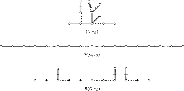
Figure 6.9: The definitions of $\mathcal{P}$ and $\mathcal{R}$.

Having defined the ripping operation $\mathcal{R}$, we are now ready to prove Claim (i) of the Proposition. Before giving the full proof we outline the strategy. First, for any $\mathcal{G}=(G,\tau_{G},l_{G})\in\mathfrak{G}_{\sharp}$ we construct the ripped graph $\mathcal{R}(G,\tau_{G})\in\mathfrak{G}^{\prime}$, which does not depend on $l_{G}$. Second, by definition of $\mathfrak{G}^{\prime}$, the ripped graph $\mathcal{G}^{\prime}=\mathcal{R}(G,\tau_{G})$ bears a unique nonbacktracing map $l_{G^{\prime}}$. Third, by definition of $\mathfrak{G}_{\sharp}$, there is a sequence $i_{1},\dots,i_{k}\in\{n,c\}$ such that $\mathcal{G}=(G,\tau_{G},l_{G})=(\mathcal{F}_{i_{k}}\circ\cdots\circ\mathcal{F}_{i_{1}})(\mathcal{R}(G,\tau_{G}))$. Fourth, we prove that this representation is unique. Thus we have expressed $l_{G}$ as a function of $(G,\tau_{G})$.

Now to the proof of (i). Let $\mathcal{G}=(G,\tau_{G},l_{G})\in\mathfrak{G}_{\sharp}$. By definition of $\mathfrak{G}_{\sharp}$, there is a decorated graph $\mathcal{G}^{\prime}=(G^{\prime},\tau_{G^{\prime}},l_{G^{\prime}})\in\mathfrak{G}^{\prime}$ and a finite sequence $i_{1},\dots,i_{k}\in\{n,c\}$ such that

$$\mathcal{G}\;=\;\bigl{(}{\mathcal{F}_{i_{k}}\circ\cdots\circ\mathcal{F}_{i_{1}}}\bigr{)}(\mathcal{G}^{\prime})\,.$$ (6.11)

We now claim that both $\mathcal{G}^{\prime}$ and the sequence $i_{1},\dots,i_{k}$ are uniquely determined by $(G,\tau_{G})$ (under the obvious constraint that no $\mathcal{F}_{i_{j}}$ is allowed to act on a decorated graph whose stem is completely nonbacktracking). Indeed, we must have that $\mathcal{G}^{\prime}=\mathcal{R}(G,\tau_{G})$. (This follows immediately from the fact that $\mathcal{R}$ is left invariant under the action of $\mathcal{F}_{i}$, $i\in\{n,c\}$; i.e. $\mathcal{R}(G_{2},\tau_{G_{2}})=\mathcal{R}(G_{1},\tau_{G_{1}})$ for any $(G_{2},\tau_{G_{2}},l_{G_{2}})=\mathcal{F}_{i}(G_{1},\tau_{G_{1}},l_{G_{1}})$ where $(G_{1},\tau_{G_{1}},l_{G_{1}})\in\mathfrak{G}$.)

That different (under the above constraint) sequences applied to $\mathcal{R}(G,\tau_{G})$ yield a different tagged graph is an immediate consequence of the following general claim. In order to state it, we introduce the set $\mathscr{D}_{\widetilde{\mathcal{G}}}$ as the set of decorated graphs obtained from $\widetilde{\mathcal{G}}\in\mathfrak{G}$ by a arbitrary applications of the operations $\mathcal{F}_{n},\mathcal{F}_{c}$. (The set $\mathscr{D}_{\widetilde{\mathcal{G}}}$ will be used in the statement and the proof of the following Claim $(*)$. We remark that the previously defined set $\mathscr{B}_{\widetilde{\mathcal{G}}}$ is a subset of $\mathscr{D}_{\widetilde{\mathcal{G}}}$ with the additional requirement that the stem is black.)

• Let $\widetilde{\mathcal{G}}=(\widetilde{G},\tau_{\widetilde{G}},l_{\widetilde{G}})\in\mathfrak{G}$ be an arbitrary decorated graph whose stem is not completely nonbacktracking. Then for any $\mathcal{G}_{1}=(G_{1},\tau_{G_{1}},l_{G_{1}})\in\mathscr{D}_{\mathcal{F}_{n}(\widetilde{\mathcal{G}})}$ and $\mathcal{G}_{2}=(G_{2},\tau_{G_{2}},l_{G_{2}})\in\mathscr{D}_{\mathcal{F}_{c}(\widetilde{\mathcal{G}})}$ we have $G_{1}\neq G_{2}$.

Claim $(*)$ will be used in the following situation. We shall apply sequences of operations $\mathcal{F}_{n}$ and $\mathcal{F}_{c}$ to a decorated graph $\mathcal{G}^{\prime}\in\mathfrak{G}^{\prime}$. If two sequences of such operations differ from each other in at least one step, then the resulting two graphs will be different. In other words, if a decorated graph $\mathcal{G}$ can be written in the form (6.11) and $\mathcal{G}^{\prime}$ is known, then the sequence $i_{1},i_{2},\dots,i_{k}$ is uniquely determined. Together with the uniqueness of $\mathcal{G}^{\prime}=\mathcal{R}(G,\tau_{G})$ established earlier, this proves the uniqueness of the representation (6.11). Thus we can define the map $\ell:(G,\tau_{G})\to l_{G}$ through

$$\mathcal{G}\;=\;(G,\tau_{G},l_{G})\;=\;\bigl{(}{\mathcal{F}_{i_{k}}\circ\cdots\circ\mathcal{F}_{i_{1}}}\bigr{)}\bigl{(}{\mathcal{R}(G,\tau_{G})}\bigr{)}\,,$$

and hence Claim (i) follows.

We now prove Claim $(*)$. For any graph $\widetilde{G}\in\mathfrak{W}$ and integer $q\in Q_{\widetilde{G}}\mathrel{\mathop{:}}=\bigl{\{}{0,1,\dots,\lvert\mathcal{E}(\mathcal{S}(\widetilde{G}))\rvert+2\lvert\mathcal{E}(\mathcal{B}(\widetilde{G}))\rvert}\bigr{\}}$, we define the vertex $v_{\widetilde{G}}(q)\in\mathcal{V}(\widetilde{G})$ as the vertex reached after $q$ steps of the walk around $\widetilde{G}$ (see Figure 6.7). For $q\in Q_{\widetilde{G}}$ we define the “time of next return” $r_{\widetilde{G}}(q)$ as the smallest integer $q^{\prime}>q$ such that $v_{\widetilde{G}}(q^{\prime})=v_{\widetilde{G}}(q)$; if there is no such $q^{\prime}$, we set $q^{\prime}\mathrel{\mathop{:}}=\infty$.

Next, let $v_{1}\in\mathcal{V}(\widetilde{G})\setminus\{a(\widetilde{G}),b(\widetilde{G})\}$ be the first backtracking stem vertex of $\widetilde{G}$, and denote by $v_{0}$ its parent vertex (for an example see Figure 6.6). Define $q_{0}$ as the “last time we walk across $v_{0}$”, i.e. as the largest integer in $Q_{\widetilde{G}}$ satisfying $v_{\widetilde{G}}(q_{0})=v_{0}$. By definition of $q_{0}$, we have $r_{\widetilde{G}}(q_{0})=\infty$. Now define $\mathcal{G}_{c}=(G_{c},\tau_{G_{c}},l_{G_{c}})\mathrel{\mathop{:}}=\mathcal{F}_{c}(\widetilde{\mathcal{G}})$. Clearly, we have that $r_{G_{c}}(q_{0})<\infty$. Moreover, one readily sees that

$$r_{G_{2}}(q_{0})\;=\;r_{G_{c}}(q_{0})\;<\;r_{G_{1}}(q_{0})\,,$$ (6.12)

for all $\mathcal{G}_{1}=(G_{1},\tau_{G_{1}},l_{G_{1}})\in\mathscr{D}_{\mathcal{F}_{n}(\widetilde{\mathcal{G}})}$ and $\mathcal{G}_{2}=(G_{2},\tau_{G_{2}},l_{G_{2}})\in\mathscr{D}_{\mathcal{F}_{c}(\widetilde{\mathcal{G}})}$. The equality expresses the fact that $v_{0}$ and $v_{2}$ have already been collapsed into one vertex in all $\mathcal{G}_{2}\in\mathscr{D}_{\mathcal{F}_{c}(\widetilde{\mathcal{G}})}$. The inequality expresses the fact that, while $v_{0}$ may be collapsed with a stem vertex $v_{j}$ at some point when constructing $G_{1}\in\mathscr{D}_{\mathcal{F}_{n}(\widetilde{\mathcal{G}})}$, the walk from $v_{0}$ to $v_{j}$ is strictly longer than from $v_{0}$ to $v_{2}$. Claim $(*)$ follows immediately from (6.12).

Next, we prove Claim (ii). If $\mathcal{G}\in\mathfrak{G}^{\prime}$ then by definition all leaf edges have tag $(b,1)$, i.e. are small. This also holds for $\mathcal{F}_{n}(\mathcal{G})$ (trivially), as well as for $\mathcal{F}_{c}(\mathcal{G})$. In order to see this, define the property $(\mathrm{P}_{\mathcal{G}})$ as follows.

• If a vertex $v\in\mathcal{V}(G)$ that is not the root of a bough satisfies $(u,v),(v,w)\in\mathcal{E}(\mathcal{S}(G))$ for some vertices $v,w$ and if the tags of $(u,v)$ and $(v,w)$ are both $(s,0)$, then the vertex $v$ is a nonbacktracking stem vertex.

Property $(\mathrm{P}_{\mathcal{G}})$ for a decorated graph $\mathcal{G}$ means that a vertex between two straight stem edges is black unless it is the root of a bough. It is easy to see that the property $(\mathrm{P}_{\mathcal{G}})$ satisfied for all $\mathcal{G}\in\mathfrak{G}^{\prime}$ (see Definition 6.4 (ii)). Moreover, $(\mathrm{P}_{\mathcal{G}})$ is invariant under $\mathcal{F}_{c}$ and $\mathcal{F}_{n}$. Recalling the definition of $\mathfrak{G}_{\sharp}$, we see that Claim (ii) follows by induction.

Next, Claim (iii) clearly holds if $\mathcal{G}=(G,\tau_{G},l_{G})\in\mathfrak{G}^{\prime}$. Moreover, by definition of $\mathcal{F}_{n}$ and $\mathcal{F}_{c}$, Claim (iii) holds for $\mathcal{F}_{n}(\mathcal{G})$ and $\mathcal{F}_{c}(\mathcal{G})$ if it holds for $\mathcal{G}$. Hence Claim (iii) follows from the definition of $\mathfrak{G}_{\sharp}$.

Claim (iv) is an immediate consequence of the fact that if $\widetilde{\mathcal{G}}\in\mathscr{B}_{\mathcal{G}}$ then $\mathcal{G}=\mathcal{R}(\widetilde{\mathcal{G}})$.

Claim (v) is an immediate consequence of the fact that, by definition of $\mathcal{F}_{n}$ and $\mathcal{F}_{c}$, we have $\deg(\mathcal{G})=\deg(\mathcal{F}_{n}(\mathcal{G}))=\deg(\mathcal{F}_{c}(\mathcal{G}))$.

Finally, we prove Claim (vi). Let $\mathcal{G}\in\mathfrak{G}^{\prime}$. Using Lemma 6.3 repeatedly, we get

$$\mathfrak{V}_{xy}(\mathcal{G}) \;=\;\mathfrak{V}_{xy}\bigl{(}{\mathcal{F}_{n}(\mathcal{G})}\bigr{)}+\mathfrak{V}_{xy}\bigl{(}{\mathcal{F}_{c}(\mathcal{G})}\bigr{)}$$

$$\;=\;\mathfrak{V}_{xy}\bigl{(}{\mathcal{F}_{n}(\mathcal{F}_{n}(\mathcal{G}))}\bigr{)}+\mathfrak{V}_{xy}\bigl{(}{\mathcal{F}_{c}(\mathcal{F}_{n}(\mathcal{G}))}\bigr{)}+\mathfrak{V}_{xy}\bigl{(}{\mathcal{F}_{n}(\mathcal{F}_{c}(\mathcal{G}))}\bigr{)}+\mathfrak{V}_{xy}\bigl{(}{\mathcal{F}_{c}(\mathcal{F}_{c}(\mathcal{G}))}\bigr{)}$$

$$\;=\;\dots\;=\;\sum_{i\in I}\mathfrak{V}_{xy}(\mathcal{G}_{i})\,,$$

where $(\mathcal{G}_{i})_{i\in I}$ is a finite family of decorated graphs whose stems are completely nonbacktracking. By definition of $\mathscr{B}_{\mathcal{G}}$, we have $\mathscr{B}_{\mathcal{G}}\;=\;\{{\mathcal{G}_{i}\,:\,i\in I}\}$. What remains is to show that each $\widetilde{\mathcal{G}}\in\mathscr{B}_{\mathcal{G}}$ appears only once in $(\mathcal{G}_{i})_{i\in I}$. But this is an immediate consequence of the uniqueness of the sequence $i_{1},\dots,i_{k}$ in the representation $\widetilde{\mathcal{G}}=\bigl{(}{\mathcal{F}_{i_{k}}\circ\cdots\circ\mathcal{F}_{i_{1}}}\bigr{)}(\mathcal{G})$; see the proof of Claim (i) above. ∎

In view of Proposition 6.6 (i), we may regard the set $\mathfrak{G}_{\sharp}$ as a set of tagged graphs $(G,\tau_{G})$. We shall consistently adopt this point of view from now on.

Proposition 6.7.

We have

$$(U_{n})_{xy}\;=\;\sum_{\mathcal{G}\in\mathfrak{G}^{\prime}\,:\,\deg(\mathcal{G})=n}\mathfrak{V}_{xy}(G)\;=\;\sum_{\mathcal{G}\in\mathfrak{G}_{n}}\mathfrak{V}_{xy}(\mathcal{G})\,,$$ (6.13)

where $\mathfrak{V}_{xy}(\mathcal{G})$ is defined in (6.9), and we defined the subset of graphs

$$\mathfrak{G}_{n}\;\mathrel{\mathop{:}}=\;\bigl{\{}{\mathcal{G}\in\mathfrak{G}_{\sharp}\,:\,\deg(\mathcal{G})=n}\bigr{\}}\,.$$

Proof.

The first equality of (6.13) follows from (6.4) and the definition of $\mathfrak{G}^{\prime}$ (see Definition 6.4); the second from Proposition 6.6 (iv), (v), and (vi). ∎

7 Lumping of edges

Recall that our aim is to compute

$$\widehat{\varrho}_{\leqslant}(t,x)\;=\;\sum_{n+n^{\prime}\leqslant M^{\mu}}\alpha_{n}(t)\,\overline{\alpha_{n^{\prime}}(t)}\!\,\;\mathbb{E}\,(U_{n})_{0x}(U_{n^{\prime}})_{x0}\,.$$

By (6.13) we have

$$\widehat{\varrho}_{\leqslant}(t,x)\;=\;\sum_{n+n^{\prime}\leqslant M^{\mu}}\alpha_{n}(t)\,\overline{\alpha_{n^{\prime}}(t)}\!\,\;\sum_{\mathcal{G}\in\mathfrak{G}_{n}}\sum_{\mathcal{G}^{\prime}\in\mathfrak{G}_{n^{\prime}}}\mathbb{E}\mathfrak{V}_{0x}(\mathcal{G})\mathfrak{V}_{x0}(\mathcal{G}^{\prime})\,.$$ (7.1)

Computing the expectation $\mathbb{E}\mathfrak{V}_{0x}(G)\mathfrak{V}_{x0}(G^{\prime})$ yields a lumping of the edges $\mathcal{E}(G)\cup\mathcal{E}(G^{\prime})$, which we now describe.

For the following we fix $\mathcal{G}=(G,\tau_{G})\in\mathfrak{G}_{\sharp}$ and $\mathcal{G}^{\prime}=(G^{\prime},\tau_{G^{\prime}})\in\mathfrak{G}_{\sharp}$. Thus, we also fix the maps $l_{G}$ and $l_{G^{\prime}}$; see Proposition 6.6 (i). To streamline notation, we introduce their union $\mathcal{G}\cup\mathcal{G}^{\prime}=(G\cup G^{\prime},\tau_{G\cup G^{\prime}})$ defined in the obvious way. We also get the map $l_{G\cup G^{\prime}}$ that we extend by requiring that $l_{G\cup G^{\prime}}(v,w)=0$ if $v\in\mathcal{V}(G)$ and $w\in\mathcal{V}(G^{\prime})$. We often abbreviate $\tau\equiv\tau_{G\cup G^{\prime}}$ and $l\equiv l_{G\cup G^{\prime}}$.

As in the previous section, we abbreviate the family of labels with

$$\bm{\mathrm{x}}\;=\;\bigl{(}{x_{v}\,:\,v\in\mathcal{V}(G\cup G^{\prime})}\bigr{)}\,.$$

From (6.9) we immediately get

$$\mathfrak{V}_{0x}(\mathcal{G})\mathfrak{V}_{x0}(\mathcal{G}^{\prime})\;=\;\sum_{\bm{\mathrm{x}}}\delta_{0x_{a(G)}}\delta_{xx_{b(G)}}\delta_{xx_{a(G^{\prime})}}\delta_{0x_{b(G^{\prime})}}\Biggl{[}{\prod_{v,w\in\mathcal{V}(G\cup G^{\prime})}\bigl{(}{1-l(v,w)\delta_{x_{v}x_{w}}}\bigr{)}}\Biggr{]}\\ \times\prod_{e\in\mathcal{E}(G\cup G^{\prime})}P_{\tau(e)}\bigl{(}{\widehat{H}_{x_{a(e)}x_{b(e)}},\widehat{H}_{x_{b(e)}x_{a(e)}}}\bigr{)}\,.$$ (7.2)

Next, for any fixed $\bm{\mathrm{x}}$ we assign to each edge $e\in\mathcal{E}(G\cup G^{\prime})$ the unordered pair of labels

$$\varrho_{\bm{\mathrm{x}}}(e)\;\mathrel{\mathop{:}}=\;\{x_{a(e)},x_{b(e)}\}\,.$$

To each label configuration $\bm{\mathrm{x}}$ we assign a lumping $\Gamma(\bm{\mathrm{x}})$ of the edges $\mathcal{E}(G\cup G^{\prime})$ according to the value of the map $\varrho_{\bm{\mathrm{x}}}$. We use the word lumping to mean an equivalence relation on $\mathcal{E}(G\cup G^{\prime})$, or, equivalently, a partition of $\mathcal{E}(G\cup G^{\prime})$. More precisely, the lumping $\Gamma(\bm{\mathrm{x}})$ is defined as the equivalence relation (denoted by $\sim$) on $\mathcal{E}(G\cup G^{\prime})$ such that $e\sim e^{\prime}$ if and only if $\varrho_{\bm{\mathrm{x}}}(e)=\varrho_{\bm{\mathrm{x}}}(e^{\prime})$. We use the notation $\Gamma=\{\gamma\}_{\gamma\in\Gamma}$, where $\gamma\subset\mathcal{E}(G\cup G^{\prime})$ is a lump, i.e. an equivalence class. Thus, taking the expectation in (7.2) yields

$$\mathbb{E}\mathfrak{V}_{0x}(\mathcal{G})\mathfrak{V}_{x0}(\mathcal{G}^{\prime})\;=\;\sum_{\bm{\mathrm{x}}}\delta_{0x_{a(G)}}\delta_{xx_{b(G)}}\delta_{xx_{a(G^{\prime})}}\delta_{0x_{b(G^{\prime})}}\Biggl{[}{\prod_{v,w\in\mathcal{V}(G\cup G^{\prime})}\bigl{(}{1-l(v,w)\delta_{x_{v}x_{w}}}\bigr{)}}\Biggr{]}\\ \times\prod_{\gamma\in\Gamma(\bm{\mathrm{x}})}\mathbb{E}\prod_{e\in\gamma}P_{\tau(e)}\bigl{(}{\widehat{H}_{x_{a(e)}x_{b(e)}},\widehat{H}_{x_{b(e)}x_{a(e)}}}\bigr{)}\,,$$ (7.3)

where we used that $\widehat{H}_{a(e)b(e)}$ and $\widehat{H}_{a(e^{\prime})b(e^{\prime})}$ are independent if $\varrho_{\bm{\mathrm{x}}}(e)\neq\varrho_{\bm{\mathrm{x}}}(e^{\prime})$.

Next, we define the indicator function

$$\Delta_{\Gamma}(\bm{\mathrm{x}})\;\mathrel{\mathop{:}}=\;\bm{\mathrm{1}}(\Gamma(\bm{\mathrm{x}})=\Gamma)\;=\;\Biggl{[}{\prod_{\gamma\neq\gamma^{\prime}\in\Gamma}\prod_{e\in\gamma}\prod_{e^{\prime}\in\gamma^{\prime}}\bm{\mathrm{1}}\bigl{(}{\varrho_{\bm{\mathrm{x}}}(e)\neq\varrho_{\bm{\mathrm{x}}}(e^{\prime})}\bigr{)}}\Biggr{]}\Biggl{[}{\prod_{\gamma\in\Gamma}\prod_{e,e^{\prime}\in\gamma}\bm{\mathrm{1}}\bigl{(}{\varrho_{\bm{\mathrm{x}}}(e)=\varrho_{\bm{\mathrm{x}}}(e^{\prime})}\bigr{)}}\Biggr{]}\,,$$ (7.4)

indicating that a labelling $\bm{\mathrm{x}}$ is compatible with the equivalence relation $\Gamma$, i.e. $\varrho_{\bm{\mathrm{x}}}(e)=\varrho_{\bm{\mathrm{x}}}(e^{\prime})$ if and only if $e\sim e^{\prime}$.

By definition, $P_{\tau(e)}$ is an even function whenever $\deg(e)$ is even and an odd function whenever $\deg(e)$ is odd. Moreover, the matrix elements of $H$ were truncated in such a way that the identity (2.8) remains valid for $\widehat{H}$; see (5.4). Thus, the expectation (7.3) vanishes unless all lumps $\gamma\in\Gamma(\bm{\mathrm{x}})$ are of even degree, whereby the degree of a lump $\gamma$ is defined as

$$\deg(\gamma)\;\mathrel{\mathop{:}}=\;\sum_{e\in\gamma}\deg(e)\,.$$

Let $\mathscr{G}(G\cup G^{\prime})$ denote the set of all lumpings of $\mathcal{E}(G\cup G^{\prime})$ whose lumps are of even degree. Thus (7.3) becomes

$$\mathbb{E}\mathfrak{V}_{0x}(\mathcal{G})\mathfrak{V}_{x0}(\mathcal{G}^{\prime})\;=\;\sum_{\Gamma\in\mathscr{G}(G\cup G^{\prime})}V_{x}(\mathcal{G}\cup\mathcal{G}^{\prime},\Gamma)\,,$$ (7.5)

where we defined the value of the graph $\mathcal{G}\cup\mathcal{G}^{\prime}$ with lumping $\Gamma$ as

$$V_{x}(\mathcal{G}\cup\mathcal{G}^{\prime},\Gamma)\;\mathrel{\mathop{:}}=\;\sum_{\bm{\mathrm{x}}}\Delta_{\Gamma}(\bm{\mathrm{x}})\,\delta_{0x_{a(G)}}\delta_{xx_{b(G)}}\delta_{xx_{a(G^{\prime})}}\delta_{0x_{b(G^{\prime})}}\Biggl{[}{\prod_{v,w\in\mathcal{V}(G\cup G^{\prime})}\bigl{(}{1-l(v,w)\delta_{x_{v}x_{w}}}\bigr{)}}\Biggr{]}\\ \times\prod_{\gamma\in\Gamma}\mathbb{E}\prod_{e\in\gamma}P_{\tau(e)}\bigl{(}{\widehat{H}_{x_{a(e)}x_{b(e)}},\widehat{H}_{x_{b(e)}x_{a(e)}}}\bigr{)}\,.$$ (7.6)

Next, let $I_{n}\in\mathfrak{W}$ denote the bare stem consisting of $n$ edges. Recall that a bare stem is a graph with no bough edges; it is uniquely determined by its number of edges. Denote by $\mathcal{I}_{n}\in\mathfrak{G}_{n}$ the decorated graph obtained from $I_{n}$ by assigning the tag $(s,0)$ to each edge (in particular, the stem $I_{n}$ is completely nonbacktracking in $\mathcal{I}_{n}$). Define the subset

$$\mathfrak{G}_{n}^{*}\;\mathrel{\mathop{:}}=\;\mathfrak{G}_{n}\setminus\{\mathcal{I}_{n}\}\,.$$

From (7.1) and (7.5) we get the splitting

$$\widehat{\varrho}_{\leqslant}(t,x)\\ \;=\;\sum_{n+n^{\prime}\leqslant M^{\mu}}\alpha_{n}(t)\,\overline{\alpha_{n^{\prime}}(t)}\!\,\sum_{\Gamma\in\mathscr{G}(I_{n}\cup I_{n^{\prime}})}V_{x}(\mathcal{I}_{n}\cup\mathcal{I}_{n^{\prime}},\Gamma)+\sum_{n+n^{\prime}\leqslant M^{\mu}}\alpha_{n}(t)\,\overline{\alpha_{n^{\prime}}(t)}\!\,\sum_{\mathcal{G}\in\mathfrak{G}_{n}^{*}}\sum_{\mathcal{G}^{\prime}\in\mathfrak{G}_{n^{\prime}}^{*}}\sum_{\Gamma\in\mathscr{G}(G\cup G^{\prime})}V_{x}(\mathcal{G}\cup\mathcal{G}^{\prime},\Gamma)\\ +\sum_{n+n^{\prime}\leqslant M^{\mu}}\alpha_{n}(t)\,\overline{\alpha_{n^{\prime}}(t)}\!\,\sum_{\mathcal{G}^{\prime}\in\mathfrak{G}_{n^{\prime}}^{*}}\sum_{\Gamma\in\mathscr{G}(I_{n}\cup G^{\prime})}V_{x}(\mathcal{I}_{n}\cup\mathcal{G}^{\prime},\Gamma)+\sum_{n+n^{\prime}\leqslant M^{\mu}}\alpha_{n}(t)\,\overline{\alpha_{n^{\prime}}(t)}\!\,\sum_{\mathcal{G}\in\mathfrak{G}_{n}^{*}}\sum_{\Gamma\in\mathscr{G}(G\cup I_{n^{\prime}})}V_{x}(\mathcal{G}\cup\mathcal{I}_{n^{\prime}},\Gamma)\,.$$ (7.7)

This is our starting point for the remaining sections. The first term on the right-hand side of (7.7) is the leading term, whose contribution is computed in Section 8. The remaining three terms on the right-hand side of (7.7) are error terms, and are estimated in Sections 9 and 10.

8 The bare stem

In this section we analyse the first term on the right-hand side of (7.7) by proving the following result.

Proposition 8.1.

For any continuous bounded function $\varphi\in C_{b}(\mathbb{R}^{d})$ and $T\geqslant 0$ we have

$$\lim_{W\to\infty}\sum_{x}\varphi\biggl{(}{\frac{x}{W^{1+d\kappa/2}}}\biggr{)}\sum_{n+n^{\prime}\leqslant W^{\mu}}\alpha_{n}(W^{d\kappa}T)\overline{\alpha_{n^{\prime}}(W^{d\kappa}T)}\!\,\;\sum_{\Gamma\in\mathscr{G}(I_{n}\cup I_{n^{\prime}})}V_{x}(\mathcal{I}_{n}\cup\mathcal{I}_{n^{\prime}},\Gamma)\\ =\;\int\mathrm{d}X\;L(T,X)\,\varphi(X)\,,$$ (8.1)

where we recall the definition of $L(T,X)$ from (3.4).

The rest of this section is devoted to the proof of Proposition 8.1. The proof is similar to [1], which we shall frequently refer to in this section for precise definitions and proofs. We therefore assume that the reader has some familiarity with [1].

The only complication compared to [1] is that controlling higher order lumpings (resulting in high moments of $\widehat{A}_{xy}$) requires more effort, since, unlike in [1], the matrix elements of $\widehat{A}$ are not bounded by $1$ (but only by $M^{\delta}$). A lump $\gamma$ containing $\lvert\gamma\rvert$ edges carries a weight $M^{\delta\lvert\gamma\rvert}$, but this factor can be compensated by the fact that large lumps impose strong restrictions on the labelling of the vertices. Technically, we shall deal with these higher order lumpings by replacing an arbitrary lumping with a pairing whose contribution is small enough to compensate any powers of $M$ resulting from the lumping. In this way we can directly reduce the estimate of general lumpings to pairings. The appropriate pairing will be selected by a greedy algorithm defined in Appendix C.

We begin by establishing notation and recalling the relevant results from [1].

8.1 Pairing of edges

The simple structure of $\mathcal{I}_{n}\cup\mathcal{I}_{n^{\prime}}$ allows for some notational simplifications. Following [1], we abbreviate $\mathscr{G}_{n,n^{\prime}}\mathrel{\mathop{:}}=\mathscr{G}(I_{n}\cup I_{n^{\prime}})$ and $V_{x}(\Gamma)\;\mathrel{\mathop{:}}=\;V_{x}(\mathcal{I}_{n}\cup\mathcal{I}_{n^{\prime}},\Gamma)$. Thus the left-hand side of (8.1) becomes

$$\lim_{W\to\infty}\sum_{x}\varphi\biggl{(}{\frac{x}{W^{1+d\kappa/2}}}\biggr{)}\sum_{n+n^{\prime}\leqslant W^{\mu}}\alpha_{n}(W^{d\kappa}T)\overline{\alpha_{n^{\prime}}(W^{d\kappa}T)}\!\,\;\sum_{\Gamma\in\mathscr{G}_{n,n^{\prime}}}V_{x}(\Gamma).$$ (8.2)

As in [1], we identify the vertices $a(I_{n})$ and $b(I_{n^{\prime}})$, as well as the vertices $b(I_{n})$ and $a(I_{n^{\prime}})$ (this is purely a notational simplification). We label the vertices explicitly according to

$$\mathcal{V}(I_{n}\cup I_{n^{\prime}})\;=\;\{0,\dots,n+n^{\prime}-1\}\,,\qquad a(I_{n})\;=\;b(I_{n^{\prime}})\;=\;0\,,\qquad b(I_{n})\;=\;a(I_{n^{\prime}})\;=\;n\,,$$

and write $\bm{\mathrm{x}}=(x_{0},\dots,x_{n+n^{\prime}-1})$. See Figure 8.1. Recall that the degree of every edge of $I_{n}\cup I_{n^{\prime}}$ is odd. Since, by definition of $\mathscr{G}_{n,n^{\prime}}$, every lump $\gamma\in\Gamma$ has even degree, we conclude that every lump $\gamma\in\Gamma$ has an even number of edges. (Note that no such statement is possible for a general lump that also contains bough edges. Indeed, bough edges have even degree, so that the total degree of the lump gives no information about the its number of edges.)

Figure 8.1: Identifying the end vertices of $I_{n}$ and $I_{n^{\prime}}$.

The expression (7.6) may also be simplified in the case of the bare stem. From (7.6) we get

$$V_{x}(\Gamma)\;=\;\sum_{\bm{\mathrm{x}}}\Delta_{\Gamma}(\bm{\mathrm{x}})\,Q_{x}(\bm{\mathrm{x}})\prod_{\gamma\in\Gamma}\mathbb{E}\prod_{e\in\gamma}\widehat{H}_{x_{a(e)}x_{b(e)}}\,,$$ (8.3)

where we defined the indicator function

$$Q_{x}(\bm{\mathrm{x}})\;\mathrel{\mathop{:}}=\;\delta_{0x_{0}}\delta_{xx_{n}}\Biggl{[}{\prod_{i=0}^{n-2}\bm{\mathrm{1}}(x_{i}\neq x_{i+2})}\Biggr{]}\Biggl{[}{\prod_{i=n}^{n+n^{\prime}-2}\bm{\mathrm{1}}(x_{i}\neq x_{i+2})}\Biggr{]}\,.$$

Here we used that all edges of $\mathcal{I}_{n}\cup\mathcal{I}_{n^{\prime}}$ have tag $(s,0)$.

Next, we make the obvious observation that, without loss of generality, we may exclude from $\mathscr{G}_{n,n^{\prime}}$ all lumpings $\Gamma$ satisfying $\Delta_{\Gamma}(\bm{\mathrm{x}})Q_{x}(\bm{\mathrm{x}})=0$ for all $x$ and $\bm{\mathrm{x}}$. In particular, if $\gamma\in\Gamma$ then $\gamma$ cannot contain two adjacent edges (since this would contradict the nonbacktracking condition in $Q$).

We call lumpings $\Gamma=\{\gamma\}$ with $\lvert\gamma\rvert=2$ for each $\gamma\in\Gamma$ pairings, and denote the subset of pairings by $\mathscr{P}_{n,n^{\prime}}\subset\mathscr{G}_{n,n^{\prime}}$. We shall often use the notation $\Pi=\{\pi\}$ instead of $\Gamma=\{\gamma\}$ to denote a pairing. We represent a pair $\pi=\{e,e^{\prime}\}$ graphically by drawing a line, called a bridge, that joins the edges $e,e^{\prime}\in\mathcal{E}(I_{n}\cup I_{n^{\prime}})$; see Figure 8.2.

We shall show that the leading order contribution to the left-hand side of (8.1) comes from the pairings; all higher order lumpings are subleading. Moreover, only the contribution of the so-called ladder pairing (see Subsection 8.3 below) survives in the limit $W\to\infty$. In fact, only the ladder whose bridges all carry a straight tag (see below for the definition of the tagging of bridges) yields a nonvanishing contribution to the left-hand side of (8.1).

Figure 8.2: A general pairing (left) and a ladder (right).

If $\Pi\in\mathscr{P}_{n,n^{\prime}}$ is a pairing we get from (7.4)

$$\Delta_{\Pi}(\bm{\mathrm{x}})\;=\;\Biggl{[}{\prod_{\pi\neq\pi^{\prime}}\prod_{e\in\pi}\prod_{e^{\prime}\in\pi^{\prime}}\bm{\mathrm{1}}\bigl{(}{\varrho_{\bm{\mathrm{x}}}(e)\neq\varrho_{\bm{\mathrm{x}}}(e^{\prime})}\bigr{)}}\Biggr{]}\Biggl{[}{\prod_{\{e,e^{\prime}\}\in\Pi}\bm{\mathrm{1}}\bigl{(}{\varrho_{\bm{\mathrm{x}}}(e)=\varrho_{\bm{\mathrm{x}}}(e^{\prime})}\bigr{)}}\Biggr{]}\,.$$ (8.4)

At this point we stress that the indicator function $\bm{\mathrm{1}}\bigl{(}{\varrho_{\bm{\mathrm{x}}}(e)=\varrho_{\bm{\mathrm{x}}}(e^{\prime})}\bigr{)}$ in (8.4) associated with the bridge $\{e,e^{\prime}\}$ is different from its counterpart in [1] (Equation (6.3) in [1]), where bridges carry an orientation. In order to make the link to [1], we tag bridges (similarly to Section 9 of [1]). In other words, we choose a map $\vartheta:\Pi\to\{0,1\}$ and replace the factor $\bm{\mathrm{1}}\bigl{(}{\varrho_{\bm{\mathrm{x}}}(e)=\varrho_{\bm{\mathrm{x}}}(e^{\prime})}\bigr{)}$ in (8.4) with $\Xi_{\bm{\mathrm{x}}}(\pi,\vartheta(\pi))$, where

$$\Xi_{\bm{\mathrm{x}}}(\{e,e^{\prime}\},0) \;\mathrel{\mathop{:}}=\;\bm{\mathrm{1}}\bigl{(}{x_{a(e)}=x_{b(e^{\prime})}}\bigr{)}\bm{\mathrm{1}}\bigl{(}{x_{b(e)}=x_{a(e^{\prime})}}\bigr{)}\,,$$

$$\Xi_{\bm{\mathrm{x}}}(\{e,e^{\prime}\},1) \;\mathrel{\mathop{:}}=\;\bm{\mathrm{1}}\bigl{(}{x_{a(e)}=x_{a(e^{\prime})}}\bigr{)}\bm{\mathrm{1}}\bigl{(}{x_{b(e)}=x_{b(e^{\prime})}}\bigr{)}\bm{\mathrm{1}}\bigl{(}{x_{a(e)}\neq x_{b(e)}}\bigr{)}\,.$$

We call a bridge $\pi$ straight if $\vartheta(\pi)=0$ and twisted if $\vartheta(\pi)=1$. See Figure 8.3.

Figure 8.3: A straight bridge (left, drawn with a solid line) and a twisted bridge (right, drawn with a dotted line) joining the edges $e$ and $e^{\prime}$. In each case we indicate how the vertex labels of $x=a(e)$ and $y=b(e)$ determine the vertex labels of $a(e^{\prime})$ and $b(e^{\prime})$.

Clearly, we have

$$\bm{\mathrm{1}}\bigl{(}{\varrho_{\bm{\mathrm{x}}}(e)=\varrho_{\bm{\mathrm{x}}}(e^{\prime})}\bigr{)}\;=\;\Xi_{\bm{\mathrm{x}}}(\{e,e^{\prime}\},0)+\Xi_{\bm{\mathrm{x}}}(\{e,e^{\prime}\},1)\,.$$ (8.5)

Thus, each untagged bridge may be split into a straight and a twisted one. We define

$$\Delta_{\Pi,\vartheta}(\bm{\mathrm{x}})\;\mathrel{\mathop{:}}=\;\Biggl{[}{\prod_{\pi\neq\pi^{\prime}}\prod_{e\in\pi}\prod_{e^{\prime}\in\pi^{\prime}}\bm{\mathrm{1}}\bigl{(}{\varrho_{\bm{\mathrm{x}}}(e)\neq\varrho_{\bm{\mathrm{x}}}(e^{\prime})}\bigr{)}}\Biggr{]}\Biggl{[}{\prod_{\pi\in\Pi}\Xi_{\bm{\mathrm{x}}}(\pi,\vartheta(\pi))}\Biggr{]}\,,$$ (8.6)

so that we have

$$\sum_{\vartheta\in\{0,1\}^{\Pi}}\Delta_{\Pi,\vartheta}(\bm{\mathrm{x}})\;=\;\Delta_{\Pi}(\bm{\mathrm{x}})\,.$$ (8.7)

In this manner we may split

$$V_{x}(\Pi)=\sum_{\vartheta\in\{0,1\}^{\Pi}}V_{x}(\Pi,\vartheta)\,,$$

where

$$V_{x}(\Pi,\vartheta)\;\mathrel{\mathop{:}}=\;\sum_{\bm{\mathrm{x}}}\Delta_{\Pi,\vartheta}(\bm{\mathrm{x}})\,Q_{x}(\bm{\mathrm{x}})\prod_{\pi\in\Pi}\mathbb{E}\prod_{e\in\pi}\widehat{H}_{x_{a(e)}x_{b(e)}}\,.$$ (8.8)

8.2 Parallel and antiparallel bridges

In [1], the combinatorial complexity of a pairing was measured using the size of its skeleton pairing. The definition of the skeleton pairing relies on the following notion of parallel and antiparallel bridges. We say that $\pi,\pi^{\prime}$ are parallel if there exist $i,j\notin\{0,n\}$ such that

$$\pi\;=\;\bigl{\{}{(i-1,i),(j,j+1)}\bigr{\}}\,,\qquad\pi^{\prime}\;=\;\bigl{\{}{(i,i+1),(j-1,j)}\bigr{\}}\,.$$

Similarly, $\pi,\pi^{\prime}$ are antiparallel if there exist $i,j\notin\{0,n\}$ such that

$$\pi\;=\;\bigl{\{}{(i-1,i),(j-1,j)}\bigr{\}}\,,\qquad\pi^{\prime}\;=\;\bigl{\{}{(i,i+1),(j,j+1)}\bigr{\}}\,.$$

Note that the notion (anti)parallel is independent of the bridge tags. See Figure 8.4. A sequence of bridges $\pi_{1},\dots,\pi_{k}$ is called an (anti)ladder if $\pi_{i}$ and $\pi_{i+1}$ are (anti)parallel for all $i=1,\dots,k-1$.

Figure 8.4: Two parallel bridges (left) and two antiparallel bridges (right).

Next, we assign to each tagged pairing $(\Pi,\vartheta)$ a skeleton $S(\Pi,\vartheta)$ according to the following rules. Every pair of parallel bridges that are both straight is replaced by a single straight bridge; every pair of antiparallel bridges that are both twisted is replaced by a single twisted bridge. (See [1], Section 7.2, for a precise definition of this collapsing of bridges. Each collapsing step removes one bridge – and hence two edges from $I_{n}\cup I_{n^{\prime}}$ – but always retains the vertices $a(I_{n}),b(I_{n}),a(I_{n^{\prime}}),b(I_{n^{\prime}})$.) We repeat this procedure until we reach a tagged pairing, denoted by $S(\Pi,\vartheta)$, which contains no parallel straight bridges and no antiparallel twisted bridges. The resulting skeleton is independent of the order in which pairs of bridges are collapsed. We have that $S(\Pi,\vartheta)\in\mathscr{P}_{m,m^{\prime}}$ for some $m\leqslant n$ and $m^{\prime}\leqslant n^{\prime}$. See Figure 8.5, and [1], Sections 7 and 9, for full details.

Figure 8.5: A tagged pairing along with its tagged skeleton. We draw straight bridges with solid lines and twisted bridges with dotted lines.

8.3 The ladder

We now extract the leading order contribution to (8.2), the (complete) ladder. The ladder of degree $n$, denoted by $L_{n}$, is the pairing given by

$$L_{n}\;=\;\Bigl{\{}{\bigl{\{}{(0,1),(2n-1,0)}\bigr{\}},\bigl{\{}{(1,2),(2n-2,2n-1)}\bigr{\}},\dots,\bigl{\{}{(n-1,n),(n,n+1)}\bigr{\}}}\Bigr{\}}\;\in\;\mathscr{P}_{n,n}\,,$$ (8.9)

see Figure 8.2. Set $\vartheta_{n}\equiv 0\in\{0,1\}^{L_{n}}$; thus $(L_{n},\vartheta_{n})$ is the ladder whose bridges are all straight. Since all bridges of $(L_{n},\vartheta_{n})$ are straight, we find that the expectation in (8.8) is equal to $\mathbb{E}\bigl{\lvert}\widehat{H}_{x_{a(e)}x_{b(e)}}\bigr{\rvert}^{2}$. Now the argument of [1], Section 8, applies almost verbatim, and, together with Lemma 5.3, we get

$$\lim_{W\to\infty}\sum_{x}\sum_{n=0}^{M^{\mu}/2}\lvert\alpha_{n}(W^{d\kappa}T)\rvert^{2}V_{x}(L_{n},\vartheta_{n})\varphi\biggl{(}{\frac{x}{W^{1+d\kappa/2}}}\biggr{)}=\int\mathrm{d}X\;L(T,X)\,\varphi(X)$$ (8.10)

for all $\varphi\in C_{b}(\mathbb{R}^{d})$. In fact, the only needed modification to the argument of [1], Section 8, is that, in the proof of Lemma 8.4 of [1], the i.i.d. random variables $(B_{i})$ now have the law

$$\frac{1}{M}\frac{\sqrt{[W^{d\kappa}T]}}{\sqrt{W^{d\kappa}}}\sum_{a\in\mathbb{Z}^{d}}f\biggl{(}{\frac{a}{W}}\biggr{)}\,\frac{\delta_{a}}{W}$$ (8.11)

instead of

$$\frac{1}{M}\frac{\sqrt{[W^{d\kappa}T]}}{\sqrt{W^{d\kappa}}}\sum_{a\in\mathbb{Z}^{d}}\bm{\mathrm{1}}\bigl{(}{1\leqslant\lvert a\rvert\leqslant W}\bigr{)}\frac{\delta_{a}}{W}\,.$$

Here $[\cdot]$ denotes integer part and $\delta_{a}$ the point mass at $a$. It is easy to see that the covariance matrix of the measure (8.11) is $T\Sigma+o(1)$ as $W\to\infty$, where, we recall,

$$\Sigma_{ij}\;=\;\int_{\mathbb{R}^{d}}\mathrm{d}x\;f(x)\,x_{i}x_{j}\,.$$

8.4 Bound on the non-pair lumps

We now give a bound on the contribution of the higher-order lumpings, i.e. lumpings that contain lumps of size more than two. We start by assigning to each pairing $\Pi\in\mathscr{P}_{n,n^{\prime}}$ its minimum skeleton size

$$m(\Pi)\;\mathrel{\mathop{:}}=\;\min_{\vartheta\in\{0,1\}^{\Pi}}\bigl{(}{\text{number of bridges in }S(\Pi,\vartheta)}\bigr{)}\,.$$ (8.12)

The quantity $m(\Pi)$ is the correct measure of the combinatorial complexity of the pairing $\Pi$.

Let $\Gamma\in\mathscr{G}_{n,n^{\prime}}$ be an arbitrary lumping and define

$$p(\Gamma)\;\mathrel{\mathop{:}}=\;\sum_{\gamma\in\Gamma}(\lvert\gamma\rvert-2)\,.$$ (8.13)

We say that a lumping $\Gamma^{\prime}\in\mathscr{G}_{n,n^{\prime}}$ is a refinement of a lumping $\Gamma\in\mathscr{G}_{n,n^{\prime}}$ if for every $\gamma^{\prime}\in\Gamma^{\prime}$ there is a $\gamma\in\Gamma$ such that $\gamma^{\prime}\subset\gamma$. If $\Pi\in\mathscr{P}_{n,n^{\prime}}$ is a pairing that is a refinement of $\Gamma$, we say that $\Pi$ is a refining pairing of $\Gamma$.

Lemma 8.2.

For each $\Gamma\in\mathscr{G}_{n,n^{\prime}}\setminus\mathscr{P}_{n,n^{\prime}}$ there is a refining pairing $\Pi\in\mathscr{P}_{n,n^{\prime}}$ of $\Gamma$ such that

$$m(\Pi)\;\geqslant\;\max\biggl{(}{\frac{p(\Gamma)}{4}\,,\,2}\biggr{)}\,.$$ (8.14)

Proof.

See Appendix C. ∎

Next, we define the nonnegative quantity $\widetilde{V}_{x}(\Gamma)$ by taking the absolute value of all random variables in (8.3) inside the expectation, i.e.

$$\widetilde{V}_{x}(\Gamma)\;=\;\sum_{\bm{\mathrm{x}}}\Delta_{\Gamma}(\bm{\mathrm{x}})\,Q_{x}(\bm{\mathrm{x}})\prod_{\gamma\in\Gamma}\mathbb{E}\prod_{e\in\gamma}\bigl{\lvert}\widehat{H}_{x_{a(e)}x_{b(e)}}\bigr{\rvert}\,,$$ (8.15)

Clearly,

$$\lvert V_{x}(\Gamma)\rvert\;\leqslant\;\widetilde{V}_{x}(\Gamma)\,.$$

Moreover, for a pairing $\Pi\in\mathscr{P}_{n,n^{\prime}}$ we define the nonnegative quantity

$$R_{x}(\Pi)\;\mathrel{\mathop{:}}=\;M^{4\delta m(\Pi)}\sum_{\bm{\mathrm{x}}}Q_{x}(\bm{\mathrm{x}})\prod_{\{e,e^{\prime}\}\in\Pi}\bm{\mathrm{1}}\bigl{(}{\varrho_{\bm{\mathrm{x}}}(e)=\varrho_{\bm{\mathrm{x}}}(e^{\prime})}\bigr{)}\sigma_{x_{a(e)}x_{b(e)}}^{2}\,,$$ (8.16)

which is essentially similar to $\widetilde{V}_{x}(\Pi)$ except that we drop the condition that different lumps must have different label pairs.

We may now bound the contribution of the higher order lumpings in terms of pairings.

Lemma 8.3.

We have that

$$\sum_{\Gamma\in\mathscr{G}_{n,n^{\prime}}\setminus\mathscr{P}_{n,n^{\prime}}}\sum_{x}\widetilde{V}_{x}(\Gamma)\;\leqslant\;\sum_{\begin{subarray}{c}\Pi\in\mathscr{P}_{n,n^{\prime}}\\ m(\Pi)\geqslant 2\end{subarray}}\sum_{x}R_{x}(\Pi)\,.$$ (8.17)

Proof.

We have the bound

$$\widetilde{V}_{x}(\Gamma) \;\leqslant\;\sum_{\bm{\mathrm{x}}}Q_{x}(\bm{\mathrm{x}})\,\Delta_{\Gamma}(\bm{\mathrm{x}})\Biggl{[}{\prod_{\gamma\in\Gamma}M^{\delta(\lvert\gamma\rvert-2)}\prod_{e\in\gamma}\sigma_{x_{a(e)}x_{b(e)}}}\Biggr{]}$$

$$\;=\;M^{\delta p(\Gamma)}\sum_{\bm{\mathrm{x}}}Q_{x}(\bm{\mathrm{x}})\Delta_{\Gamma}(\bm{\mathrm{x}})\Biggl{[}{\prod_{\gamma\in\Gamma}\prod_{e\in\gamma}\sigma_{x_{a(e)}x_{b(e)}}}\Biggr{]}\,,$$

where in the first step we used that

$$\mathbb{E}\lvert\widehat{H}_{xy}\rvert^{\lvert\gamma\rvert}\;\leqslant\;\sigma_{xy}^{\lvert\gamma\rvert}M^{\delta(\lvert\gamma\rvert-2)}\,.$$

Let $\{{\Pi(\Gamma)}\}_{\Gamma\in\mathscr{G}_{n,n^{\prime}}}$ denote a choice of refining pairings satisfying (8.14). Then from Lemma 8.2 we get

$$\sum_{\Gamma\in\mathscr{G}_{n,n^{\prime}}\setminus\mathscr{P}_{n,n^{\prime}}}\sum_{x}\widetilde{V}_{x}(\Gamma) \;\leqslant\;\sum_{\Pi\in\mathscr{P}_{n,n^{\prime}}}\sum_{\Gamma\in\mathscr{G}_{n,n^{\prime}}}\bm{\mathrm{1}}(\Pi(\Gamma)=\Pi)\sum_{x}\widetilde{V}_{x}(\Gamma)$$

$$\;\leqslant\;\sum_{\Pi\in\mathscr{P}_{n,n^{\prime}}}M^{4\delta m(\Pi)}\sum_{\Gamma\in\mathscr{G}_{n,n^{\prime}}}\bm{\mathrm{1}}(\Pi(\Gamma)=\Pi)\sum_{x,\bm{\mathrm{x}}}Q_{x}(\bm{\mathrm{x}})\Delta_{\Gamma}(\bm{\mathrm{x}})\Biggl{[}{\prod_{\gamma\in\Gamma}\prod_{e\in\gamma}\sigma_{x_{a(e)}x_{b(e)}}}\Biggr{]}\,,$$ (8.18)

where the sums over $\Pi$ are constrained by $m(\Pi)\geqslant 2$.

Next, we introduce a family $\bm{\mathrm{\varrho}}_{\Gamma}=\{\varrho_{\gamma}\}_{\gamma\in\Gamma}$, where $\varrho_{\gamma}$ is an unordered pair of labels. Thus we may rewrite, for fixed $\bm{\mathrm{x}}$,

$$\Delta_{\Gamma}(\bm{\mathrm{x}})\Biggl{[}{\prod_{\gamma\in\Gamma}\prod_{e\in\gamma}\sigma_{x_{a(e)}x_{b(e)}}}\Biggr{]}\;=\;\sum_{\bm{\mathrm{\varrho}}_{\Gamma}}\Biggl{[}{\prod_{\gamma\neq\gamma^{\prime}}\bm{\mathrm{1}}(\varrho_{\gamma}\neq\varrho_{\gamma^{\prime}})}\Biggr{]}\Biggl{[}{\prod_{\gamma\in\Gamma}\prod_{e\in\gamma}\bm{\mathrm{1}}(\varrho_{\bm{\mathrm{x}}}(e)=\varrho_{\gamma})\sigma_{x_{a(e)}x_{b(e)}}}\Biggr{]}\,.$$

We now relax the condition $\Pi(\Gamma)=\Pi$ in (8.18) to the condition that $\Pi$ is a refinement of $\Gamma$. We may then express $\Gamma$ as $\Gamma=\Gamma_{P}$ using a partition $P=\{p\}$ of the set of bridges $\Pi$, where $\Gamma_{P}$ is defined as $\Gamma_{P}=\{\gamma_{p}\}_{p\in P}$ and $\gamma_{p}\mathrel{\mathop{:}}=\bigcup_{\pi\in p}\pi$, i.e. $P$ expresses which bridges of $\Pi$ need to be lumped to obtain $\Gamma$.

Thus we get for $\Gamma=\Gamma_{P}$

$$\sum_{\bm{\mathrm{\varrho}}_{\Gamma}}\Biggl{[}{\prod_{\gamma\neq\gamma^{\prime}}\bm{\mathrm{1}}(\varrho_{\gamma}\neq\varrho_{\gamma^{\prime}})}\Biggr{]}\Biggl{[}{\prod_{\gamma\in\Gamma}\prod_{e\in\gamma}\bm{\mathrm{1}}(\varrho_{\bm{\mathrm{x}}}(e)=\varrho_{\gamma})\sigma_{x_{a(e)}x_{b(e)}}}\Biggr{]}\\ =\;\sum_{\bm{\mathrm{\varrho}}_{\Pi}}I_{P}(\bm{\mathrm{\varrho}}_{\Pi})\prod_{\pi\in\Pi}\prod_{e\in\pi}\bm{\mathrm{1}}(\varrho_{\bm{\mathrm{x}}}(e)=\varrho_{\pi})\,\sigma_{x_{a(e)}x_{b(e)}}\,,$$

where we defined

$$I_{P}(\bm{\mathrm{\varrho}}_{\Pi})\;\mathrel{\mathop{:}}=\;\Biggl{[}{\prod_{p\in P}\prod_{\pi,\pi^{\prime}\in p}\bm{\mathrm{1}}(\varrho_{\pi}=\varrho_{\pi^{\prime}})}\Biggr{]}\Biggl{[}{\prod_{p\neq p^{\prime}}\prod_{\pi\in p}\prod_{\pi^{\prime}\in p^{\prime}}\bm{\mathrm{1}}(\varrho_{\pi}\neq\varrho_{\pi^{\prime}})}\Biggr{]}\,.$$

The claim (8.17) now follows from the identity

$$1\;=\;\sum_{P}I_{P}(\bm{\mathrm{\varrho}}_{\Pi})\,,$$

and the fact that any lumping $\Gamma\in\mathscr{G}_{n,n^{\prime}}$ of which $\Pi$ is a refinement can be written as $\Gamma=\Gamma_{P}$ for some partition $P$ of the set of bridges $\Pi$. ∎

8.5 Bounds on all lumpings

In this final subsection we show that the contribution to (8.2) of all non-pairings, as well as all tagged pairings different from the straight ladder of Subsection 8.3, vanishes as $W\to\infty$. For a pairing $\Pi\in\mathscr{P}_{n,n^{\prime}}$ and tagging $\vartheta\in\{0,1\}^{\Pi}$, we define $\widetilde{V}_{x}(\Pi,\vartheta)$ in the obvious way (see (8.15), (8.6), and (8.7)). Clearly, we have that

$$\widetilde{V}_{x}(\Pi)\;=\;\sum_{\vartheta\in\{0,1\}^{\Pi}}\widetilde{V}_{x}(\Pi,\vartheta)\,.$$

For $n,n^{\prime}\geqslant 0$ we define

$$h_{n,n^{\prime}}\;\mathrel{\mathop{:}}=\;\sum_{\Gamma\in\mathscr{G}_{n,n^{\prime}}}\sum_{x}\widetilde{V}_{x}(\Gamma)$$ (8.19)

and

$$h^{*}_{n,n^{\prime}}\;\mathrel{\mathop{:}}=\;h_{n,n^{\prime}}-\delta_{nn^{\prime}}\widetilde{V}_{x}(L_{n},\vartheta_{n})=h_{n,n^{\prime}}-\delta_{nn^{\prime}}V_{x}(L_{n},\vartheta_{n})$$ (8.20)

is the contribution of all diagrams apart from the main term, the straight ladder, where we used that $V_{x}(L_{n},\vartheta_{n})=\widetilde{V}_{x}(L_{n},\vartheta_{n})$. We remark that in [1] $h^{*}_{n,n^{\prime}}$ was denoted by $h_{n,n^{\prime}}$.

Lemma 8.4.

For any integer $1\leqslant p\leqslant M^{\mu}$ we have

$$\sum_{n+n^{\prime}=2p}h^{*}_{n,n^{\prime}}\;\leqslant\;CM^{\mu/2-1/3+8\delta}\,.$$ (8.21)

as well as

$$\qquad\sum_{n+n^{\prime}=2p}h_{n,n^{\prime}}\;\leqslant\;C\,.$$ (8.22)

Proof.

The proof of (8.21) is almost identical to the proof of Equation (7.10) in [1]. We bound general lumpings in terms of non-ladder pairings, whose contribution we estimate by analysing vertex orbits in skeleton graphs (see Sections 7.4 – 7.6 in [1]).

More precisely, using Lemma 8.3 we see that the only needed modification to the argument of [1] arises from the additional factor $M^{4\delta m(\Pi)}$ in (8.16) compared to Equation (7.1) of [1]. Let $\bar{m}$ denote the number of bridges in the skeleton $S(\Pi,\vartheta)$; then we have $\bar{m}\geqslant m(\Pi)$ by the definition (8.12) of $m(\Pi)$. Thus we find that Equation (7.9) of [1] (in which $\Gamma$ is now a tagged pairing not equal to a straight ladder) remains valid provided that the factor $M^{1/3}M^{-\bar{m}/3}$ is replaced with $M^{1/3}M^{-(1/3-4\delta)\bar{m}}$. Thus we find from Equation (7.10) of [1] that, for $1\leqslant p\leqslant M^{\mu}$,

$$\sum_{n+n^{\prime}=2p}h^{*}_{n,n^{\prime}}\;\leqslant\;\frac{1}{M}+\frac{M^{1/3}}{p}\biggl{(}{\frac{1}{p^{1/2}}+\frac{1}{M^{1/6}}}\biggr{)}\biggl{(}{\frac{M}{M-1}}\biggr{)}^{p}\sum_{r=2}^{p}\biggl{(}{\frac{Cp}{M^{1/3-4\delta}}}\biggr{)}^{r}\,2^{r}\,,$$ (8.23)

where we emphasize the additional factor of $2^{r}$ arising from the sum over all bridge tags of skeleton pairings, as described in Section 9 of [1]. The first term $1/M$ accounts for the term $p=1$ which consists of an antiladder with one rung whose contribution is trivially bounded by $1/M$. As explained at the end of Section 7.5 in [1], the factor $p^{-1/2}+M^{-1/6}$ results from a detailed heat kernel estimate (Lemma 7.5 in [1]) which follows from the band structure of $H$. If, instead of the band structure, we had imposed only the two conditions $\sum_{y}\sigma_{xy}^{2}=1$ and $\sigma_{xy}^{2}\leqslant M^{-1}$, then (8.23) would be valid without the factor $p^{-1/2}+M^{-1/6}$.

Now (8.23) immediately yields

$$\sum_{n+n^{\prime}=2p}h^{*}_{n,n^{\prime}}\;\leqslant\;CM^{\mu/2-1/3+8\delta}\,,$$ (8.24)

which is (8.21).

Moreover, (8.22) follows from (8.21) and the estimate

$$\sum_{x}\widetilde{V}_{x}(L_{n},\vartheta_{n})\;\leqslant\;1\,;$$

see Subsection 8.3. ∎

From (4.5) and (8.21) we get

$$\sum_{n+n^{\prime}\leqslant M^{\mu}}\lvert\alpha_{n}(W^{d\kappa}T)\alpha_{n^{\prime}}(W^{d\kappa}T)\rvert\,h^{*}_{n,n^{\prime}} \;\leqslant\;\Biggl{(}{\sum_{n+n^{\prime}\leqslant M^{\mu}}\lvert\alpha_{n}(W^{d\kappa}T)\rvert^{2}\lvert\alpha_{n^{\prime}}(W^{d\kappa}T)\rvert^{2}}\Biggr{)}^{1/2}\Biggl{(}{\sum_{p\leqslant M^{\mu}}\sum_{n+n^{\prime}=2p}(h^{*}_{n,n^{\prime}})^{2}}\Biggr{)}^{1/2}$$

$$\;\leqslant\;\Biggl{(}{\sum_{p\leqslant M^{\mu}}\Biggl{(}{\sum_{n+n^{\prime}=2p}h^{*}_{n,n^{\prime}}}\Biggr{)}^{2}}\Biggr{)}^{1/2}$$

$$\;\leqslant\;C\bigl{(}{M^{\mu}M^{\mu-2/3+16\delta}}\bigr{)}^{1/2}$$

$$\;=\;o(1)$$ (8.25)

as $W\to\infty$ (see (5.7)). Then Proposition 8.1 follows from (8.2), (8.10), (8.20) and (8.25).

9 The boughs for $\kappa<1/5$

In this section we estimate the contribution of the boughs. It turns out that strengthening our assumption on $\kappa$ to $\kappa<1/5$ (from $\kappa<1/3$) greatly simplifies the estimate of the boughs. Thus, throughout this section we assume that $\kappa<1/5$. The next section is devoted to the case $\kappa<1/3$.

In Section 8 we computed the contribution of the first term of (7.7); see Proposition 8.1. We now focus our attention on the remaining three terms of (7.7), and show that their $\ell^{1}$-norm in $x$ vanishes. We need to estimate

$$E_{1}\;\mathrel{\mathop{:}}=\;\sum_{n+n^{\prime}\leqslant M^{\mu}}\bigl{\lvert}\alpha_{n}(t)\,\alpha_{n^{\prime}}(t)\bigr{\rvert}\sum_{x}\sum_{\mathcal{G}\in\mathfrak{G}_{n}^{*}}\sum_{\mathcal{G}^{\prime}\in\mathfrak{G}_{n^{\prime}}^{*}}\sum_{\Gamma\in\mathscr{G}(G\cup G^{\prime})}\bigl{\lvert}V_{x}(\mathcal{G}\cup\mathcal{G}^{\prime},\Gamma)\bigr{\rvert}$$ (9.1)

and

$$E_{2}\;\mathrel{\mathop{:}}=\;\sum_{n+n^{\prime}\leqslant M^{\mu}}\bigl{\lvert}\alpha_{n}(t)\,\alpha_{n^{\prime}}(t)\bigr{\rvert}\sum_{x}\sum_{\mathcal{G}\in\mathfrak{G}_{n}^{*}}\sum_{\Gamma\in\mathscr{G}(G\cup I_{n^{\prime}})}\bigl{\lvert}V_{x}(\mathcal{G}\cup\mathcal{I}_{n^{\prime}},\Gamma)\bigr{\rvert}$$ (9.2)

(It is easy to check that $E_{2}$ estimates both terms on the second line of (7.7) since $\widehat{H}$ is Hermitian).

Proposition 9.1.

Choose $\mu$ and $\delta$ so that

$$\kappa+4\delta\;<\;\mu\;<\;1/5-4\delta\,.$$

Then

$$\lim_{W\to\infty}E_{1}\;=\;\lim_{W\to\infty}E_{2}\;=\;0\,.$$

The rest of this section is devoted to the proof of Proposition 9.1. We expound our main argument for $E_{1}$. The estimate of $E_{2}$ is very similar, and we shall describe the required minor modifications in Subsection 9.8.

From (7.6) we get

$$E_{1}\;\leqslant\;\sum_{n+n^{\prime}\leqslant M^{\mu}}\lvert\alpha_{n}(t)\alpha_{n^{\prime}}(t)\rvert\sum_{x}\sum_{\mathcal{G}\in\mathfrak{G}_{n}^{*}}\sum_{\mathcal{G}^{\prime}\in\mathfrak{G}_{n^{\prime}}^{*}}\sum_{\Gamma\in\mathscr{G}(G\cup G^{\prime})}\;\sum_{\bm{\mathrm{x}}\,:\,\Gamma(\bm{\mathrm{x}})=\Gamma}\\ \times\prod_{\gamma\in\Gamma}\biggl{\lvert}\mathbb{E}\prod_{e\in\gamma}P_{\tau(e)}\bigl{(}{\widehat{H}_{x_{a(e)}x_{b(e)}},\widehat{H}_{x_{b(e)}x_{a(e)}}}\bigr{)}\biggr{\rvert}\;\delta_{0x_{a(G)}}\delta_{xx_{b(G)}}\delta_{xx_{a(G^{\prime})}}\delta_{0x_{b(G^{\prime})}}\prod_{v,w\in\mathcal{V}(G\cup G^{\prime})}\bigl{(}{1-l(v,w)\delta_{x_{v}x_{w}}}\bigr{)}\,,$$

where we abbreviated $\tau\equiv\tau_{G\cup G^{\prime}}$ and $l\equiv l_{G\cup G^{\prime}}$.

Next, we relax all nonbacktracking conditions in $l$ pertaining to bough vertices. This gives

$$E_{1}\;\leqslant\;\sum_{n+n^{\prime}\leqslant M^{\mu}}\lvert\alpha_{n}(t)\alpha_{n^{\prime}}(t)\rvert\sum_{\mathcal{G}\in\mathfrak{G}_{n}^{*}}\sum_{\mathcal{G}^{\prime}\in\mathfrak{G}_{n^{\prime}}^{*}}\sum_{\Gamma\in\mathscr{G}(G\cup G^{\prime})}\;\sum_{\bm{\mathrm{x}}\,:\,\Gamma(\bm{\mathrm{x}})=\Gamma}Q(\bm{\mathrm{x}})\prod_{\gamma\in\Gamma}\biggl{\lvert}\mathbb{E}\prod_{e\in\gamma}P_{\tau(e)}\bigl{(}{\widehat{H}_{x_{a(e)}x_{b(e)}},\widehat{H}_{x_{b(e)}x_{a(e)}}}\bigr{)}\biggr{\rvert}\,,$$ (9.3)

where

$$Q(\bm{\mathrm{x}})\;\mathrel{\mathop{:}}=\;\delta_{0x_{a(G)}}\delta_{0x_{b(G^{\prime})}}\delta_{x_{a(G^{\prime})}x_{b(G)}}\Biggl{[}{\prod_{v,w\in\mathcal{V}(\mathcal{S}(G))}\bm{\mathrm{1}}(d(v,w)=2)\bm{\mathrm{1}}(x_{v}\neq x_{w})}\Biggr{]}\\ \times\Biggl{[}{\prod_{v,w\in\mathcal{V}(\mathcal{S}(G^{\prime}))}\bm{\mathrm{1}}(d(v,w)=2)\bm{\mathrm{1}}(x_{v}\neq x_{w})}\Biggr{]}$$ (9.4)

implements the nonbacktracking condition on the stems $\mathcal{S}(G)$ and $\mathcal{S}(G^{\prime})$. The estimate (9.3) follows from

$$\sum_{x}\delta_{0x_{a(G)}}\delta_{xx_{b(G)}}\delta_{xx_{a(G^{\prime})}}\delta_{0x_{b(G^{\prime})}}\prod_{v,w\in\mathcal{V}(G\cup G^{\prime})}\bigl{(}{1-l(v,w)\delta_{x_{v}x_{w}}}\bigr{)}\;\leqslant\;Q(\bm{\mathrm{x}})\,,$$

since, by definition of $\mathfrak{G}_{n}\subset\mathfrak{G}_{\sharp}$, the stems $\mathcal{S}(G)$ and $\mathcal{S}(G^{\prime})$ are completely nonbacktracking in $l$ (i.e. $l(v,w)=1$ if $d(v,w)=2$ and $v,w\in\mathcal{V}(\mathcal{S}(G)\cup\mathcal{S}(G))$). Note that $Q$ depends only on the labels of stem vertices.

9.1 Sketch of the argument

Before embarking on the estimate of $E_{1}$, we outline our strategy. We first fix the graph $\mathcal{G}\cup\mathcal{G}^{\prime}$ and the lumping $\Gamma$. We assume that $\mathcal{G}\cup\mathcal{G}^{\prime}\neq\mathcal{I}_{n}\cup\mathcal{I}_{n^{\prime}}$ for all $n,n^{\prime}$, i.e. we are not dealing with the bare stem. Starting from the bough leaves of $G\cup G^{\prime}$, we sum successively over all vertex labels that do not belong to the stem. The order of summation is such that we sum over the label of a bough vertex only after we have summed over the labels of all of its children.

Our estimate uses two crucial facts. First, each leaf is a small edge (this is an immediate consequence of the growth process that generates boughs; see Proposition 6.6 (ii)). This means that, if a leaf is not lumped with any other edge, its contribution is small. Second, edges that are lumped together yield a small contribution owing to fixing of labels, which reduces the entropy factor associated with the summation of the labels.

Any large bough edge yields a contribution bounded by $1$, as follows from

$$\sum_{x_{b(e)}}\mathbb{E}P_{(b,0)}\bigl{(}{\widehat{H}_{x_{a(e)}x_{b(e)}},\widehat{H}_{x_{b(e)}x_{a(e)}}}\bigr{)}\;=\;\sum_{x_{b(e)}}\mathbb{E}\bigl{\lvert}\widehat{H}_{x_{a(e)}x_{b(e)}}\bigr{\rvert}^{2}\;\leqslant\;1\,.$$ (9.5)

Ideally, we would hope that each leaf, being a small edge, yield a factor of essentially $M^{-1}$. For example, if $\tau(e)=(b,2)$, summation over the label of the final vertex of $e$ yields

$$\biggl{\lvert}\sum_{x_{b(e)}}\mathbb{E}P_{\tau(e)}\bigl{(}{\widehat{H}_{x_{a(e)}x_{b(e)}},\widehat{H}_{x_{b(e)}x_{a(e)}}}\bigr{)}\biggr{\rvert}\;=\;\sum_{x_{b(e)}}\mathbb{E}\bigl{\lvert}\widehat{H}_{x_{a(e)}x_{b(e)}}\bigr{\rvert}^{4}\;\leqslant\;C\frac{M^{2\delta}}{M}\,.$$ (9.6)

In this case the order of a bough with $l$ leaves would be $M^{-l}$ (up to an irrelevant factor $M^{2\delta l}$). It is easy to see that a similar estimate holds for any leaf that is not lumped with another edge. This smallness fights against the combinatorics of the number of rooted, oriented trees with $k$ edges and $l$ leaves, which is of the order $k^{2l-2}/l^{2l}$ (see (9.39) below). Thus we would find that the sum over the contributions of all rooted oriented trees with $k$ edges is

$$\frac{1}{k^{2}}\sum_{l\geqslant 1}\frac{1}{l^{2l}}\biggl{(}{\frac{k^{2}}{M}}\biggr{)}^{l}\;\leqslant\;\frac{C}{M}\,,$$

since $k\leqslant M^{\mu}\leqslant M^{1/2}$. (The requirement $l\geqslant 1$ is simply a statement that there is at least one bough edge.) It would then be a relatively straightforward matter to bound the contribution of all families of boughs growing from the stem, and to show that it vanishes as $W\to\infty$.

Unfortunately, this simple approach breaks down because two leaves of type $(b,1)$ lumped together yield a contribution

$$\sum_{y}\mathbb{E}\bigl{(}{\lvert\widehat{H}_{xy}\rvert^{2}-\sigma^{2}_{xy}}\bigr{)}^{2}\;\approx\;\sum_{y}\frac{CM^{2\delta}}{M}\sigma_{xy}^{2}\;=\;\frac{CM^{2\delta}}{M}\,,$$ (9.7)

which is much larger than the desired factor $M^{-2}$. We emphasize that this problem only occurs when a lump consists solely of leaves of type $(b,1)$. Indeed, lumping leaves with tags $(b,2)$, $(b,3)$ or $(b,4)$ yields a sufficiently high negative power of $M$ to keep the simple power counting mentioned above valid. For example, if two leaves of type $(b,2)$ are lumped, their contribution is

$$\sum_{y}\mathbb{E}\bigl{(}{\lvert\widehat{H}_{xy}\rvert^{4}}\bigr{)}^{2}\;\leqslant\;\biggl{(}{\frac{M^{2\delta}}{M}}\biggr{)}^{3}\,.$$

In fact, it would suffice that every lump had a single edge whose tag is not $(b,1)$ to ensure that each leaf yield a factor $1/M$.

In this section, we develop a method that extracts a factor $1/\sqrt{M}$ from each leaf (or, more precisely, a factor $1/M$ from pairs of leaves) instead of the optimal factor $1/M$, thus allowing us to reach time scales of order $M^{1/5}$. In order to reach time scales of order $M^{1/3}$, we need a decay of order $1/M$ from each leaf. This requires more effort and is done in Section 10.

Notice that the estimates of the type (9.5)-(9.7) rely on $\ell^{1}$-$\ell^{\infty}$-bounds on the variances, $\sum_{y}\sigma_{xy}^{2}=1$ and $\max_{y}\sigma_{xy}^{2}\leqslant M^{-1}$ for each $x\in\Lambda_{N}$. In fact, all the estimates in Sections 9 and 10 rely on such power counting estimates.

9.2 Ordering of edges and parametrization of lumpings

There are two natural structures governing the vertex labels in the bound (9.3): the tree graph $G\cup G^{\prime}$ and the lumping $\Gamma$. In the case of the bare stem (Section 8), we chose to sum over all vertex labels simultaneously, under the constraints imposed by $\Gamma$. This was possible because the tree graph $I_{n}\cup I_{n^{\prime}}$ of the bare stem was very simple. For a general tree graph $G\cup G^{\prime}$, however, this approach breaks down. Instead, we have to sum over the vertex labels in a manner dictated by the structure of the tree graph $G\cup G^{\prime}$, i.e. successively over each individual vertex label, starting from the leaves. If all bough edges were in their own single-edge lumps, this strategy would be easy to implement. For a general lumping, however, we have additional constraints on the bough vertex labels arising from the lumping, which are completely nonlocal and in this sense conflicting with the constraints resulting from the tree graph structure $G\cup G^{\prime}$. We overcome this difficulty by introducing a special parametrization for lumpings (denoted by $(\widetilde{\Gamma},A)\mapsto\Gamma$ below) that is suited to a successive summation along the bough branches. This parametrization is also needed for controlling the summation over all lumpings $\Gamma$.

Let us fix $n,n^{\prime}$ as well as $\mathcal{G}=(G,\tau_{G})\in\mathfrak{G}_{n}^{*}$ and $\mathcal{G}^{\prime}=(G^{\prime},\tau_{G^{\prime}})\in\mathfrak{G}_{n}^{*}$ in the summation (9.3). We abbreviate $\mathcal{E}_{B}\mathrel{\mathop{:}}=\mathcal{E}(\mathcal{B}(G)\cup\mathcal{B}(G^{\prime}))$ for the set of bough edges. Recall that a leaf is an edge $e\in\mathcal{E}_{B}$ such that $b(e)$ has degree one. We now introduce a total order $\preceq$ on the set of all edges $\mathcal{E}(G\cup G^{\prime})$. This order will govern the order of the summation of the vertex labels. We use the notation $e\prec e^{\prime}$ to mean $e\preceq e^{\prime}$ and $e\neq e^{\prime}$. We impose the following conditions of $\preceq$.

1. If $e$ and $e^{\prime}$ are both bough edges and $e^{\prime}$ is the parent of $e$ (i.e. $a(e)=b(e^{\prime})$) then $e\prec e^{\prime}$.

2. We start the ordering from the leaves: If $e$ is a leaf and $e^{\prime}$ is not a leaf then $e\prec e^{\prime}$.

3. Bough edges are smaller than stem edges: If $e$ is a bough edge and $e^{\prime}$ a stem edge then $e\prec e^{\prime}$.

It is easy to see that such an order $\preceq$ exists. We choose one and consider it fixed in the sequel. Once $\preceq$ is given, each edge $e\in\mathcal{E}(G\cup G^{\prime})$ (except the last edge) has a successor, denoted by $\sigma(e)$ and defined as the smallest edge strictly greater than $e$. Note that the order $\preceq$ is not the same as the (partial) order induced by the directedness of the graph. Similarly, the concepts of successor and child are unrelated.

We shall sum over the vertex labels of the boughs, starting from the degree one vertices of the leaves. To this end, we need a parametrization of the lumping $\Gamma\in\mathscr{G}(G\cup G^{\prime})$ that is suited for such a successive summation. The parametrization will be given by a map $e\mapsto A_{e}$ on the set $\mathcal{E}_{B}$, and by $\widetilde{\Gamma}$, defined as the restriction of $\Gamma$ to the stem edges. The idea behind the construction of $A$ is to set $A_{e}$ to be the smallest edge in the lump containing $e$ with the property that $A_{e}\succ e$; if there is no such edge, we set $A_{e}=e$.

Definition 9.2.

Denote by $\mathscr{A}(G\cup G^{\prime})$ the set of mappings

$$A:\mathcal{E}_{B}\to\mathcal{E}(G\cup G^{\prime})\,,\quad e\;\mapsto\;A_{e}\,,$$

with the following two properties. First, $A_{e}\succeq e$ for all $e$. Second, if $e^{\prime},e^{\prime\prime}\prec e$ satisfy $A_{e^{\prime}}=A_{e^{\prime\prime}}=e$ then $e^{\prime}=e^{\prime\prime}$.

The following definition will be used to reconstruct $\Gamma$ from the pair $(\widetilde{\Gamma},A)$.

Definition 9.3.

Let $\widetilde{\Gamma}$ be a lumping of the stem edges $\mathcal{E}(\mathcal{S}(G)\cup\mathcal{S}(G^{\prime}))$, and $A\in\mathscr{A}(G\cup G^{\prime})$. Then we define $\Gamma(\widetilde{\Gamma},A)$ as the finest equivalence relation on $\mathcal{E}(G\cup G^{\prime})$ (denoted by $\sim$) for which $A_{e}\sim e$ for all $e$ and $e\sim e^{\prime}$ whenever $e$ and $e^{\prime}$ belong to the same lump of $\widetilde{\Gamma}$.

Next, let $u$ and $u^{\prime}$ denote the number of edges in $\mathcal{S}(G)$ and $\mathcal{S}(G^{\prime})$ respectively. Note that $u+u^{\prime}$ is even. This is easy to see from the facts that stem edges have odd degree, bough edges have even degree, and the total degree $n+n^{\prime}=\deg(\mathcal{G}\cup\mathcal{G}^{\prime})$ is even. We have the following result which shows that any lumping $\Gamma$ can be encoded using a lumping $\widetilde{\Gamma}$ of the stem and a map $A\in\mathscr{A}(G\cup G^{\prime})$.

Lemma 9.4.

For each $\Gamma\in\mathscr{G}(G\cup G^{\prime})$ there is a pair $(\widetilde{\Gamma},A)\in\mathscr{G}_{u,u^{\prime}}\times\mathscr{A}(G\cup G^{\prime})$ such that $\Gamma=\Gamma(\widetilde{\Gamma},A)$.

Proof.

Let $\Gamma\in\mathscr{G}_{G\cup G^{\prime}}$ be given. We define $\widetilde{\Gamma}$ to be the restriction of $\Gamma$ to the set $\mathcal{E}_{S}\mathrel{\mathop{:}}=\mathcal{E}(\mathcal{S}(G)\cup\mathcal{S}(G^{\prime}))$, i.e. $\widetilde{\Gamma}=\{\gamma\cap\mathcal{E}_{S}\}_{\gamma\in\Gamma}$. We now claim that $\widetilde{\Gamma}\in\mathscr{G}_{u,u^{\prime}}$. Indeed, by definition of $\mathscr{G}(G\cup G^{\prime})$, each $\gamma\in\Gamma$ contains an even number of stem edges, which implies that the lumps of $\widetilde{\Gamma}$ are of even size.

In order to define $A$, we assign to each bough edge $e\in\mathcal{E}_{B}$ the smallest edge $e^{\prime}\succ e$, $e^{\prime}\in\mathcal{E}(G\cup G^{\prime})$ in the same lump as $e$. If no such edge exists, we set $A_{e}\mathrel{\mathop{:}}=e$; otherwise we set $A_{e}\mathrel{\mathop{:}}=e^{\prime}$. It is now immediate that $\Gamma=\Gamma(\widetilde{\Gamma},A)$. In fact this is even a one-to-one map (a fact we shall not need however). ∎

We now make use of Lemma 9.4 to sum labels $x_{v}$ of bough vertices $v$ in (9.3), starting from the leaves. Let us write

$$E_{1}\;\leqslant\;\sum_{n+n^{\prime}\leqslant M^{\mu}}\lvert\alpha_{n}(t)\alpha_{n^{\prime}}(t)\rvert\sum_{\mathcal{G}\in\mathfrak{G}_{n}^{*}}\sum_{\mathcal{G}^{\prime}\in\mathfrak{G}_{n^{\prime}}^{*}}E_{\mathcal{G}\cup\mathcal{G}^{\prime}}\,,$$ (9.8)

where we defined

$$E_{\mathcal{G}\cup\mathcal{G}^{\prime}} \;\mathrel{\mathop{:}}=\;\sum_{\Gamma\in\mathscr{G}(G\cup G^{\prime})}\;\sum_{\bm{\mathrm{x}}\,:\,\Gamma(\bm{\mathrm{x}})=\Gamma}Q(\bm{\mathrm{x}})\prod_{\gamma\in\Gamma}\biggl{\lvert}\mathbb{E}\prod_{e\in\gamma}P_{\tau(e)}\bigl{(}{\widehat{H}_{x_{a(e)}x_{b(e)}},\widehat{H}_{x_{b(e)}x_{a(e)}}}\bigr{)}\biggr{\rvert}$$

$$\;\leqslant\;\sum_{\widetilde{\Gamma}\in\mathscr{G}_{u,u^{\prime}}}\sum_{A}\;\sum_{\bm{\mathrm{x}}\,:\,\Gamma(\bm{\mathrm{x}})=\Gamma(\widetilde{\Gamma},A)}Q(\bm{\mathrm{x}})\prod_{\gamma\in\Gamma(\widetilde{\Gamma},A)}\biggl{\lvert}\mathbb{E}\prod_{e\in\gamma}P_{\tau(e)}\bigl{(}{\widehat{H}_{x_{a(e)}x_{b(e)}},\widehat{H}_{x_{b(e)}x_{a(e)}}}\bigr{)}\biggr{\rvert}\,.$$

The inequality follows from Lemma 9.4. Here $u=\bigl{\lvert}\mathcal{E}(\mathcal{S}(G))\bigr{\rvert}$ and $u^{\prime}=\bigl{\lvert}\mathcal{E}(\mathcal{S}(G^{\prime}))\bigr{\rvert}$. Moreover, the summation over $A$ is understood to mean summation over all $A\in\mathscr{A}(G\cup G^{\prime})$.

Let us partition the vertex labels $\bm{\mathrm{x}}$ into bough labels $\bm{\mathrm{x}}_{B}$ and stem labels $\bm{\mathrm{x}}_{S}$, i.e.

$$\bm{\mathrm{x}}\;=\;\bigl{(}{x_{v}\,:\,v\in\mathcal{V}(G\cup G^{\prime})}\bigr{)}\;=\;(\bm{\mathrm{x}}_{B},\bm{\mathrm{x}}_{S})\,,$$ (9.9)

where

$$\bm{\mathrm{x}}_{B}\;\mathrel{\mathop{:}}=\;\bigl{(}{x_{b(e)}\,:\,e\in\mathcal{E}_{B}}\bigr{)}\,,\qquad\bm{\mathrm{x}}_{S}\;\mathrel{\mathop{:}}=\;\bigl{(}{x_{v}\,:\,v\in\mathcal{V}\bigl{(}{\mathcal{S}(G)\cup\mathcal{S}(G^{\prime})}\bigr{)}}\bigr{)}\,.$$ (9.10)

Recall that $Q(\bm{\mathrm{x}})=Q(\bm{\mathrm{x}}_{S})$; see (9.4). Thus we get

$$E_{\mathcal{G}\cup\mathcal{G}^{\prime}}\;\leqslant\;\sum_{\widetilde{\Gamma}\in\mathscr{G}_{u,u^{\prime}}}\;\sum_{\bm{\mathrm{x}}_{S}\,:\,\Gamma(\bm{\mathrm{x}}_{S})=\widetilde{\Gamma}}Q(\bm{\mathrm{x}}_{S})\\ \times\sum_{A}\;\sum_{\bm{\mathrm{x}}_{B}}\Biggl{[}{\prod_{e\in\mathcal{E}_{B}}\bm{\mathrm{1}}\bigl{(}{\varrho_{\bm{\mathrm{x}}}(e)=\varrho_{\bm{\mathrm{x}}}(A_{e})}\bigr{)}}\Biggr{]}\prod_{\gamma\in\Gamma(\widetilde{\Gamma},A)}\biggl{\lvert}\mathbb{E}\prod_{e\in\gamma}P_{\tau(e)}\bigl{(}{\widehat{H}_{x_{a(e)}x_{b(e)}},\widehat{H}_{x_{b(e)}x_{a(e)}}}\bigr{)}\biggr{\rvert}\,.$$ (9.11)

Equation (9.11) is our starting point for estimating the contribution of the boughs.

The roadmap for the following subsections is as follows. We start by fixing all summation variables in (9.11). In a first step, we sum over the bough labels $\bm{\mathrm{x}}_{B}$ (Subsection 9.3). In a second step, we sum over the bough lumpings $A$ (Subsection 9.4). The result of these summations is the bound (9.28) on $E_{\mathcal{G}\cup\mathcal{G}^{\prime}}$. In a third step, we sum over all stem labels (i.e. $\bm{\mathrm{x}}_{S}$ and $\widetilde{\Gamma}$) which yields a factor $h_{u,u^{\prime}}$ (Subsection 9.5). In a fourth step, we plug the estimate (9.28) back into (9.8) and sum over the tagging $\tau$ (Subsections 9.5 and 9.6). Finally, we sum over the bough graphs $G,G^{\prime}$ (Subsection 9.7).

9.3 Sum over bough labels

In this subsection we fix $\mathcal{G},\mathcal{G}^{\prime}$, $A$ as well as an order $\preceq$, and sum over $\bm{\mathrm{x}}_{B}$ in (9.11). The following definitions will prove helpful.

Definition 9.5.

On $\mathcal{E}_{B}$ we define the inverse $A^{-1}$ of $A$ by setting $A^{-1}_{e}\mathrel{\mathop{:}}=e^{\prime}$ if there exists a (necessarily unique) $e^{\prime}\prec e$ such that $A_{e^{\prime}}=e$; otherwise we set $A^{-1}_{e}=e$. Obviously, $A^{-1}_{e}\preceq e$. We say that a bough edge $e$ is lonely (with respect to $A$) if $e=A_{e}=A^{-1}_{e}$.

Note that $e$ is lonely with respect to $A$ if and only if $e$ is the only edge in its lump of $\Gamma(\widetilde{\Gamma},A)$ (this property is independent of $\widetilde{\Gamma}$).

For now we assume that all nonleaf bough edges have tag $(b,0)$; dealing with different nonleaf bough tags is very easy and is done at the end of this subsection. Define the new tagging $\widetilde{\tau}\equiv\widetilde{\tau}_{A}$ through

$$\widetilde{\tau}(e)\;\mathrel{\mathop{:}}=\;\begin{cases}\tau(e)&\text{if $e$ is not a bough leaf}\\ (b,2)&\text{if $e$ is a lonely bough leaf}\\ (b,5)&\text{if $e$ is a nonlonely bough leaf}\,,\end{cases}$$

where we introduced the new bough tag $(b,5)$ whose associated polynomial (see table on page 6.3) reads

$$P_{(b,5)}(\widehat{H}_{xy},\widehat{H}_{yx})\;\mathrel{\mathop{:}}=\;2M^{2\delta}\sigma_{xy}^{2}\,.$$

The motivation behind this definition is the following. If $e$ is a lonely leaf, its contribution to (9.11) can be bounded by

$$\Bigl{\lvert}\mathbb{E}P_{\tau(e)}\bigl{(}{\widehat{H}_{x_{a(e)}x_{b(e)}},\widehat{H}_{x_{b(e)}x_{a(e)}}}\bigr{)}\Bigr{\rvert}\;\leqslant\;\mathbb{E}\bigl{\lvert}P_{(b,2)}\bigl{(}{\widehat{H}_{x_{a(e)}x_{b(e)}},\widehat{H}_{x_{b(e)}x_{a(e)}}}\bigr{)}\bigr{\rvert}\;\leqslant\;\frac{M^{2\delta}}{M}\sigma_{x_{a(e)}x_{b(e)}}^{2}\,,$$ (9.12)

as can be easily seen from Proposition 6.6 (ii) and Lemma 5.3. If $e$ is a leaf that is not lonely, its contribution in the worst case is of the same order as if its tag were $(b,0)$. Here the worst case is given by $\tau(e)=(b,1)$. The best we can do is use the trivial bound

$$\bigl{\lvert}P_{(b,i)}(\widehat{H}_{xy},\widehat{H}_{yx})\bigr{\rvert}\;\leqslant\;\bigl{\lvert}P_{(b,5)}(\widehat{H}_{xy},\widehat{H}_{yx})\bigr{\rvert}$$ (9.13)

for all $i$. From (9.12) and (9.13) we see that the smallness of a leaf of type $(b,1)$ is only useful if it is lonely; otherwise, its contribution is the same as if it were an edge of type $(b,0)$. For instance, we have

$$\Bigl{\lvert}\mathbb{E}P_{(b,1)}\bigl{(}{\widehat{H}_{xy},\widehat{H}_{yx}}\bigr{)}^{2}\Bigr{\rvert}\;=\;\mathbb{E}\bigl{(}{\lvert\widehat{H}_{xy}\rvert^{2}-\sigma_{xy}^{2}}\bigr{)}^{2}\;\approx\;M^{2\delta}\sigma_{xy}^{4}\;\approx\;\Bigl{\lvert}\mathbb{E}P_{(b,0)}\bigl{(}{\widehat{H}_{xy},\widehat{H}_{yx}}\bigr{)}^{2}\Bigr{\rvert}\,.$$

Now we claim that

$$\prod_{\gamma\in\Gamma(\widetilde{\Gamma},A)}\biggl{\lvert}\mathbb{E}\prod_{e\in\gamma}P_{\tau(e)}\bigl{(}{\widehat{H}_{x_{a(e)}x_{b(e)}},\widehat{H}_{x_{b(e)}x_{a(e)}}}\bigr{)}\biggr{\rvert}\;\leqslant\;\prod_{\gamma\in\Gamma(\widetilde{\Gamma},A)}\mathbb{E}\prod_{e\in\gamma}\Bigl{\lvert}P_{\widetilde{\tau}(e)}\bigl{(}{\widehat{H}_{x_{a(e)}x_{b(e)}},\widehat{H}_{x_{b(e)}x_{a(e)}}}\bigr{)}\Bigr{\rvert}\,.$$ (9.14)

Indeed, this follows immediately from (9.12), (9.13), and the definition of $\widetilde{\tau}$. In fact, the definition of $\widetilde{\tau}$ was chosen so as to satisfy (9.14).

Next, we sum over the bough labels $\bm{\mathrm{x}}_{B}$ in the formula, obtained from (9.11) and (9.14),

$$\sum_{\bm{\mathrm{x}}_{B}}\Biggl{[}{\;\prod_{e\in\mathcal{E}_{B}}\bm{\mathrm{1}}\bigl{(}{\varrho_{\bm{\mathrm{x}}}(e)=\varrho_{\bm{\mathrm{x}}}(A_{e})}\bigr{)}}\Biggr{]}\prod_{\gamma\in\Gamma(\widetilde{\Gamma},A)}\mathbb{E}\prod_{e\in\gamma}\bigl{\lvert}P_{\widetilde{\tau}(e)}\bigl{(}{\widehat{H}_{x_{a(e)}x_{b(e)}},\widehat{H}_{x_{b(e)}x_{a(e)}}}\bigr{)}\bigr{\rvert}$$ (9.15)

by successively summing up all labels in $\bm{\mathrm{x}}_{B}$, in the order defined by $\preceq$. We denote the current summation edge by $\bar{e}\in\mathcal{E}_{B}$ (meaning that in the current step we sum over the label $x_{b(\bar{e})}$), and call $\bar{e}$ the running edge. When we tackle the edge $\bar{e}$, we shall sum it out, by which we mean that we sum over the label $x_{b(\bar{e})}$ of the final vertex of $\bar{e}$, and think of $\bar{e}$ as being struck from the graph $G\cup G^{\prime}$. Thus, if the running edge is $\bar{e}$, then all edges $e\prec\bar{e}$ have already been summed out, and hence struck from $G\cup G^{\prime}$. In this manner we shall successively sum out all bough edges and strike them all from $G\cup G^{\prime}$.

For a running edge $\bar{e}\in\mathcal{E}_{B}$ define the subset of bough edges

$$B^{(\bar{e})}\;\mathrel{\mathop{:}}=\;\bigl{\{}{e\in\mathcal{E}_{B}\,:\,e\succeq\bar{e}}\bigr{\}}\,.$$ (9.16)

The set $B^{(\bar{e})}$ represents the bough edges that have not yet been summed out when $\bar{e}$ is the running edge. We also abbreviate

$$\bm{\mathrm{x}}^{(\bar{e})}\;\mathrel{\mathop{:}}=\;\bigl{(}{x_{b(e)}\,:\,e\in B^{(\bar{e})}}\bigr{)}\,,\qquad A^{(\bar{e})}\;\mathrel{\mathop{:}}=\;\bigl{(}{A_{e}\,:\,e\in B^{(\bar{e})}}\bigr{)}\,.$$ (9.17)

If $\bar{e}$ is a bough edge, we define

$$R^{(\bar{e})}\;\mathrel{\mathop{:}}=\;\sum_{\bm{\mathrm{x}}^{(\bar{e})}}\Biggl{[}{\;\prod_{e\in B^{(\bar{e})}}\bm{\mathrm{1}}\bigl{(}{\varrho_{\bm{\mathrm{x}}}(e)=\varrho_{\bm{\mathrm{x}}}(A_{e})}\bigr{)}}\Biggr{]}\prod_{\gamma\in\Gamma(\widetilde{\Gamma},A^{(\bar{e})})}\mathbb{E}\prod_{e\in\gamma}\bigl{\lvert}P_{\widetilde{\tau}(e)}\bigl{(}{\widehat{H}_{x_{a(e)}x_{b(e)}},\widehat{H}_{x_{b(e)}x_{a(e)}}}\bigr{)}\bigr{\rvert}\,.$$ (9.18)

If $\bar{e}$ is not a bough edge, we set $R^{(\bar{e})}\mathrel{\mathop{:}}=1$.

Let $e_{0}$ be the first edge of $\mathcal{E}(G\cup G^{\prime})$. Moreover, (9.14) yields

$$\sum_{\bm{\mathrm{x}}_{B}}\Biggl{[}{\;\prod_{e\in\mathcal{E}_{B}}\bm{\mathrm{1}}\bigl{(}{\varrho_{\bm{\mathrm{x}}}(e)=\varrho_{\bm{\mathrm{x}}}(A_{e})}\bigr{)}}\Biggr{]}\prod_{\gamma\in\Gamma(\widetilde{\Gamma},A)}\biggl{\lvert}\mathbb{E}\prod_{e\in\gamma}P_{\tau(e)}\bigl{(}{\widehat{H}_{x_{a(e)}x_{b(e)}},\widehat{H}_{x_{b(e)}x_{a(e)}}}\bigr{)}\biggr{\rvert}\;\leqslant\;R^{(e_{0})}\,.$$

We now proceed recursively, starting with $\bar{e}=e_{0}$, summing over $x_{b(\bar{e})}$, then setting $\bar{e}$ to be the next edge (with respect to $\preceq$), summing over $x_{b(\bar{e})}$, and so on until $\bar{e}$ is the first stem edge. In other words, we successively sum out all bough edges in the order specified by $\preceq$. At each step, we get a bound of the form

$$R^{(\bar{e})}\;\leqslant\;\xi(\bar{e},A)\,R^{(\sigma(\bar{e}))}\,,$$

where $\xi(\bar{e},A)>0$ is the factor resulting from the summation over $x_{b(\bar{e})}$. Recall that $\sigma(\bar{e})$ is the successor (with respect to $\preceq$) of $\bar{e}$. The following lemma gives an expression for $\xi(\bar{e},A)$. It also identifies the “bad leaves”, i.e. the leaves whose contribution to the right-hand side of (9.14) is of order one, as the leaves $e$ that satisfy $A_{e}^{-1}\prec e=A_{e}$. Our approach will eventually work because the number of bad leaves cannot be too large (see Lemma 9.7 below).

Lemma 9.6.

For each $\bar{e}\in\mathcal{E}_{B}$ we have the bound $R^{(\bar{e})}\;\leqslant\;\xi(\bar{e},A)R^{(\sigma(\bar{e}))}$, where

$$\xi(\bar{e},A)\;\mathrel{\mathop{:}}=\;\begin{cases}\frac{2M^{2\delta}}{M}+\bm{\mathrm{1}}(A_{\bar{e}}=\bar{e})&\text{if $\bar{e}$ is not a leaf}\\ \frac{2M^{2\delta}}{M}+\bm{\mathrm{1}}\bigl{(}{A^{-1}_{\bar{e}}\prec\bar{e}=A_{\bar{e}}}\bigr{)}2M^{2\delta}&\text{if $\bar{e}$ is a leaf}.\end{cases}$$

Proof.

Assume first that $\bar{e}\in\mathcal{E}_{B}$ is not a leaf. Then we have $\widetilde{\tau}(\bar{e})=(b,0)$ (recall that we assumed that all nonleaf bough edges have tag $(b,0)$). If $A_{\bar{e}}=\bar{e}$, we get

$$R^{(\bar{e})} \;\leqslant\;\sum_{\bm{\mathrm{x}}^{(\sigma(\bar{e}))}}\Biggl{[}{\;\prod_{e\in B^{(\sigma(\bar{e}))}}\bm{\mathrm{1}}\bigl{(}{\varrho_{\bm{\mathrm{x}}}(e)=\varrho_{\bm{\mathrm{x}}}(A_{e})}\bigr{)}}\Biggr{]}\prod_{\gamma\in\Gamma(\widetilde{\Gamma},A^{(\sigma(\bar{e}))})}\mathbb{E}\prod_{e\in\gamma}\bigl{\lvert}P_{\widetilde{\tau}(e)}\bigl{(}{\widehat{H}_{x_{a(e)}x_{b(e)}},\widehat{H}_{x_{b(e)}x_{a(e)}}}\bigr{)}\bigr{\rvert}$$

$$\qquad\times\sum_{x_{b(\bar{e})}}\mathbb{E}\bigl{\lvert}P_{\widetilde{\tau}(\bar{e})}\bigl{(}{\widehat{H}_{x_{a(\bar{e})}x_{b(\bar{e})}},\widehat{H}_{x_{b(\bar{e})}x_{a(\bar{e})}}}\bigr{)}\bigr{\rvert}$$

$$\;\leqslant\;R^{(\sigma(\bar{e}))}\,,$$ (9.19)

where in the second step we used that $\widetilde{\tau}(\bar{e})=(b,0)$, and consequently

$$\sum_{x_{b(\bar{e})}}\mathbb{E}\bigl{\lvert}P_{\widetilde{\tau}(\bar{e})}\bigl{(}{\widehat{H}_{x_{a(\bar{e})}x_{b(\bar{e})}},\widehat{H}_{x_{b(\bar{e})}x_{a(\bar{e})}}}\bigr{)}\bigr{\rvert}\;=\;\sum_{x_{b(\bar{e})}}\mathbb{E}\bigl{\lvert}\widehat{H}_{x_{a(\bar{e})}x_{b(\bar{e})}}\bigr{\rvert}^{2}\;\leqslant\;1$$

to sum over the label $x_{b(\bar{e})}$.

If $A_{\bar{e}}\succ\bar{e}$, we get

$$R^{(\bar{e})} \;\leqslant\;\sum_{\bm{\mathrm{x}}^{(\sigma(\bar{e}))}}\Biggl{[}{\;\prod_{e\in B^{(\sigma(\bar{e}))}}\bm{\mathrm{1}}\bigl{(}{\varrho_{\bm{\mathrm{x}}}(e)=\varrho_{\bm{\mathrm{x}}}(A_{e})}\bigr{)}}\Biggr{]}\prod_{\gamma\in\Gamma(\widetilde{\Gamma},A^{(\sigma(\bar{e}))})}\mathbb{E}\prod_{e\in\gamma}\bigl{\lvert}P_{\widetilde{\tau}(e)}\bigl{(}{\widehat{H}_{x_{a(e)}x_{b(e)}},\widehat{H}_{x_{b(e)}x_{a(e)}}}\bigr{)}\bigr{\rvert}$$

$$\qquad\times\sum_{x_{b(\bar{e})}}\bm{\mathrm{1}}\bigl{(}{\varrho_{\bm{\mathrm{x}}}(\bar{e})=\varrho_{\bm{\mathrm{x}}}(A_{\bar{e}})}\bigr{)}\;\bigl{\lVert}P_{\widetilde{\tau}(\bar{e})}\bigl{(}{\widehat{H}_{x_{a(\bar{e})}x_{b(\bar{e})}},\widehat{H}_{x_{b(\bar{e})}x_{a(\bar{e})}}}\bigr{)}\bigr{\rVert}_{\infty}$$

$$\;\leqslant\;\frac{2M^{2\delta}}{M}R^{(\sigma(\bar{e}))}\,,$$ (9.20)

where in the last step we used the bound

$$\bigl{\lVert}P_{(b,0)}\bigl{(}{\widehat{H}_{xy},\widehat{H}_{yx}}\bigr{)}\bigr{\rVert}_{\infty}\;\leqslant\;M^{2\delta}\sigma_{xy}^{2}\;\leqslant\;\frac{M^{2\delta}}{M}$$ (9.21)

as well as

$$\bm{\mathrm{1}}\bigl{(}{\varrho_{\bm{\mathrm{x}}}(\bar{e})=\varrho_{\bm{\mathrm{x}}}(A_{\bar{e}})}\bigr{)}\;\leqslant\;\bm{\mathrm{1}}\bigl{(}{x_{b(\bar{e})}=x_{b(A_{\bar{e}})}}\bigr{)}+\bm{\mathrm{1}}\bigl{(}{x_{b(\bar{e})}=x_{a(A_{\bar{e}})}}\bigr{)}\,.$$

Note that the summation over $x_{b(\bar{e})}$ in (9.20) is restricted to the two values $x_{a(A_{\bar{e}})}$ and $x_{b(A_{\bar{e}})}$, which are fixed as they belong to $\bm{\mathrm{x}}^{(\sigma(\bar{e}))}$. This concludes the proof of Lemma 9.6 in the case that $\bar{e}$ is not a leaf.

Next, let $\bar{e}\in\mathcal{E}_{B}$ be a leaf. If $A_{\bar{e}}^{-1}=\bar{e}=A_{\bar{e}}$ then $\bar{e}$ is lonely and $\widetilde{\tau}(\bar{e})=(b,2)$. Thus we get, exactly as in (9.19) and using (9.12),

$$R^{(\bar{e})}\;\leqslant\;\frac{M^{2\delta}}{M}R^{(\sigma(\bar{e}))}\,.$$

If $A^{-1}_{\bar{e}}\prec\bar{e}=A_{\bar{e}}$ then $\widetilde{\tau}(\bar{e})=(b,5)$. Therefore, using

$$\bigl{\lVert}P_{(b,5)}\bigl{(}{\widehat{H}_{xy},\widehat{H}_{yx}}\bigr{)}\bigr{\rVert}_{\infty}\;\leqslant\;2M^{2\delta}\sigma_{xy}^{2}$$

we get, as in (9.19),

$$R^{(\bar{e})}\;\leqslant\;2M^{2\delta}R^{(\sigma(\bar{e}))}\,.$$

If $\bar{e}\prec A_{\bar{e}}$ then $\widetilde{\tau}(\bar{e})=(b,5)$ and we find, as in (9.20),

$$R^{(\bar{e})}\;\leqslant\;\frac{2M^{2\delta}}{M}R^{(\sigma(\bar{e}))}\,.$$

This concludes the proof. ∎

Putting everything together we get by iteration, for a fixed $\bm{\mathrm{x}}_{S}$,

$$\sum_{\bm{\mathrm{x}}_{B}}\Biggl{[}{\;\prod_{e\in\mathcal{E}_{B}}\bm{\mathrm{1}}\bigl{(}{\varrho_{\bm{\mathrm{x}}}(e)=\varrho_{\bm{\mathrm{x}}}(A_{e})}\bigr{)}}\Biggr{]}\prod_{\gamma\in\Gamma(\widetilde{\Gamma},A)}\biggl{\lvert}\mathbb{E}\prod_{e\in\gamma}P_{\tau(e)}\bigl{(}{\widehat{H}_{x_{a(e)}x_{b(e)}},\widehat{H}_{x_{b(e)}x_{a(e)}}}\bigr{)}\biggr{\rvert}\\ \leqslant\;F(A)\,\prod_{\gamma\in\widetilde{\Gamma}}\mathbb{E}\prod_{e\in\gamma}\Bigl{\lvert}P_{\tau(e)}\bigl{(}{\widehat{H}_{x_{a(e)}x_{b(e)}},\widehat{H}_{x_{b(e)}x_{a(e)}}}\bigr{)}\Bigr{\rvert}\,,$$ (9.22)

where

$$F(A)\;\mathrel{\mathop{:}}=\;\prod_{e\in\mathcal{E}_{B}\text{ nonleaf}}\biggl{(}{\frac{2M^{2\delta}}{M}+\bm{\mathrm{1}}(A_{e}=e)}\biggr{)}\prod_{e\in\mathcal{E}_{B}\text{ leaf}}\biggl{(}{\frac{2M^{2\delta}}{M}+\bm{\mathrm{1}}\bigl{(}{A^{-1}_{e}\prec e=A_{e}}\bigr{)}\,2M^{2\delta}}\biggr{)}\,.$$ (9.23)

So far we assumed that all nonleaf bough tags were $(b,0)$. Now we deal with arbitrary taggings. We split the tagging $\tau=(\tau_{B},\tau_{S})$ into a bough and stem tagging, where

$$\tau_{B}\;\mathrel{\mathop{:}}=\;\bigl{(}{\tau(e)\,:\,e\in\mathcal{E}_{B}}\bigr{)}\,,\qquad\tau_{S}\;\mathrel{\mathop{:}}=\;\bigl{(}{\tau(e)\,:\,e\in\mathcal{E}(\mathcal{S}(G)\cup\mathcal{S}(G^{\prime}))}\bigr{)}\,.$$

We now define $F(A,\tau_{B})$ in such a way that (9.22), with $F(A)$ replaced by $F(A,\tau_{B})$, holds for an arbitrary tagging $\tau$.

Let $e$ be a nonleaf bough edge. If $\tau(e)=(b,i)$ for $i>0$, Proposition 6.6 (iii) implies that $i\geqslant 2$. Therefore the bound

$$\bigl{\lvert}P_{(b,i)}(\widehat{H}_{xy},\widehat{H}_{yx})\bigr{\rvert}\;\leqslant\;\frac{M^{2\delta}}{M}\lvert\widehat{H}_{xy}\rvert^{2}\,,$$

valid for all $i\geqslant 2$, implies that each nonleaf bough edge whose tag is not $(b,0)$ contributes an additional factor $M^{-1+2\delta}$ to the right-hand side of (9.22) compared to if its tag were $(b,0)$. Thus we have that, for an arbitrary tagging $\tau=(\tau_{B},\tau_{S})$, the estimate (9.22) is valid with $F(A)$ replaced by

$$F(A,\tau_{B})\;\mathrel{\mathop{:}}=\;\Biggl{[}{\prod_{e\in\mathcal{E}_{B}\text{ nonleaf}}\biggl{(}{\frac{M^{2\delta}}{M}}\biggr{)}^{\bm{\mathrm{1}}(\tau(e)\neq(b,0))}\biggl{(}{\frac{2M^{2\delta}}{M}+\bm{\mathrm{1}}(A_{e}=e)}\biggr{)}}\Biggr{]}\\ \times\prod_{e\in\mathcal{E}_{B}\text{ leaf}}\biggl{(}{\frac{2M^{2\delta}}{M}+\bm{\mathrm{1}}\bigl{(}{A^{-1}_{e}\prec e=A_{e}}\bigr{)}\,2M^{2\delta}}\biggr{)}\,.$$ (9.24)

Thus we get from (9.11)

$$E_{\mathcal{G}\cup\mathcal{G}^{\prime}}\;\leqslant\;\sum_{\widetilde{\Gamma}\in\mathscr{G}_{u,u^{\prime}}}\;\sum_{\bm{\mathrm{x}}_{S}\,:\,\Gamma(\bm{\mathrm{x}}_{S})=\widetilde{\Gamma}}Q(\bm{\mathrm{x}}_{S})\sum_{A}F(A,\tau_{B})\,\prod_{\gamma\in\widetilde{\Gamma}}\mathbb{E}\prod_{e\in\gamma}\Bigl{\lvert}P_{\tau(e)}\bigl{(}{\widehat{H}_{x_{a(e)}x_{b(e)}},\widehat{H}_{x_{b(e)}x_{a(e)}}}\bigr{)}\Bigr{\rvert}\,.$$ (9.25)

9.4 Sum over bough lumpings

In this subsection we estimate $\sum_{A}F(A,\tau_{B})$. Let $\mathcal{E}_{l}\subset\mathcal{E}_{B}$ denote the subset of bough leaves. Multiplying out the product over leaves in (9.24) yields

$$F(A,\tau_{B})\;\leqslant\;\Biggl{[}{\prod_{e\in\mathcal{E}_{B}\text{ nonleaf}}\biggl{(}{\frac{M^{2\delta}}{M}}\biggr{)}^{\bm{\mathrm{1}}(\tau(e)\neq(b,0))}\biggl{(}{\frac{2M^{2\delta}}{M}+\bm{\mathrm{1}}(A_{e}=e)}\biggr{)}}\Biggr{]}\\ \times\sum_{a\in\{0,1\}^{\mathcal{E}_{l}}}\;\Biggl{[}{\prod_{e\in\mathcal{E}_{B}\text{ leaf}}\biggl{(}{\frac{2M^{2\delta}}{M}}\biggr{)}^{1-a_{e}}\biggl{(}{\bm{\mathrm{1}}\bigl{(}{A^{-1}_{e}\prec e=A_{e}}\bigr{)}\,2M^{2\delta}}\biggr{)}^{a_{e}}}\Biggr{]}\,.$$ (9.26)

Let $L\mathrel{\mathop{:}}=\lvert\mathcal{E}_{l}\rvert$ denote the number of bough leaves. We claim that the right-hand side of (9.26) vanishes unless $\lvert a\rvert\mathrel{\mathop{:}}=\sum_{e}a_{e}\leqslant[L/2]$, where $[\cdot]$ denotes integer part. This is an immediate consequence of the following Lemma.

Lemma 9.7.

The set of bad leaves $\mathcal{L}\mathrel{\mathop{:}}=\{e\in\mathcal{E}_{l}\,:\,A^{-1}_{e}\prec e=A_{e}\}$ contains at most $[L/2]$ elements.

Proof.

If $e\in\mathcal{L}$ then it follows from the definition of $\preceq$ that $A^{-1}_{e}\in\mathcal{E}_{l}\setminus\mathcal{L}$. In words: A bad leaf always comes with a unique companion that is not bad. ∎

Abbreviating $\sum_{a\in\{0,1\}^{\mathcal{E}_{l}}\,:\,\lvert a\rvert\leqslant[L/2]}$ by $\sum_{\lvert a\rvert\leqslant[L/2]}$, we get from (9.26)

$$\sum_{A}F(A,\tau_{B}) \;\leqslant\;\sum_{A}\Biggl{[}{\prod_{e\in\mathcal{E}_{B}\text{ nonleaf}}\biggl{(}{\frac{M^{2\delta}}{M}}\biggr{)}^{\bm{\mathrm{1}}(\tau(e)\neq(b,0))}\biggl{(}{\frac{2M^{2\delta}}{M}+\bm{\mathrm{1}}(A_{e}=e)}\biggr{)}}\Biggr{]}$$ (9.27)

$$\qquad\times\sum_{\lvert a\rvert\leqslant[L/2]}\;\Biggl{[}{\prod_{e\in\mathcal{E}_{B}\text{ leaf}}\biggl{(}{\frac{2M^{2\delta}}{M}}\biggr{)}^{1-a_{e}}\biggl{(}{\bm{\mathrm{1}}\bigl{(}{A^{-1}_{e}\prec e=A_{e}}\bigr{)}\,2M^{2\delta}}\biggr{)}^{a_{e}}}\Biggr{]}$$

$$\;\leqslant\;\Biggl{[}{\prod_{e\in\mathcal{E}_{B}\text{ nonleaf}}\biggl{(}{\frac{M^{2\delta}}{M}}\biggr{)}^{\bm{\mathrm{1}}(\tau(e)\neq(b,0))}\biggl{(}{\frac{2M^{2\delta}M^{\mu}}{M}+1}\biggr{)}}\Biggr{]}$$

$$\qquad\times\sum_{\lvert a\rvert\leqslant[L/2]}\;\Biggl{[}{\prod_{e\in\mathcal{E}_{B}\text{ leaf}}\biggl{(}{\frac{2M^{2\delta}M^{\mu}}{M}}\biggr{)}^{1-a_{e}}\bigl{(}{2M^{2\delta}}\bigr{)}^{a_{e}}}\Biggr{]}$$

$$\;\leqslant\;C2^{L}\Biggl{[}{\prod_{e\in\mathcal{E}_{B}\text{ nonleaf}}\biggl{(}{\frac{M^{2\delta}}{M}}\biggr{)}^{\bm{\mathrm{1}}(\tau(e)\neq(b,0))}}\Biggr{]}\biggl{(}{1+\frac{2M^{2\delta+\mu}}{M}}\biggr{)}^{M^{\mu}}\biggl{(}{\frac{2M^{2\delta}M^{\mu}}{M}}\biggr{)}^{L-[L/2]}\bigl{(}{2M^{2\delta}}\bigr{)}^{[L/2]}$$

$$\;\leqslant\;C\biggl{(}{\frac{CM^{4\delta}M^{\mu}}{M}}\biggr{)}^{L/2}\prod_{e\in\mathcal{E}_{B}\text{ nonleaf}}\biggl{(}{\frac{M^{2\delta}}{M}}\biggr{)}^{\bm{\mathrm{1}}(\tau(e)\neq(b,0))}\,,$$

where we used that $2\delta+2\mu<1$, and performed the sum over $A$ trivially using the fact that, for each $e$, $A_{e}$ takes values in a set of size at most $M^{\mu}$.

Summarizing, we get from (9.25)

$$E_{\mathcal{G}\cup\mathcal{G}^{\prime}}\;\leqslant\;C\biggl{(}{\frac{CM^{4\delta}M^{\mu}}{M}}\biggr{)}^{L/2}\prod_{e\in\mathcal{E}_{B}\text{ nonleaf}}\biggl{(}{\frac{M^{2\delta}}{M}}\biggr{)}^{\bm{\mathrm{1}}(\tau(e)\neq(b,0))}\\ \times\sum_{\widetilde{\Gamma}\in\mathscr{G}_{u,u^{\prime}}}\;\sum_{\bm{\mathrm{x}}_{S}\,:\,\Gamma(\bm{\mathrm{x}}_{S})=\widetilde{\Gamma}}Q(\bm{\mathrm{x}}_{S})\prod_{\gamma\in\widetilde{\Gamma}}\mathbb{E}\prod_{e\in\gamma}\Bigl{\lvert}P_{\tau(e)}\bigl{(}{\widehat{H}_{x_{a(e)}x_{b(e)}},\widehat{H}_{x_{b(e)}x_{a(e)}}}\bigr{)}\Bigr{\rvert}\,.$$ (9.28)

We can understand the first factor in (9.28) as follows. Each leaf carries a factor $M^{-1}$ due to its smallness. We estimated the combinatorial factor arising from the sum over lumpings by $M^{\mu}$ per leaf (which is near optimal in the case when most bough edges are leaves). Therefore, ideally, each leaf should contribute a factor $M^{-1+\mu}$ (up to an irrelevant $M^{4\delta}$). The above argument is only able to exploit this factor for half of the leaves; this is why we have the exponent $L/2$ instead of the desired $L$ in (9.28). This deficiency is the main reason why the exponent of the time scale $\kappa$ is restricted to $\kappa<1/5$ in this section. If $L/2$ were replaced with $L$ at this point, the whole argument of Section 9 would be valid up to time scales of order $M^{1/3}$.

9.5 Decoupling of the graphs and the tags

The summation in (9.8) over the decorated graphs $\mathcal{G}$ involves summing over $G$ and $\tau_{G}$ under the constraint

$$\sum_{e\in\mathcal{E}(G)}\deg_{\tau_{G}}(e)=n\,,$$

and similarly for $\mathcal{G}^{\prime}$. In order to sum over $G$ and $\tau_{G}$ separately, it is convenient to decouple them. To this end, we define the degree of the boughs and the stem separately,

$$\deg\bigl{(}{\mathcal{B}(G),\tau_{B}}\bigr{)}\;\mathrel{\mathop{:}}=\;\sum_{e\in\mathcal{E}(\mathcal{B}(G))}\deg(e)\,,\qquad\deg\bigl{(}{\mathcal{S}(G),\tau_{S}}\bigr{)}\;\mathrel{\mathop{:}}=\;\sum_{e\in\mathcal{E}(\mathcal{S}(G))}\deg(e)\,.$$

As above, we use the variable $u$ to denote $\lvert\mathcal{E}(\mathcal{S}(G))\rvert$. Moreover, we introduce the variable $r=1,2,3,\dots$ through

$$\deg\bigl{(}{\mathcal{S}(G),\tau_{S}}\bigr{)}\;=\;u+2r\,.$$

That $r$ is an integer follows from the fact that all stem edges have odd degree (since a stem edge has degree 1 or 3). The variable $r$ is equal to the number of small edges (i.e. edges of type $(s,1)$ which have degree 3) in the stem $\mathcal{E}(\mathcal{S}(G))$. The primed variables $u^{\prime},r^{\prime}$ are defined similarly in terms of $\mathcal{G}^{\prime}$.

Let us denote by $l(G)$ and $l(G^{\prime})$ the number of bough leaves in $G$ and $G^{\prime}$ respectively. Now we may write, using first (9.8) and then (9.28),

$$E_{1} \;\leqslant\;\sum_{n+n^{\prime}\leqslant M^{\mu}}\lvert\alpha_{n}(t)\alpha_{n^{\prime}}(t)\rvert\sum_{\mathcal{G},\mathcal{G}^{\prime}\in\mathfrak{G}_{\sharp}}\sum_{u=0}^{n-1}\sum_{u^{\prime}=0}^{n^{\prime}-1}\sum_{r,r^{\prime}\geqslant 0}E_{\mathcal{G}\cup\mathcal{G}^{\prime}}$$

$$\qquad\times\Bigl{[}{\bm{\mathrm{1}}\bigl{(}{\lvert\mathcal{E}(\mathcal{S}(G))\rvert=u}\bigr{)}\bm{\mathrm{1}}\bigl{(}{\deg(\mathcal{S}(G),\tau_{S})=u+2r}\bigr{)}\bm{\mathrm{1}}\bigl{(}{\deg\bigl{(}{\mathcal{B}(G),\tau_{B}}\bigr{)}=n-u-2r}\bigr{)}}\Bigr{]}\Bigl{[}{\text{primed}}\Bigr{]}$$

$$\;\leqslant\;\sum_{n+n^{\prime}\leqslant M^{\mu}}\lvert\alpha_{n}(t)\alpha_{n^{\prime}}(t)\rvert\sum_{\mathcal{G},\mathcal{G}^{\prime}\in\mathfrak{G}_{\sharp}}\sum_{u=0}^{n-1}\sum_{u^{\prime}=0}^{n^{\prime}-1}\sum_{r,r^{\prime}\geqslant 0}\sum_{\widetilde{\Gamma}\in\mathscr{G}_{u,u^{\prime}}}\;\sum_{\bm{\mathrm{x}}_{S}\,:\,\Gamma(\bm{\mathrm{x}}_{S})=\widetilde{\Gamma}}Q(\bm{\mathrm{x}}_{S})\prod_{\gamma\in\widetilde{\Gamma}}\mathbb{E}\prod_{e\in\gamma}\Bigl{\lvert}P_{\tau(e)}\bigl{(}{\widehat{H}_{x_{a(e)}x_{b(e)}},\widehat{H}_{x_{b(e)}x_{a(e)}}}\bigr{)}\Bigr{\rvert}$$

$$\qquad\times\Bigl{[}{\bm{\mathrm{1}}\bigl{(}{\lvert\mathcal{E}(\mathcal{S}(G))\rvert=u}\bigr{)}\bm{\mathrm{1}}\bigl{(}{\deg(\mathcal{S}(G),\tau_{S})=u+2r}\bigr{)}\bm{\mathrm{1}}\bigl{(}{\deg\bigl{(}{\mathcal{B}(G),\tau_{B}}\bigr{)}=n-u-2r}\bigr{)}}\Bigr{]}\Bigl{[}{\text{primed}}\Bigr{]}$$

$$\qquad\times C\biggl{(}{\frac{CM^{4\delta}M^{\mu}}{M}}\biggr{)}^{\frac{l(G)+l(G^{\prime})}{2}}\prod_{e\in\mathcal{E}_{B}\text{ nonleaf}}\biggl{(}{\frac{M^{2\delta}}{M}}\biggr{)}^{\bm{\mathrm{1}}(\tau(e)\neq(b,0))}\,,$$ (9.29)

where $[\text{primed}]$ means the preceding product of indicator functions with primed variables. The condition $u<n$ is equivalent to requiring that $\mathcal{G}\neq\mathcal{I}_{n}$.

Next, in (9.29) we bound

$$\sum_{\widetilde{\Gamma}\in\mathscr{G}_{u,u^{\prime}}}\;\sum_{\bm{\mathrm{x}}_{S}\,:\,\Gamma(\bm{\mathrm{x}}_{S})=\widetilde{\Gamma}}Q(\bm{\mathrm{x}}_{S})\prod_{\gamma\in\widetilde{\Gamma}}\mathbb{E}\prod_{e\in\gamma}\Bigl{\lvert}P_{\tau(e)}\bigl{(}{\widehat{H}_{x_{a(e)}x_{b(e)}},\widehat{H}_{x_{b(e)}x_{a(e)}}}\bigr{)}\Bigr{\rvert}\;\leqslant\;\biggl{(}{\frac{M^{2\delta}}{M}}\biggr{)}^{r+r^{\prime}}h_{u,u^{\prime}}\,.$$

This follows immediately from (8.19), (8.15), the bound

$$\Bigl{\lvert}P_{\tau(e)}\bigl{(}{\widehat{H}_{x_{a(e)}x_{b(e)}},\widehat{H}_{x_{b(e)}x_{a(e)}}}\bigr{)}\Bigr{\rvert}\;\leqslant\;\begin{cases}\lvert\widehat{H}_{x_{a(e)}x_{b(e)}}\rvert&\text{if }\tau(e)=(s,0)\\ \frac{M^{2\delta}}{M}\,\lvert\widehat{H}_{x_{a(e)}x_{b(e)}}\rvert&\text{if }\tau(e)=(s,1)\,,\end{cases}$$

and the fact that precisely $r+r^{\prime}$ stem edges have tag $(s,1)$. Thus we get

$$E_{1}\;\leqslant\;\sum_{n+n^{\prime}\leqslant M^{\mu}}\lvert\alpha_{n}(t)\alpha_{n^{\prime}}(t)\rvert\sum_{r,r^{\prime}\geqslant 0}\biggl{(}{\frac{M^{2\delta}}{M}}\biggr{)}^{r+r^{\prime}}\sum_{u=0}^{n-1}\sum_{u^{\prime}=0}^{n^{\prime}-1}h_{u,u^{\prime}}\\ \times\sum_{\mathcal{G},\mathcal{G}^{\prime}\in\mathfrak{G}_{\sharp}}\Bigl{[}{\bm{\mathrm{1}}\bigl{(}{\lvert\mathcal{E}(\mathcal{S}(G))\rvert=u}\bigr{)}\bm{\mathrm{1}}\bigl{(}{\deg(\mathcal{S}(G),\tau_{S})=u+2r}\bigr{)}\bm{\mathrm{1}}\bigl{(}{\deg\bigl{(}{\mathcal{B}(G),\tau_{B}}\bigr{)}=n-u-2r}\bigr{)}}\Bigr{]}\Bigl{[}{\text{primed}}\Bigr{]}\\ \times C\biggl{(}{\frac{CM^{4\delta}M^{\mu}}{M}}\biggr{)}^{\frac{l(G)+l(G^{\prime})}{2}}\prod_{e\in\mathcal{E}_{B}\text{ nonleaf}}\biggl{(}{\frac{M^{2\delta}}{M}}\biggr{)}^{\bm{\mathrm{1}}(\tau(e)\neq(b,0))}\,.$$ (9.30)

In the next lemma we show that we can replace the condition

$$\deg\bigl{(}{\mathcal{B}(G),\tau_{B}}\bigr{)}=n-u-2r\qquad\text{with}\qquad 2\bigl{\lvert}\mathcal{E}(\mathcal{B}(G))\bigr{\rvert}=n-u-2r$$

to obtain an upper bound. Thus we decouple the dependence of the indicator function on $G$ from its dependence on the tagging $\tau_{B}$. We do this by adding bough edges of type $(b,0)$ to $G$, and by ensuring that this procedure does not decrease the estimate of the graph contributing to (9.30).

Lemma 9.8.

We have that

$$E_{1}\;\leqslant\;\sum_{n+n^{\prime}\leqslant M^{\mu}}\lvert\alpha_{n}(t)\alpha_{n^{\prime}}(t)\rvert\sum_{r,r^{\prime}\geqslant 0}\biggl{(}{\frac{M^{2\delta}}{M}}\biggr{)}^{r+r^{\prime}}\sum_{u=0}^{n-1}\sum_{u^{\prime}=0}^{n^{\prime}-1}h_{u,u^{\prime}}\\ \times\sum_{\mathcal{G},\mathcal{G}^{\prime}\in\mathfrak{G}_{\sharp}}\Bigl{[}{\bm{\mathrm{1}}\bigl{(}{\lvert\mathcal{E}(\mathcal{S}(G))\rvert=u}\bigr{)}\bm{\mathrm{1}}\bigl{(}{\deg(\mathcal{S}(G),\tau_{S})=u+2r}\bigr{)}\bm{\mathrm{1}}\bigl{(}{2\bigl{\lvert}\mathcal{E}(\mathcal{B}(G))\bigr{\rvert}=n-u-2r}\bigr{)}}\Bigr{]}\Bigl{[}{\text{\rm primed}}\Bigr{]}\\ \times C\biggl{(}{\frac{CM^{4\delta}M^{\mu}}{M}}\biggr{)}^{\frac{l(G)+l(G^{\prime})}{2}}\prod_{e\in\mathcal{E}_{B}\text{\rm nonleaf}}\biggl{(}{\frac{M^{2\delta}}{M}}\biggr{)}^{\bm{\mathrm{1}}(\tau(e)\neq(b,0))}\,.$$ (9.31)

Proof.

Fix $n,n^{\prime},r,r^{\prime},u,u^{\prime}$. Note first that

$$2D\;\mathrel{\mathop{:}}=\;\deg\bigl{(}{\mathcal{B}(G),\tau_{B}}\bigr{)}-2\bigl{\lvert}\mathcal{E}(\mathcal{B}(G))\bigr{\rvert}\,,$$ (9.32)

is a nonnegative even number. It is nonnegative because every bough edge has degree at least two, and even because both terms of the right-hand side of (9.32) are even.

Let $\mathcal{G}=(G,\tau_{G})$ satisfy $\deg\bigl{(}{\mathcal{B}(G),\tau_{G}}\bigr{)}=n-u-2r$. We construct a tagged graph $\widetilde{\mathcal{G}}=(\widetilde{G},\tau_{\widetilde{G}})$ as follows. If $D=0$ then we set $\widetilde{\mathcal{G}}=\mathcal{G}$. If $D>0$ then we denote by $v$ the stem vertex that is closest to $a(G)$ such that $v$ is the root of a bough. (Because $D>0$ there is such a $v$.) We then define $\widetilde{\mathcal{G}}$ to be $\mathcal{G}$ but with the vertex $v$ replaced with a path consisting of $D$ bough edges, each carrying the tag $(b,0)$. (More precisely, if $e$ denotes the bough edge incident to $v$, we separate the vertices $a(e)$ and $v$ and join them with path of length $D$ carrying tags $(b,0)$). Thus, we simply lengthen a leaf by adding $D$ additional large edges.

We claim that $\widetilde{\mathcal{G}}$ has the following properties.

1. The map $\mathcal{G}\mapsto\widetilde{\mathcal{G}}$ is injective.

2. $G$ and $\widetilde{G}$ have the same number of bough leaves.

3. $2\bigl{\lvert}\mathcal{E}(\mathcal{B}(\widetilde{G}))\bigr{\rvert}=n-u-2r$.

4. The number of small nonleaf bough edges is the same in $\mathcal{G}$ and $\widetilde{\mathcal{G}}$, i.e.

   $$\prod_{e\in\mathcal{E}(\mathcal{B}(G))\text{ nonleaf}}\biggl{(}{\frac{M^{2\delta}}{M}}\biggr{)}^{\bm{\mathrm{1}}(\tau_{G}(e)\neq(b,0))}\;=\;\prod_{e\in\mathcal{E}(\mathcal{B}(\widetilde{G}))\text{ nonleaf}}\biggl{(}{\frac{M^{2\delta}}{M}}\biggr{)}^{\bm{\mathrm{1}}(\tau_{\widetilde{G}}(e)\neq(b,0))}\,.$$

5. $\mathcal{G}$ and $\widetilde{\mathcal{G}}$ have the same tagged stem.

Properties (ii) – (v) are immediate from the definition of $\widetilde{\mathcal{G}}$. Property (i) follows from the fact that $\mathcal{G}$ can be reconstructed from $\widetilde{\mathcal{G}}$ as follows. Set $\mathcal{G}_{*}=(G_{*},\tau_{G_{*}})\mathrel{\mathop{:}}=\widetilde{\mathcal{G}}$. Let $e$ be the first bough edge of $G_{*}$ reached along the walk (see Figure 6.7) around $G_{*}$. If the total degree of the boughs of $\mathcal{G}_{*}$ is greater than $2\lvert\mathcal{E}(\mathcal{B}(\widetilde{G}))\rvert$, remove the edge $e$ from $\mathcal{G}_{*}$. (Note that in this case $\mathcal{G}_{*}\neq\mathcal{G}$, and the edge $e\in\mathcal{E}(\mathcal{B}(G_{*}))$ was added to $\widetilde{G}$ in the above construction.) Repeat this process until the total degree of the boughs of $\mathcal{G}_{*}$ is equal to $2\lvert\mathcal{E}(\mathcal{B}(\widetilde{G}))\rvert$. Then $\mathcal{G}_{*}=\mathcal{G}$.

Constructing a tagged graph $\widetilde{\mathcal{G}}^{\prime}$ in the same way from $\mathcal{G}^{\prime}$, we bound the term indexed by $\mathcal{G},\mathcal{G}^{\prime}$ on the right-hand side of (9.30) by the term corresponding to $\widetilde{\mathcal{G}},\widetilde{\mathcal{G}}^{\prime}$. Using the fact that the map $\mathcal{G}\mapsto\widetilde{\mathcal{G}}$ is injective we may therefore bound the right-hand side of (9.30) by the right-hand side of (9.31), writing $\mathcal{G}$ and $\mathcal{G}^{\prime}$ instead of $\widetilde{\mathcal{G}}$ and $\widetilde{\mathcal{G}}^{\prime}$. ∎

9.6 Sum over taggings

Thanks to Lemma 9.8, we may perform the sums over $G,G^{\prime},\tau_{B}$, and $\tau_{S}$ separately in (9.31). We start with the sum over $\tau_{B}$. From Lemma 9.8 we get

$$E_{1}\;\leqslant\;\sum_{n+n^{\prime}\leqslant M^{\mu}}\lvert\alpha_{n}(t)\alpha_{n^{\prime}}(t)\rvert\sum_{r,r^{\prime}\geqslant 0}\biggl{(}{\frac{M^{2\delta}}{M}}\biggr{)}^{r+r^{\prime}}\sum_{u=0}^{n-1}\sum_{u^{\prime}=0}^{n^{\prime}-1}h_{u,u^{\prime}}\\ \times\sum_{G,G^{\prime}\in\mathfrak{W}}\sum_{\tau_{S}}\Bigl{[}{\bm{\mathrm{1}}\bigl{(}{\lvert\mathcal{E}(\mathcal{S}(G))\rvert=u}\bigr{)}\bm{\mathrm{1}}\bigl{(}{\deg(\mathcal{S}(G),\tau_{S})=u+2r}\bigr{)}\bm{\mathrm{1}}\bigl{(}{2\bigl{\lvert}\mathcal{E}(\mathcal{B}(G))\bigr{\rvert}=n-u-2r}\bigr{)}}\Bigr{]}\Bigl{[}{\text{\rm primed}}\Bigr{]}\\ \times C\sum_{\tau_{B}}\biggl{(}{\frac{CM^{4\delta}M^{\mu}}{M}}\biggr{)}^{\frac{l(G)+l(G^{\prime})}{2}}\prod_{e\in\mathcal{E}_{B}\text{\rm nonleaf}}\biggl{(}{\frac{M^{2\delta}}{M}}\biggr{)}^{\bm{\mathrm{1}}(\tau_{B}(e)\neq(b,0))}\,.$$ (9.33)

The last line of (9.33) is bounded by

$$C\biggl{(}{\frac{CM^{4\delta}M^{\mu}}{M}}\biggr{)}^{\frac{l(G)+l(G^{\prime})}{2}}C^{l(G)+l(G^{\prime})}\biggl{(}{1+\frac{CM^{2\delta}}{M}}\biggr{)}^{M^{\mu}}\;\leqslant\;C\biggl{(}{\frac{CM^{4\delta}M^{\mu}}{M}}\biggr{)}^{\frac{l(G)+l(G^{\prime})}{2}}\,.$$ (9.34)

Next, we sum over the stem taggings $\tau_{S}$ in (9.33). The constraint $\deg(\mathcal{S}(G),\tau_{S})=u+2r$ means that the stem $\mathcal{S}(G)=I_{u}$ has $u-r$ edges with tag $(s,0)$ and $r$ edges with tag $(s,1)$. Thus we get in (9.33)

$$\sum_{\tau_{S}}\bm{\mathrm{1}}\bigl{(}{\deg(\mathcal{S}(G),\tau_{S})=u+2r}\bigr{)}\bm{\mathrm{1}}\bigl{(}{\deg(\mathcal{S}(G^{\prime}),\tau_{S})=u^{\prime}+2r^{\prime}}\bigr{)}\;=\;\binom{u}{r}\binom{u^{\prime}}{r^{\prime}}\;\leqslant\;M^{\mu(r+r^{\prime})}\,.$$ (9.35)

Plugging (9.34) and (9.35) into (9.33) yields

$$E_{1}\;\leqslant\;C\sum_{n+n^{\prime}\leqslant M^{\mu}}\lvert\alpha_{n}(t)\alpha_{n^{\prime}}(t)\rvert\sum_{r,r^{\prime}\geqslant 0}\biggl{(}{\frac{M^{2\delta}M^{\mu}}{M}}\biggr{)}^{r+r^{\prime}}\sum_{u=0}^{n-1}\sum_{u^{\prime}=0}^{n^{\prime}-1}h_{u,u^{\prime}}\\ \times\sum_{G,G^{\prime}\in\mathfrak{W}}\Bigl{[}{\bm{\mathrm{1}}\bigl{(}{\lvert\mathcal{E}(\mathcal{S}(G))\rvert=u}\bigr{)}\bm{\mathrm{1}}\bigl{(}{2\bigl{\lvert}\mathcal{E}(\mathcal{B}(G))\bigr{\rvert}=n-u-2r}\bigr{)}}\Bigr{]}\Bigl{[}{\text{\rm primed}}\Bigr{]}\biggl{(}{\frac{CM^{4\delta}M^{\mu}}{M}}\biggr{)}^{\frac{l(G)+l(G^{\prime})}{2}}\,.$$ (9.36)

9.7 Sum over the bough graphs

We now sum over $G,G^{\prime}\in\mathfrak{W}$ and complete the estimate of $E_{1}$. From (9.36) we get

$$E_{1}\;\leqslant\;C\sum_{n+n^{\prime}\leqslant M^{\mu}}\lvert\alpha_{n}(t)\alpha_{n^{\prime}}(t)\rvert\sum_{u=0}^{n-1}\sum_{u^{\prime}=0}^{n^{\prime}-1}h_{u,u^{\prime}}\,Z_{n,u}Z_{n^{\prime},u^{\prime}}\,,$$ (9.37)

where we defined

$$Z_{n,u}\;\mathrel{\mathop{:}}=\;\sum_{r\geqslant 0}\biggl{(}{\frac{M^{2\delta}M^{\mu}}{M}}\biggr{)}^{r}\sum_{G\in\mathfrak{W}}\bm{\mathrm{1}}\bigl{(}{\lvert\mathcal{E}(\mathcal{S}(G))\rvert=u}\bigr{)}\bm{\mathrm{1}}\bigl{(}{2\bigl{\lvert}\mathcal{E}(\mathcal{B}(G))\bigr{\rvert}=n-u-2r}\bigr{)}\biggl{(}{\frac{CM^{4\delta}M^{\mu}}{M}}\biggr{)}^{\frac{l(G)}{2}}\,.$$ (9.38)

The graph $G$ has a stem $\mathcal{S}(G)=I_{u}$ of size $u$, to which are attached boughs consisting together of

$$k_{n,u}(r)\;\equiv\;k(r)\;\mathrel{\mathop{:}}=\;\frac{n-u-2r}{2}$$

edges. Note that, because $u<n$, we always have $k(r)+r>0$.

Next, let $s\geqslant 0$ be the number of boughs in $G$. We order the $s$ boughs of $G$ in some arbitrary manner and index them using $i=1,\dots,s$. Let $k_{i}$ be the number of edges in the $i$-th bough, and $l_{i}$ the number of leaves in the $i$-th bough. Denote by $S_{k,l}$ the number of oriented, unlabelled, rooted trees with $k$ edges and $l$ leaves. Thus we get from (9.38), splitting the contributions $s=0$ and $s\geqslant 1$,

$$Z_{n,u}\;\leqslant\;\sum_{r\geqslant 0}\biggl{(}{\frac{M^{2\delta}M^{\mu}}{M}}\biggr{)}^{r}\Biggl{[}{\bm{\mathrm{1}}(k(r)=0)+\sum_{s\geqslant 1}\binom{u+1}{s}\sum_{k_{1}+\cdots+k_{s}=k(r)}\;\sum_{l_{1}=1}^{k_{1}}\cdots\sum_{l_{s}=1}^{k_{s}}\prod_{i=1}^{s}S_{k_{i},l_{i}}\biggl{(}{\frac{CM^{4\delta}M^{\mu}}{M}}\biggr{)}^{l_{i}/2}}\Biggr{]}\,,$$

where we sum over $k_{i}\geqslant 1$ for all $i$. The binomial factor accounts for the locations of the roots of the boughs, which may be located at any of the $u+1$ stem vertices.

The number $S_{k,l}$ is known as the Naranya number. For the convenience of the reader, we outline its key properties in the following short combinatorial digression. For full details see e.g. [7], p. 237. Denote by $X_{k,l}$ the set of sequences $(w_{1},w_{2},\dots,w_{2k})$ with $k$ elements $+1$ and $k$ elements $-1$, such that all partial sums are nonnegative and

$$l\;=\;\bigl{\lvert}\{{j\,\mathrel{\mathop{:}}\,w_{j}=1\,,\,w_{j+1}=-1}\}\bigr{\rvert}\,.$$

The set $X_{k,l}$ parametrizes the set of oriented, unlabelled, rooted trees with $k$ edges and $l$ leaves. This identification is the well-known bijection between such trees and Dick paths. It is constructed by walking around the tree, as in Figure 6.7, whereby at each step we add the element $+1$ to the sequence if we move away from the root and the element $-1$ if we move towards the root. See e.g. [3], Chapter 1, for further details. Thus we have $S_{k,l}=\lvert X_{k,l}\rvert$. In [7], p. 237, it is proved that

$$S_{k,l}\;=\;\frac{1}{l}\binom{k-1}{l-1}\binom{k}{l-1}\;\leqslant\;k^{2l-2}\,.$$ (9.39)

Having found the expression (9.39) for $S_{k,l}$, we may continue our estimate of $Z_{n,u}$. We get

$$Z_{n,u} \;\leqslant\;\sum_{r\geqslant 0}\biggl{(}{\frac{M^{2\delta}M^{\mu}}{M}}\biggr{)}^{r}\Biggl{[}{\bm{\mathrm{1}}(k(r)=0)+\sum_{s\geqslant 1}\binom{u+1}{s}\sum_{k_{1}+\cdots+k_{s}=k(r)}\;\sum_{l_{1}=1}^{k_{1}}\cdots\sum_{l_{s}=1}^{k_{s}}\prod_{i=1}^{s}k_{i}^{2l_{i}-2}\biggl{(}{\frac{CM^{4\delta}M^{\mu}}{M}}\biggr{)}^{l_{i}/2}}\Biggr{]}$$

$$\;\leqslant\;\sum_{r\geqslant 0}\biggl{(}{\frac{M^{2\delta}M^{\mu}}{M}}\biggr{)}^{r}\Biggl{[}{\bm{\mathrm{1}}(k(r)=0)+\sum_{s\geqslant 1}\binom{u+1}{s}\sum_{k_{1}+\cdots+k_{s}=k(r)}\;\prod_{i=1}^{s}\frac{1}{k_{i}^{2}}\sum_{l_{1}=1}^{k_{i}}\biggl{(}{\frac{Ck_{i}^{4}M^{4\delta}M^{\mu}}{M}}\biggr{)}^{l_{i}/2}}\Biggr{]}$$

$$\;\leqslant\;\frac{CM^{2\delta}M^{\mu}}{M}+\sum_{r\geqslant 0}\biggl{(}{\frac{M^{2\delta}M^{\mu}}{M}}\biggr{)}^{r}\sum_{s\geqslant 1}\binom{u+1}{s}\sum_{k_{1}+\cdots+k_{s}=k(r)}\;\prod_{i=1}^{s}\biggl{(}{\frac{CM^{4\delta}M^{\mu}}{M}}\biggr{)}^{1/2}\,,$$

where we used that $k_{i}\leqslant M^{\mu}$, $\mu+4\delta<1/5$, and the fact that $r\geqslant 1$ if $k(r)=0$. Thus we get

$$Z_{n,u} \;\leqslant\;\frac{CM^{2\delta}M^{\mu}}{M}+\sum_{r\geqslant 0}\biggl{(}{\frac{M^{2\delta}M^{\mu}}{M}}\biggr{)}^{r}\sum_{s\geqslant 1}\binom{u+1}{s}\binom{k(r)-1}{s-1}\;\biggl{(}{\frac{CM^{4\delta}M^{\mu}}{M}}\biggr{)}^{s/2}$$

$$\;\leqslant\;\frac{CM^{2\delta}M^{\mu}}{M}+\sum_{r\geqslant 0}\biggl{(}{\frac{M^{2\delta}M^{\mu}}{M}}\biggr{)}^{r}\sum_{s\geqslant 1}\binom{M^{\mu}}{s}\binom{M^{\mu}}{s-1}\;\biggl{(}{\frac{CM^{4\delta}M^{\mu}}{M}}\biggr{)}^{s/2}$$

$$\;\leqslant\;\frac{CM^{2\delta}M^{\mu}}{M}+C\sum_{s\geqslant 1}\frac{1}{M^{\mu}}\biggl{(}{\frac{CM^{4\delta}M^{5\mu}}{M}}\biggr{)}^{s/2}$$

$$\;\leqslant\;\frac{o(1)}{M^{\mu}}\,.$$ (9.40)

From (9.37) and (9.40) we may finally conclude

$$E_{1}\;\leqslant\;o(1)\sum_{n+n^{\prime}\leqslant M^{\mu}}\lvert\alpha_{n}(t)\alpha_{n^{\prime}}(t)\rvert\sum_{u=0}^{n-1}\sum_{u^{\prime}=0}^{n^{\prime}-1}h_{u,u^{\prime}}\frac{1}{M^{2\mu}}\;\leqslant\;o(1)\sum_{n+n^{\prime}\leqslant M^{\mu}}\lvert\alpha_{n}(t)\alpha_{n^{\prime}}(t)\rvert\frac{M^{\mu}}{M^{2\mu}}\;=\;o(1)\,,$$ (9.41)

where we used (8.22), Cauchy-Schwarz, and (4.5).

9.8 Bound on $E_{2}$

In this final subsection, we show that $E_{2}$ vanishes as $W\to\infty$. Recall from (9.2) that

$$E_{2}\;=\;\sum_{n+n^{\prime}\leqslant M^{\mu}}\bigl{\lvert}\alpha_{n}(t)\,\alpha_{n^{\prime}}(t)\bigr{\rvert}\sum_{x}\sum_{\mathcal{G}\in\mathfrak{G}_{n}^{*}}\sum_{\Gamma\in\mathscr{G}(G\cup I_{n^{\prime}})}\bigl{\lvert}V_{x}(\mathcal{G}\cup\mathcal{I}_{n^{\prime}},\Gamma)\bigr{\rvert}$$

Now the preceding discussion, after setting $\mathcal{G}^{\prime}=\mathcal{I}_{n^{\prime}}$ and $u^{\prime}=n^{\prime}$ carries over verbatim. The analogue of (9.41) yields

$$E_{2}\;\leqslant\;o(1)\sum_{n+n^{\prime}\leqslant M^{\mu}}\lvert\alpha_{n}(t)\alpha_{n^{\prime}}(t)\rvert\sum_{u=0}^{n-1}h_{u,n^{\prime}}\frac{1}{M^{\mu}}\;\leqslant\;o(1)\Biggl{(}{\sum_{n=0}^{M^{\mu}}\frac{1}{M^{\mu/2}}\lvert\alpha_{n}(t)\rvert}\Biggr{)}\Biggl{(}{\sum_{u,n^{\prime}=0}^{M^{\mu}}\lvert\alpha_{n^{\prime}}(t)\rvert\frac{1}{M^{\mu/2}}h_{u,n^{\prime}}}\Biggr{)}\,.$$

The first parenthesis is bounded by a constant (using Cauchy-Schwarz and (4.5)). We bound the second parenthesis using Lemma 8.4 and (4.5):

$$\sum_{u,n^{\prime}=0}^{M^{\mu}}\lvert\alpha_{n^{\prime}}(t)\rvert\frac{1}{M^{\mu/2}}h_{u,n^{\prime}} \;\leqslant\;\sum_{u=0}^{M^{\mu}}\lvert\alpha_{u}(t)\rvert\frac{1}{M^{\mu/2}}h_{u,u}+\sum_{u,n^{\prime}=0}^{M^{\mu}}\bm{\mathrm{1}}(u\neq n^{\prime})\lvert\alpha_{n^{\prime}}(t)\rvert\frac{1}{M^{\mu/2}}h^{*}_{u,n^{\prime}}$$

$$\;\leqslant\;C+\frac{1}{M^{\mu/2}}\sum_{p\leqslant M^{\mu}}\sum_{u+n^{\prime}=2p}h^{*}_{u,n^{\prime}}$$

$$\;\leqslant\;C+\frac{1}{M^{\mu/2}}M^{\mu}M^{\mu/2-1/3+8\delta}$$

$$\;\leqslant\;C\,.$$

This completes the proof of Proposition 9.1.

10 The boughs for $\kappa<1/3$

In this section we extend the result of Section 9 (i.e. Proposition 9.1) from $\kappa<1/5$ to $\kappa<1/3$. The goal of this section is to prove the following result.

Proposition 10.1.

Choose $\mu$ and $\delta$ so that

$$\kappa+4\delta\;<\;\mu\;<\;1/3-8\delta\,.$$

Then

$$\lim_{W\to\infty}E_{1}\;=\;\lim_{W\to\infty}E_{2}\;=\;0\,,$$

where $E_{1}$ and $E_{2}$ are defined in (9.1) and (9.2) respectively.

10.1 Sketch of the argument

In Section 9 we estimated the contribution of the boughs by summing successively, starting from the leaves, over the label of the final vertex $x_{b(\bar{e})}$ of each bough edge $\bar{e}$. We called this process summing out the running edge $\bar{e}$ and interpreted it as striking $\bar{e}$ from the graph $G\cup G^{\prime}$. This summation was done for a fixed lumping which induces constraints on the values of the labels. In particular, we used the simple fact that, if the running edge $\bar{e}$ is lumped with another edge that has not yet been summed out, then the label of final vertex $x_{b(\bar{e})}$ of $\bar{e}$ is fixed. This reduces the entropy factor associated with the summation over $x_{b(\bar{e})}$ from $M^{\mu}$ to 2. In general, bigger lumps typically have smaller contributions and this effect counterbalances the fact that the combinatorics of the lumpings consisting of bigger lumps is larger. If, on the other hand, a leaf $\bar{e}$ is not lumped with any other edge (and therefore its end-label $x_{b(\bar{e})}$ can be summed up without restriction), then the factor resulting from summing out $\bar{e}$ is small; see (9.12).

It turns out that the summations over all bough labels and bough lumpings (i.e. over $\bm{\mathrm{x}}_{B}$ and $A$ in the notation of Section 9) are not critical on the time scales we are concerned with, $t\sim M^{\kappa}$ where $\kappa<1/3$. Hence these summations we can be done generously (see (9.26) where the main contribution comes from $|a|=[L/2]$). The main reason for the restriction $\kappa<1/3$ is that the exponent $\kappa=1/3$ is critical when estimating the summation over all stem lumpings; see [1], Section 11. With the method presented in this section, $\kappa<1/3$ is also critical for the summation over the bough graphs (i.e. over $G\cup G^{\prime}$).

As outlined in Subsection 9.1, the key difficulty when estimating the contribution of the boughs is to extract a sufficiently high negative power of $M$ from the summing out of each bough leaf. This power is needed to control the combinatorics resulting from summing over all bough graphs. Ideally, each bough leaf should give a factor $M^{-1}$ (up to factors of $M^{\delta}$), but in Section 9 we saw that this is not true for leaves of type $(b,1)$. Accordingly, we were only able to extract a factor $M^{-1/2}$ from each bough leaf; see Lemma 9.7 and (9.28). More precisely, the only obstacle to extracting the full factor $M^{-1}$ from every leaf, and thus reaching time scales of order $M^{1/3}$, was lumps consisting exclusively of leaves of type $(b,1)$; see (9.7).

In this section we overcome this obstacle by exploiting the fact that, if the running edge $\bar{e}$ is a leaf that is lumped with another edge that has not been summed out, then both of its vertex labels, $x_{a(\bar{e})}$ and $x_{b(\bar{e})}$, are fixed. In order to make use of the reduction of the entropy factor resulting from the fixing of $x_{a(\bar{e})}$, we need to sum over both $x_{b(\bar{e})}$ and $x_{a(\bar{e})}$ when our algorithm tackles the leaf $\bar{e}$. The sum over $x_{a(\bar{e})}$ corresponds to summing out the parent edge of $\bar{e}$. This additional summation over $x_{a(\bar{e})}$ is clearly not possible for every leaf since several leaves may have a common parent or the parent of the leaf may be on the stem whose labels are summed over separately. Thus the simultaneous summation over both labels of a leaf can only be applied once for each group of adjacent leaves (namely, to the free leaf of the group; see below), and is not applicable at all for leaves incident to the stem (called degenerate leaves; see below). However, this deficiency is counteracted by the fact that the number of boughs with large groups of adjacent leaves, as well as many leaves incident to the stem, is considerably smaller than the number of arbitrary boughs (see Lemma 10.8). This gain in the graph combinatorics is sufficient to compensate for the large contribution of groups of adjacent leaves and of leaves incident to the stem.

Roughly speaking, we gain a factor $M^{-1/2}$ from summing out each degenerate leaf, essentially as in Section 9. Additionally, with the double summation procedure for the free leaves, we gain the optimal factor $M^{-1}$ from summing out a free leaf together with its parent. Actually, we get the somewhat larger factor $M^{-1+\mu+5\delta}$, where the additional $M^{\mu}$ represents the entropy factor from summing over bough lumpings $A$ as in Section 9. (Recall that the combinatorics of the bough lumping, encoded in the function $e\mapsto A_{e}$, is overestimated by allowing $A_{e}$ to by any of the $M^{\mu}$ edges.) These gains have to be compared with the combinatorics of the graphs. The number of bough graphs with a given number of free and degenerate leaves can be easily estimated; this (with a slightly different parametrization) is the content of Lemma 10.8 below. Then it would be a fairly straightforward enumeration to sum up the contribution of all boughs; this will eventually be done in the second part of Subsection 10.7.

Unfortunately, this simple-minded procedure is substantially complicated by a technical hurdle. In Section 9 the graph structure of the boughs and a simple ordering of the lumps determined a natural order of summation over the bough edges in such a way that the necessary size factor could be extracted from each edge at the time it was summed out. This idea was implemented by recursive relations of the type $R^{(\bar{e})}\;\leqslant\;\xi\,R^{(\sigma(\bar{e}))}$ in Section 9, where recall that $\sigma(\bar{e})$ denotes the successor of $\bar{e}$. In the current situation, we have to extract a factor $M^{-1}$ from each free leaf. If a free leaf $\bar{e}$ is bad (i.e. it is lumped with an edge preceding it in the order $\preceq$ but with no edge following it, written $A^{-1}_{\bar{e}}\prec\bar{e}=A_{\bar{e}}$; see Lemma 9.7), then the simple-minded approach of Section 9 yields a factor of order 1 from summing out $\bar{e}$. (In fact, a key step in Section 9 was to bound the number of such bad leaves.)

The solution is to reallocate dynamically, along the summation procedure, the weight factors from the running edge to edges that will be summed out at a later stage. In other words we make sure that, if $\bar{e}$ is a leaf, when summing out the edge $e\mathrel{\mathop{:}}=A^{-1}_{\bar{e}}\prec\bar{e}$ we transfer a part of the smallness resulting from summing out $e$ to the leaf $\bar{e}$. If $e$ itself is not a free leaf this is easy, because we can afford to transfer all of the smallness resulting from summing out $e$ (i.e. $M^{-1}$) to $\bar{e}$. If $e$ itself is a free leaf then this approach does not work, because the combined summing out of $e$ and $\bar{e}$ yields a smallness factor $M^{-1}$, which is not small enough to be shared among two free leaves. We solve this problem by summing out $e$ and $\sigma(e)$ in one step, as explained above. By choosing the order $\preceq$ appropriately, we shall ensure that the successor $\sigma(e)$ of any free leaf $e$ is its parent (i.e. $a_{e}=b_{\sigma(e)}$), so this double summation amounts to summing up the labels of both vertices of $e$ at the same time. This yields a total smallness factor $M^{-2}$, half of which is used to sum out $e$ (and hence get a small contribution), and the other half transferred to $\bar{e}$.

Thus, when summing out a free leaf $e$, we always also sum out its successor $\sigma(e)$. In practice, we need to consider all possible cases for $A_{e}$ and $A_{\sigma(e)}$, but only the cases where $A_{e}\notin\{e,\sigma(e)\}$ are interesting (since otherwise $A_{e}$ is cannot be a leaf larger than $e$). The various cases are summarized in Proposition 10.5 (iii) (note that in the notation of Proposition 10.5 the running edge is $\bar{e}$, which was denoted by $e$ in the above discussion.).

In the preceding paragraphs we neglected the role of the entropy factor $M^{\mu}$ arising from the summation over the bough lumpings $A$. The reallocation of weights (implemented in Proposition 10.5) is designed in a way that ensures that every free leaf yields a small contribution of order $M^{-1+\mu}$ (up to irrelevant $M^{O(\delta)}$ factors) after the summation over bough lumpings. Thus, we not only shift weights arising from the summation over labels, but also entropy factors associated with summing over lumpings. More precisely, if $e\prec A_{e}$ and both $e$ and $A_{e}$ are leaves, then we shall shift a factor $M^{-1+\mu+3\delta}$ from $e$ to $A_{e}$ (the tiny power $3\delta$ is unimportant, and needed only to compensate the various powers of $M^{\delta}$ that arise in our estimates). We have seen above that a factor $M^{-1}$ is available for transfer irrespective whether $e$ is bound (its total gain can be transferred) or $e$ is free (its total gain, $M^{-2}$, can be shared between $e$ and $A_{e}$). To see why transferring the entropy factor $M^{\mu}$ is necessary, consider for instance the case where $e$ is a bound leaf and $A_{e}$ is a leaf. After the smallness $M^{-1}$ has been transferred from $e$ to $A_{e}$, we shall have to sum over $A_{e}$, which yields an entropy factor $M^{\mu}$. To ensure that the contribution of $e$ after the transfer and the summation over $A_{e}$ is not $O(M^{\mu})$ but $O(1)$, we transfer only a factor $M^{-1+\mu+O(\delta)}$ instead of $M^{-1}$ from $e$ to $A_{e}$. In this way, sufficient smallness (i.e. a factor $M^{-\mu}$) remains with $e$ to compensate the entropy factor $M^{\mu}$ associated with the summation over $A_{e}$.

Summarizing, we transfer $M^{-1+\mu+O(\delta)}$ from $e$ to $A_{e}$, thus moving the combined contribution (weight times entropy) from $e$, where it was obtained, to $A_{e}$, where it is used. This transfer makes the iterative argument cleaner; it provides a simple way of making sure that every free leaf yields a factor $M^{-1+\mu+O(\delta)}$. Without this procedure the total weight of the leaves would be the same, but we would need a more complicated bookkeeping of the small factors $M^{-1+\mu+O(\delta)}$ to ensure that they arise precisely as often as free leaves. For instance, if $e$ is a bound leaf and $A_{e}$ a free leaf, the contribution of $e$ would be $M^{-1+\mu+O(\delta)}$ (summing out $e$ and summing up for the possible lumpings $A_{e}$) and the contribution of $A_{e}$ would only be $O(M^{\delta})$.

We shall bookkeep the weights using tags as before, but now we shall work with taggings $\tau^{(\bar{e})}$ depending on the running edge $\bar{e}$ that will express this reallocation process. We shall also introduce a new tag, $(b,6)$, to record the smallness needed from each lonely leaf; it bears the weight that we shift around, i.e. $M^{-1+\mu+3\delta}M^{2\delta}$; see (10.2). Using it, we may transfer smallness from the running edge to another leaf that has become lonely only after all other edges in its lump have been summed out. In other words, the concept of loneliness, and the smallness factor associated with it, becomes dynamical (see Definition 10.4). The goal is to organize the summation over the bough labels in such a way that one or at most two edges are summed out in one step and, as before, recursive relations of the type $R^{(\bar{e})}\;\leqslant\;\xi\,R^{(\sigma(\bar{e}))}$ or $R^{(\bar{e})}\;\leqslant\;\xi\,R^{(\sigma^{2}(\bar{e}))}$ keep track of the result. The running quantity $R^{(\bar{e})}$, which expresses the size of the terms not yet summed out, will depend on the dynamical tagging, $\tau^{(\bar{e})}$. Much of the heavy notation of the following subsections is due to the meticulous bookkeeping of this dynamical process.

10.2 Classification and ordering of leaves

As in Section 9, we first concentrate on the term $E_{1}$. Our starting point for the proof are the bounds (9.8) and (9.11), where we split the vertex labels according to (9.9) and (9.10).

Let all summation variables in (9.11) be fixed. We begin by classifying all leaves in $\mathcal{E}_{B}=\mathcal{E}(\mathcal{B}(G)\cup\mathcal{B}(G^{\prime}))$. To this end, we recall that $\mathcal{B}(G)\cup\mathcal{B}(G^{\prime})=\bigcup_{i}T_{i}$ consists of disjoint boughs (rooted oriented trees) $T_{i}$ whose roots are distinct stem vertices. If all edges of a bough $T_{i}$ are leaves, we call $T_{i}$ degenerate. Otherwise we call $T_{i}$ nondegenerate. Thus, all edges of a degenerate bough are incident to its root. We call the edges of a (non)degenerate bough (non)degenerate edges.

Next, we assign each leaf of $\mathcal{E}_{B}$ to one of three categories: degenerate, free, or bound. See Figure 10.1.

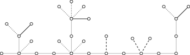
Figure 10.1: A graph $G$ with five boughs, two of which are degenerate. We draw one possible choice of free leaves. Free leaves are drawn with solid lines, bound leaves with dotted lines, and degenerate leaves with dashed lines.

Definition 10.2.

A leaf is degenerate if it belongs to a degenerate bough. For each nondegenerate bough $T$, we choose a maximal subset of leaves $\mathcal{L}_{T}\subset\mathcal{E}(T)$ with the properties that

1. no leaf in $\mathcal{L}_{T}$ is incident to the root of $T$,

2. no two leaves of $\mathcal{L}_{T}$ are adjacent.

We call the leaves in $\mathcal{L}_{T}$ free, and the remaining leaves of $\mathcal{E}(T)$ bound.

Note that, by definition, each bound leaf is adjacent to a free leaf. Thus, in a nondegenerate bough, each group of adjacent leaves contains precisely one free leaf.

Next, we introduce a total order $\preceq$ on $\mathcal{E}(G\cup G^{\prime})$, as in Section 9, which will dictate the order of summation over the labels of the bough vertices. As in Section 9, we denote by $\sigma(e)$ the immediate successor of $e$ with respect to $\preceq$ (provided that $e$ is not the last edge of $\mathcal{E}(G\cup G^{\prime})$). We impose the following conditions of $\preceq$.

1. If $e$ and $e^{\prime}$ are both bough edges and $e^{\prime}$ is the parent of $e$ then $e\prec e^{\prime}$.

2. A free leaf immediately precedes its parent: If $e$ is a free leaf then $\sigma(e)$ is the parent of $e$.

3. Nondegenerate boughs precede degenerate boughs which precede the stem: If $e$ belongs to a nondegenerate bough, $e^{\prime}$ to a degenerate bough, and $e^{\prime\prime}$ to the stem, then $e\prec e^{\prime}\prec e^{\prime\prime}$.

These properties encode the plan that children will be summed up before their parents (as in Section 9) and, additionally, in case of the free leaves, their parents will be summed up immediately after them. Furthermore, nondegenerate edges will be summed up before the degenerate ones.

It is easy to see that an order satisfying (i)–(iii) exists on $\mathcal{E}(G\cup G^{\prime})$. We choose one such order and consider it fixed in the sequel.

As in Section 9, we parametrize a general lumping $\Gamma\in\mathscr{G}(G\cup G^{\prime})$ with a pair $(\widetilde{\Gamma},A)\in\mathscr{G}_{u,u^{\prime}}\times\mathscr{A}(G\cup G^{\prime})$, where $u$ and $u^{\prime}$ denote the number of edges in $\mathcal{E}(\mathcal{S}(G))$ and $\mathcal{E}(\mathcal{S}(G^{\prime}))$ respectively. See Definitions 9.2 and 9.3, as well as Lemma 9.4.

10.3 Sum over nondegenerate bough labels

We start by summing over the bough labels $\bm{\mathrm{x}}_{B}$ in (9.11), which we recall here for convenience:

$$E_{\mathcal{G}\cup\mathcal{G}^{\prime}}\;\leqslant\;\sum_{\widetilde{\Gamma}\in\mathscr{G}_{u,u^{\prime}}}\;\sum_{\bm{\mathrm{x}}_{S}\,:\,\Gamma(\bm{\mathrm{x}}_{S})=\widetilde{\Gamma}}Q(\bm{\mathrm{x}}_{S})\\ \times\sum_{A}\;\sum_{\bm{\mathrm{x}}_{B}}\Biggl{[}{\prod_{e\in\mathcal{E}_{B}}\bm{\mathrm{1}}\bigl{(}{\varrho_{\bm{\mathrm{x}}}(e)=\varrho_{\bm{\mathrm{x}}}(A_{e})}\bigr{)}}\Biggr{]}\prod_{\gamma\in\Gamma(\widetilde{\Gamma},A)}\biggl{\lvert}\mathbb{E}\prod_{e\in\gamma}P_{\tau(e)}\bigl{(}{\widehat{H}_{x_{a(e)}x_{b(e)}},\widehat{H}_{x_{b(e)}x_{a(e)}}}\bigr{)}\biggr{\rvert}\,.$$ (10.1)

In this subsection we sum over the vertex labels of nondegenerate boughs.

Definition 10.3.

Denote by $e_{0}$ the first (with respect to $\preceq$) edge of $\mathcal{E}(G\cup G^{\prime})$, by $e_{d}$ the first edge of the degenerate boughs, and by $e_{s}$ the first stem edge. If there are no degenerate boughs, set $e_{d}=e_{s}$.

Note that, by definition of $\preceq$, we have $e_{0}\preceq e_{d}\preceq e_{s}$ (where equality is possible).

As in Section 9, we sum over the bough labels successively using a running edge $\bar{e}$. We start with $\bar{e}=e_{0}$, the first edge in $\mathcal{E}(G\cup G^{\prime})$, and after each step redefine $\bar{e}$ to be $\sigma(\bar{e})$; we stop when $\bar{e}=e_{d}$. We use the abbreviations $B^{(\bar{e})}$, $\bm{\mathrm{x}}^{(\bar{e})}$, and $A^{(\bar{e})}$ from Section 9; see (9.16) and (9.17).

We shall need one additional bough tag, $(b,6)$. Its associated polynomial is defined by (we also recall the definition of $P_{(b,5)}$ from Section 9)

$$P_{(b,5)}(\widehat{H}_{xy},\widehat{H}_{yx})\;=\;2M^{2\delta}\sigma^{2}_{xy}\,,\qquad P_{(b,6)}(\widehat{H}_{xy},\widehat{H}_{yx})\;\mathrel{\mathop{:}}=\;2M^{-1+\mu+5\delta}\sigma^{2}_{xy}\,.$$ (10.2)

As in Section 9, we consider first the special case that all nonleaf bough edges are large, i.e. have tag $(b,0)$.

We recall that a bough edge $e\in\mathcal{E}_{B}$ is lonely whenever $A_{e}=e$ and there is no $e^{\prime}\prec e$ satisfying $A_{e^{\prime}}=e$. This is equivalent to saying that $e$ is the only edge in its lump of $\Gamma(\widetilde{\Gamma},A)$. We define a new tagging $\widetilde{\tau}$ through

$$\widetilde{\tau}(e)\;\mathrel{\mathop{:}}=\;\begin{cases}\tau(e)&\text{if $e$ is not a bough leaf}\\ (b,6)&\text{if $e$ is a lonely bough leaf}\\ (b,5)&\text{if $e$ is a nonlonely leaf}\,.\end{cases}$$

Note that this tagging $\widetilde{\tau}$ is different from the one used in Section 9. The role of the new tag $(b,6)$ is to encode the gain from a lonely leaf, similarly to (9.12), but the estimate will be somewhat weaker.

Using Proposition 6.6 (ii) and Lemma 5.3 it is now easy to see that in (10.1) we have the bound

$$\prod_{\gamma\in\Gamma(\widetilde{\Gamma},A)}\biggl{\lvert}\mathbb{E}\prod_{e\in\gamma}P_{\tau(e)}\bigl{(}{\widehat{H}_{x_{a(e)}x_{b(e)}},\widehat{H}_{x_{b(e)}x_{a(e)}}}\bigr{)}\biggr{\rvert}\;\leqslant\;\prod_{\gamma\in\Gamma(\widetilde{\Gamma},A)}\mathbb{E}\prod_{e\in\gamma}\Bigl{\lvert}P_{\widetilde{\tau}(e)}\bigl{(}{\widehat{H}_{x_{a(e)}x_{b(e)}},\widehat{H}_{x_{b(e)}x_{a(e)}}}\bigr{)}\Bigr{\rvert}\,.$$ (10.3)

At this point the definition (10.2) deserves a comment. It seems that the bound (10.3) with the definition of $P_{(b,6)}$ is wasteful; indeed, (10.3) would be correct even if on the right-hand side of the second equation of (10.2) we replaced $M^{-1+\mu+5\delta}$ with $M^{-1+2\delta}$. This difference is of no consequence for our estimates, however, as the critical contribution to (10.3) comes not from lonely leaves, but from leaves lumped with other leaves, as explained around (9.7) and (9.12). Hence the wasteful additional factor $M^{\mu+3\delta}$ is of no consequence. The factor $M^{-1+\mu+5\delta}$ is designed with the transferring of entropy factors $M^{\mu}$ in mind, as explained in Section 10.1. This turns out to be the correct choice for the algorithm contained in Proposition 10.5 below.

Next, we introduce a generalization of the notion of loneliness that is relative to the running edge.

Definition 10.4.

Let $\bar{e}\in\mathcal{E}_{B}$ be the running edge. We say that an edge $e\in\mathcal{E}_{B}$ is lonely in $A^{(\bar{e})}$ whenever $A_{e}=e$ and there is no $e^{\prime}\prec e$ satisfying $e^{\prime}\in B^{(\bar{e})}$ and $A_{e^{\prime}}=e$.

Clearly, $e$ is lonely if and only if $e$ is lonely in $A^{(e_{0})}=A$ (since $e_{0}$ is the first edge of $\mathcal{E}_{B}$).

In order to get an adequate estimate from the successive summation over the nondegenerate bough labels, we shall need that, at each step indexed by $\bar{e}$ of the recursion, every leaf that is lonely in $A^{(\bar{e})}$ is small in the sense that it has tag $(b,6)$. Thus, we shall have to dynamically modify the bough tagging. To this end, let

$$\tau^{(\bar{e})}\;=\;\bigl{(}{\tau^{(\bar{e})}(e)\,:\,e\succeq\bar{e}}\bigr{)}$$

denote a tagging on the set of edges $\bigl{\{}{e\in\mathcal{E}(G\cup G^{\prime})\,:\,e\succeq\bar{e}}\bigr{\}}$. The tag $\tau^{(\bar{e})}(e)$ will indicate the actual weight of the edge $e$ after summing out all edges before $\bar{e}$, i.e. it will take into account the reallocation of the weights.

In analogy to (9.18), we define

$$R^{(\bar{e})}(\tau^{(\bar{e})})\;\mathrel{\mathop{:}}=\;\sum_{\bm{\mathrm{x}}^{(\bar{e})}}\Biggl{[}{\;\prod_{e\in B^{(\bar{e})}}\bm{\mathrm{1}}\bigl{(}{\varrho_{\bm{\mathrm{x}}}(e)=\varrho_{\bm{\mathrm{x}}}(A_{e})}\bigr{)}}\Biggr{]}\prod_{\gamma\in\Gamma(\widetilde{\Gamma},A^{(\bar{e})})}\mathbb{E}\prod_{e\in\gamma}\bigl{\lvert}P_{\tau^{(\bar{e})}(e)}\bigl{(}{\widehat{H}_{x_{a(e)}x_{b(e)}},\widehat{H}_{x_{b(e)}x_{a(e)}}}\bigr{)}\bigr{\rvert}\,.$$ (10.4)

If $\bar{e}$ is not a bough edge, we set $R^{(\bar{e})}(\tau^{(\bar{e})})\mathrel{\mathop{:}}=1$.

We define the initial tagging through $\tau^{(e_{0})}\mathrel{\mathop{:}}=\widetilde{\tau}$. Now (10.3) immediately implies that in (10.1) we may bound

$$\sum_{\bm{\mathrm{x}}_{B}}\Biggl{[}{\prod_{e\in\mathcal{E}_{B}}\bm{\mathrm{1}}\bigl{(}{\varrho_{\bm{\mathrm{x}}}(e)=\varrho_{\bm{\mathrm{x}}}(A_{e})}\bigr{)}}\Biggr{]}\prod_{\gamma\in\Gamma(\widetilde{\Gamma},A)}\biggl{\lvert}\mathbb{E}\prod_{e\in\gamma}P_{\tau(e)}\bigl{(}{\widehat{H}_{x_{a(e)}x_{b(e)}},\widehat{H}_{x_{b(e)}x_{a(e)}}}\bigr{)}\biggr{\rvert}\;\leqslant\;R^{(e_{0})}(\tau^{(e_{0})})\,.$$ (10.5)

We shall construct a sequence of taggings $\tau^{(e_{0})},\tau^{(\sigma(e_{0}))},\tau^{(\sigma^{2}(e_{0}))},\dots$ that satisfies the following property at each step $\bar{e}$.

• If $e\in B^{(\bar{e})}$ is a leaf then $\tau^{(\bar{e})}(e)\in\{(b,5),(b,6)\}$. If in addition $e$ is lonely in $A^{(\bar{e})}$ then $\tau^{(\bar{e})}(e)=(b,6)$.

To start the iteration in $\bar{e}$, we note that by definition of $\widetilde{\tau}$, the initial property $(\mathrm{L}_{e_{0}})$ holds.

The next proposition allows us to sum out a nondegenerate bough edge $\bar{e}$, i.e. perform one step of the iteration. Before stating it, we give its main idea. If $\bar{e}$ is a nonleaf edge or a bound leaf, we sum over the label $x_{b(\bar{e})}$ in (10.4). The resulting bound is given by a number $\xi$ resulting from the summation over $x_{b(\bar{e})}$ multiplied with $R^{(\sigma(\bar{e}))}$. We use the fact that, by $(\mathrm{L}_{\bar{e}})$, a lonely leaf in $A^{(\bar{e})}$ is small in the sense that it carries a factor $M^{-1+\mu+5\delta}$. In order to be able to iterate this procedure, we need that $(\mathrm{L}_{\sigma(\bar{e})})$ be satisfied. This is not true if $A_{\bar{e}}$ is a bough leaf that is lonely in $A^{(\sigma(\bar{e}))}$. We remedy this by introducing a factor $1=M^{1-\mu-3\delta}\,M^{-1+\mu+3\delta}$, and absorbing the first term into $\xi$ and the second into $R^{(\sigma(\bar{e}))}$. This will be implemented by changing the tag $\tau^{(\bar{e})}(A_{\bar{e}})=(b,5)$ to $\tau^{(\sigma(\bar{e}))}(A_{\bar{e}})=(b,6)$.

In the case that $\bar{e}$ is a free leaf, we have to extract a factor $M^{-1+\mu+5\delta}$ from the summation over $x_{b(\bar{e})}$. This is relatively easy if $\bar{e}$ is lonely in $A^{(\bar{e})}$; otherwise we need to distinguish further cases. The most involved case, in particular, occurs when $A_{\bar{e}}\succ\bar{e}$ and $A_{\bar{e}}$ is a leaf that is lonely in $A^{(\sigma(\bar{e}))}$ (i.e. the lump of $\bar{e}$ in $A^{(\bar{e})}$ consists only of two elements, $\bar{e}$ and $A_{\bar{e}}$). In this case we need to change the tag of $A_{\bar{e}}$ in $\tau^{(\sigma(\bar{e}))}$ to $(b,6)$, as described above. The resulting factor $\xi$ is of order $M^{-1+2\delta}M^{1-\mu-3\delta}$, which is much too large (here $M^{-1+2\delta}$ comes from (9.12) exactly as in Lemma 9.6, while $M^{1-\mu-3\delta}$ comes from the reallocation of this factor into $\xi$ explained in the previous paragraph). We remedy this by exploiting the fact that the label of $a(\bar{e})$ is also fixed by the lumping. Thus, we perform two summations in one step: over $x_{b(\bar{e})}$ as well as over $x_{a(\bar{e})}=x_{b(\sigma(\bar{e}))}$. In other words, we sum out both $\bar{e}$ and its successor $\sigma(\bar{e})$ at the same time. Together these summations yield a factor of order $M^{-1+\mu+5\delta}$, which is small enough.

We shall need to distinguish several different cases, which leads to a somewhat lengthy statement of the iteration step. The reason is that the worst-case estimates, which arise in the case $A_{\bar{e}}=\bar{e}$ (or, if $\bar{e}$ is a free leaf, in the cases where we do not have $A_{\bar{e}}\notin\{\bar{e},\sigma(\bar{e})\}$ and $A_{\sigma(\bar{e})}\succ\sigma(\bar{e})$) are not good enough for the following step of summing over lumpings (done in Subsection 10.5). In the case $A_{\bar{e}}=\bar{e}$, we shall need to compensate the poor estimate by the smallness of the entropy factor associated with the summation over $A_{\bar{e}}$ (namely $1$). In the case $A_{\bar{e}}\succ\bar{e}$, this same entropy factor is much larger (of the order $M^{\mu}$), but the estimate on $\xi$ is sufficiently strong to compensate for this. The following Proposition collects the estimates for the various cases.

Proposition 10.5.

Assume that $\bar{e}\in\mathcal{E}_{B}$ is a nondegenerate bough edge and that $(\mathrm{L}_{\bar{e}})$ holds.

1. If $\bar{e}$ is not a leaf, then there exists a tagging $\tau^{(\sigma(\bar{e}))}$ satisfying $(\mathrm{L}_{\sigma(\bar{e})})$ as well as the estimate

   $$R^{(\bar{e})}(\tau^{(\bar{e})})\;\leqslant\;\xi\,R^{(\sigma(\bar{e}))}(\tau^{(\sigma(\bar{e}))})\,,$$

   where

   $$\xi\;\mathrel{\mathop{:}}=\;\begin{cases}1&\text{if }A_{\bar{e}}=\bar{e}\\ 2M^{-1+2\delta}&\text{if }A_{\bar{e}}\succ\bar{e}\text{ and $A_{\bar{e}}$ is not a leaf}\\ 2M^{-\mu-\delta}&\text{if }A_{\bar{e}}\succ\bar{e}\text{ and $A_{\bar{e}}$ is a leaf}\,.\end{cases}$$ (10.6)

2. If $\bar{e}$ is a bound leaf, then there exists a tagging $\tau^{(\sigma(\bar{e}))}$ satisfying $(\mathrm{L}_{\sigma(\bar{e})})$ as well as the estimate

   $$R^{(\bar{e})}(\tau^{(\bar{e})})\;\leqslant\;\xi\,R^{(\sigma(\bar{e}))}(\tau^{(\sigma(\bar{e}))})\,,$$

   where

   $$\xi\;\mathrel{\mathop{:}}=\;2M^{-\mu-\delta}\,.$$ (10.7)

3. If $\bar{e}$ is a free leaf, then there exists a tagging $\tau^{(\sigma^{2}(\bar{e}))}$ satisfying $(\mathrm{L}_{\sigma^{2}(\bar{e})})$ as well as the estimate

   $$R^{(\bar{e})}(\tau^{(\bar{e})})\;\leqslant\;\xi\,R^{(\sigma^{2}(\bar{e}))}\bigl{(}{\tau^{(\sigma^{2}(\bar{e}))}}\bigr{)}\,,$$

   where

   $$\xi\;\mathrel{\mathop{:}}=\;\begin{cases}2M^{-1+\mu+5\delta}&\text{if }A_{\bar{e}}\in\{\bar{e},\sigma(\bar{e})\}\text{ and }A_{\sigma(\bar{e})}=\sigma(\bar{e})\\ 2M^{-1+4\delta}&\text{if }A_{\bar{e}}\in\{\bar{e},\sigma(\bar{e})\}\text{ and }A_{\sigma(\bar{e})}\succ\sigma(\bar{e})\\ 2M^{-1-\mu+\delta}&\text{if }A_{\bar{e}}\notin\{\bar{e},\sigma(\bar{e})\}\,.\end{cases}$$ (10.8)

The form of (10.8) is crucial for the later summation over the lumpings $A_{\bar{e}}$ and $A_{\sigma(\bar{e})}$. The entropy factor from each such summation is $O(1)$ if we have a “hard constraint” (i.e. that constrains $A_{\bar{e}}$ (or $A_{\sigma(\bar{e})}$) to one or two edges), and $M^{\mu}$ if we have no hard constraint. Thus, summing over the lumpings $A_{\bar{e}}$ and $A_{\sigma(\bar{e})}$ yields an entropy factor $M^{\mu(2-i)}$, where $i=0,1,2$ is the number of hard constraints. It is easy to see from (10.8) that $\xi M^{\mu(2-i)}$ is always bounded by $M^{-1+\mu+O(\delta)}$.

Proof of Proposition 10.5.

In order to avoid needless special cases throughout the proof, we shall always assume that $A_{\bar{e}}$ and $A_{\sigma(\bar{e})}$ are leaves, unless otherwise stated. This assumption always covers the worst case scenario.

We begin with Case (i). The cases $A_{\bar{e}}=\bar{e}$ and $A_{\bar{e}}\succ\bar{e}$, $A_{\bar{e}}$ not a leaf, are dealt with exactly as in the proof of Lemma 9.6; see (9.19) and (9.20). In both cases we set $\tau^{(\sigma(\bar{e}))}(e)\mathrel{\mathop{:}}=\tau^{\bar{e}}(e)$ for all $e\succeq\sigma(\bar{e})$.

If $A_{\bar{e}}\succ\bar{e}$ is a leaf we get from (9.20)

$$R^{(\bar{e})}(\tau^{(\bar{e})})\;\leqslant\;2M^{-1+2\delta}R^{(\sigma(\bar{e}))}(\tau^{(\bar{e})})\;=\;2M^{-\mu-\delta}M^{-1+\mu+3\delta}R^{(\sigma(\bar{e}))}(\tau^{(\bar{e})})\;\leqslant\;2M^{-\mu-\delta}R^{(\sigma(\bar{e}))}(\tau^{(\sigma(\bar{e}))})\,,$$

where $\tau^{(\sigma(\bar{e}))}$ is defined as

$$\tau^{(\sigma(\bar{e}))}(e)\;\mathrel{\mathop{:}}=\;\begin{cases}\tau^{(\bar{e})}(e)&\text{if }e\neq A_{\bar{e}}\\ (b,6)&\text{if }e=A_{\bar{e}}\,,\end{cases}$$ (10.9)

i.e. the gain of size $M^{-1+2\delta}$ from the summation over $x_{b(\bar{e})}$ is not exploited immediately in $\xi$, but a part of size $M^{-1+\mu+3\delta}$ is reallocated to the tag of $A_{\bar{e}}$. Here we used the bound

$$M^{-1+\mu+3\delta}\bigl{\lvert}P_{(b,5)}(\widehat{H}_{xy},\widehat{H}_{yx})\bigr{\rvert}\;\leqslant\;\bigl{\lvert}P_{(b,6)}(\widehat{H}_{xy},\widehat{H}_{yx})\bigr{\rvert}\,,$$

which we tacitly make use of in the rest of the proof. Note that the second line of (10.9) guarantees that $(L_{\sigma(\bar{e})})$ holds.

Next, we consider Case (ii). If $A_{\bar{e}}=\bar{e}$, i.e. $\bar{e}$ is lonely in $A^{(\bar{e})}$, then we use (2.7) and the fact that the property $(\mathrm{L}_{\bar{e}})$ implies $\tau^{(\bar{e})}(\bar{e})=(b,6)$. Hence, by (10.2), we get

$$R^{(\bar{e})}(\tau^{(\bar{e})})\;\leqslant\;2M^{-1+\mu+5\delta}R^{(\sigma(\bar{e}))}(\tau^{(\bar{e})})\;\leq\;2M^{-\mu-\delta}R^{(\sigma(\bar{e}))}(\tau^{(\sigma(\bar{e}))})\,,$$

where we set $\tau^{(\sigma(\bar{e}))}(e)\mathrel{\mathop{:}}=\tau^{(\bar{e})}(e)$ for $e\succeq\sigma(\bar{e})$. If $A_{\bar{e}}\succ\bar{e}$ we define $\tau^{(\sigma(\bar{e}))}$ through (10.9) and get, as in the proof of Case (i),

$$R^{(\bar{e})}(\tau^{(\bar{e})})\;\leqslant\;2M^{-\mu-\delta}R^{(\sigma(\bar{e}))}(\tau^{(\sigma(\bar{e}))})\,.$$

Again, one can easily check that $(L_{\sigma(\bar{e})})$ holds.

Now consider Case (iii). By property (ii) of the order $\prec$, we know that $\sigma(\bar{e})$ is the parent of $\bar{e}$, i.e. $b(\sigma(\bar{e}))=a(\bar{e})$. Note that in this case we sum out the two edges $\bar{e}$ and $\sigma(\bar{e})$ in one step.

Consider first the case $A_{\bar{e}}=\bar{e}$ and $A_{\sigma(\bar{e})}=\sigma(\bar{e})$. Then $\tau^{(\bar{e})}(\bar{e})=(b,6)$ and $\tau^{(\bar{e})}(\sigma(\bar{e}))=(b,0)$ by assumption. Therefore summing over $x_{b(\bar{e})}$ and $x_{a(\bar{e})}=x_{b(\sigma(\bar{e}))}$ using (10.2) and (2.7) yields

$$R^{(\bar{e})}(\tau^{(\bar{e})})\;\leqslant\;2M^{-1+\mu+5\delta}R^{(\sigma^{2}(\bar{e}))}\bigl{(}{\tau^{(\sigma^{2}(\bar{e}))}}\bigr{)}\,,$$

where $\tau^{(\sigma^{2}(\bar{e}))}(e)\mathrel{\mathop{:}}=\tau^{(\bar{e})}(e)$. In the case $A_{\bar{e}}=A_{\sigma(\bar{e})}=\sigma(\bar{e})$ we have that $\tau^{(\bar{e})}(\bar{e})$ is either $(b,5)$ or $(b,6)$, and $\tau^{(\bar{e})}(\sigma(\bar{e}))=(b,0)$. Thus (10.2) and (2.7) imply

$$R^{(\bar{e})}(\tau^{(\bar{e})})\;\leqslant\;2M^{-1+2\delta}R^{(\sigma^{2}(\bar{e}))}\bigl{(}{\tau^{(\sigma^{2}(\bar{e}))}}\bigr{)}\,,$$

where $\tau^{(\sigma^{2}(\bar{e}))}(e)\mathrel{\mathop{:}}=\tau^{(\bar{e})}(e)$. It is easy to see that $(\mathrm{L}_{\sigma^{2}(\bar{e})})$ holds. We have covered the first line of (10.8).

Next, consider the case $A_{\bar{e}}=\bar{e}$ and $A_{\sigma(\bar{e})}\succ\sigma(\bar{e})$. Then, using that $\bar{e}$ is lonely in $A^{\bar{e}}$ (and hence carries a tag $(b,6)$ by $(\mathrm{L}_{\bar{e}})$) and that $x_{b(\sigma(\bar{e}))}$ is fixed, we get the bound

$$R^{(\bar{e})}(\tau^{(\bar{e})})\;\leqslant\;2M^{-1+\mu+5\delta}M^{-1+2\delta}R^{(\sigma^{2}(\bar{e}))}(\tau^{(\bar{e})})\;=\;2M^{-1+4\delta}M^{-1+\mu+3\delta}R^{(\sigma^{2}(\bar{e}))}(\tau^{(\bar{e})})\\ \leqslant\;2M^{-1+4\delta}R^{(\sigma^{2}(\bar{e}))}(\tau^{(\sigma^{2}(\bar{e}))})\,,$$

where we set

$$\tau^{(\sigma^{2}(\bar{e}))}(e)\;\mathrel{\mathop{:}}=\;\begin{cases}\tau^{(\bar{e})}(e)&\text{if }e\neq A_{\sigma(\bar{e})}\\ (b,6)&\text{if }e=A_{\sigma(\bar{e})}\,;\end{cases}$$ (10.10)

thus, $(\mathrm{L}_{\sigma^{2}(\bar{e})})$ holds. Similarly, if $A_{\bar{e}}=\sigma(\bar{e})$ and $A_{\sigma(\bar{e})}\succ\sigma(\bar{e})$ then $x_{b(\bar{e})}$ and $x_{b(\sigma(\bar{e}))}$ are fixed by $A_{\bar{e}}$ and we get

$$R^{(\bar{e})}(\tau^{(\bar{e})})\;\leqslant\;2M^{-1+2\delta}M^{-1+2\delta}R^{(\sigma^{2}(\bar{e}))}(\tau^{(\bar{e})})\;=\;2M^{-1-\mu+\delta}M^{-1+\mu+3\delta}R^{(\sigma^{2}(\bar{e}))}(\tau^{(\bar{e})})\\ \leqslant\;2M^{-1-\mu+\delta}R^{(\sigma^{2}(\bar{e}))}(\tau^{(\sigma^{2}(\bar{e}))})\,,$$

where we define $\tau^{(\sigma^{2}(\bar{e}))}$ through (10.10). This covers the second line of (10.8).

We now turn to the last line of (10.8). Consider the case $A_{\bar{e}}\notin\{\bar{e},\sigma(\bar{e})\}$ and $A_{\sigma(\bar{e})}=\sigma(\bar{e})$. Thus $x_{b(\bar{e})}$ and $x_{b(\sigma(\bar{e}))}$ are fixed by $A_{\bar{e}}$, and we have

$$R^{(\bar{e})}(\tau^{(\bar{e})})\;\leqslant\;2M^{-1+2\delta}M^{-1+2\delta}R^{(\sigma^{2}(\bar{e}))}(\tau^{(\bar{e})})\;=\;2M^{-1-\mu+\delta}M^{-1+\mu+3\delta}R^{(\sigma^{2}(\bar{e}))}(\tau^{(\bar{e})})\\ \leqslant\;2M^{-1-\mu+\delta}R^{(\sigma^{2}(\bar{e}))}(\tau^{(\sigma^{2}(\bar{e}))})\,,$$

where we set

$$\tau^{(\sigma^{2}(\bar{e}))}(e)\;\mathrel{\mathop{:}}=\;\begin{cases}\tau^{(\bar{e})}(e)&\text{if }e\neq A_{\bar{e}}\\ (b,6)&\text{if }e=A_{\bar{e}}\,,\end{cases}$$

passing part of the total gain from the double summation to $A_{\bar{e}}$. In particular, $(\mathrm{L}_{\sigma^{2}(\bar{e})})$ holds.

Next, consider the case $A_{\bar{e}}\notin\{\bar{e},\sigma(\bar{e})\}$ and $A_{\sigma(\bar{e})}\succ\sigma(\bar{e})$. Assume first that $A_{\bar{e}}$ and $A_{\sigma(\bar{e})}$ are not both bough leaves that are lonely in $A^{(\sigma^{2}(\bar{e}))}$. Then we get, using again that $x_{b(\bar{e})}$ and $x_{b(\sigma(\bar{e}))}$ are fixed by $A_{\bar{e}}$, that

$$R^{(\bar{e})}(\tau^{(\bar{e})})\;\leqslant\;2M^{-1+2\delta}M^{-1+2\delta}R^{(\sigma^{2}(\bar{e}))}(\tau^{(\bar{e})})\;=\;2M^{-1-\mu+\delta}M^{-1+\mu+3\delta}R^{(\sigma^{2}(\bar{e}))}(\tau^{(\bar{e})})\\ \leqslant\;2M^{-1-\mu+\delta}R^{(\sigma^{2}(\bar{e}))}(\tau^{(\sigma^{2}(\bar{e}))})\,,$$

where we set

$$\tau^{(\sigma^{2}(\bar{e}))}(e)\;\mathrel{\mathop{:}}=\;\begin{cases}(b,6)&\text{if }e\in\{{A_{\bar{e}},A_{\sigma(\bar{e})}}\}\text{ is a leaf lonely in }A^{(\sigma^{2}(\bar{e}))}\\ \tau^{(\bar{e})}(e)&\text{otherwise}\,.\end{cases}$$

Here we used that, in order for $(\mathrm{L}_{\sigma^{2}(\bar{e})})$ to hold, we need at most one of the bough edges $A_{\bar{e}}$ and $A_{\sigma(\bar{e})}$ to receive the tag $(b,6)$ in $\tau^{(\sigma^{2}(\bar{e}))}$.

Finally, we consider the case where both $A_{\bar{e}}=\mathrel{\mathop{:}}e^{\prime}\notin\{\bar{e},\sigma(\bar{e})\}$ and $A_{\sigma(\bar{e})}=\mathrel{\mathop{:}}e^{\prime\prime}\succ\sigma(\bar{e})$ are bough leaves that are lonely in $A^{(\sigma^{2}(\bar{e}))}$. Although our goal is to sum out only the edges $\bar{e}$ and $\sigma(\bar{e})$, it will prove necessary to first sum out all four edges $\bar{e},\sigma(\bar{e}),e^{\prime},e^{\prime\prime}$ in order to get a sufficiently strong reduction of the entropy factor. Having done this, we put back the sum over the end-labels of $e^{\prime}$ and $e^{\prime\prime}$ (thus undoing their “striking” out of the graph that resulted from summing them out) to get the needed factor $R^{(\sigma^{2}(\bar{e}))}(\tau^{(\bar{e})})$.

Thus, we sum over all the labels of the four vertices $b(\bar{e}),b(\sigma(\bar{e})),b(e^{\prime})$, and $b(e^{\prime\prime})$ in the expression for $R^{(\bar{e})}(\tau^{(\bar{e})})$; we fix all other labels. Now it is easy to see that the label $x_{b(e^{\prime})}$ uniquely determines the other three labels, so the total entropy factor for these summations is $M$. Hence summing over the above four labels in the expression for $R^{(\bar{e})}(\tau^{(\bar{e})})$ yields the bound

$$R^{(\bar{e})}(\tau^{(\bar{e})})\;\leqslant\;(2M^{2\delta})^{3}M^{-3}\,\widetilde{R}\,,$$

where $\widetilde{R}$ is the expression obtained from $R^{(\bar{e})}(\tau^{(\bar{e})})$ by summing out the edges $\bar{e},\sigma(\bar{e}),e^{\prime},e^{\prime\prime}$. (In the estimate we used the worst case scenario, in which the edges $\bar{e},e^{\prime},e^{\prime\prime}$ are of type $(b,5)$ and the edge $\sigma(\bar{e})$ of type $(b,0)$.) Next, it is easy to see that summing out the two edges $e^{\prime}$ and $e^{\prime\prime}$ in the expression for $R^{(\sigma^{2}(\bar{e}))}(\tau^{(\bar{e})})$ gives the equality

$$R^{(\sigma^{2}(\bar{e}))}(\tau^{(\bar{e})})\;=\;(2M^{2\delta})^{2}\widetilde{R}\,$$

since at the moment when $\bar{e}$ is summed out, both $e^{\prime}$ and $e^{\prime\prime}$ are nonlonely bough leaves, thus $\tau^{(\bar{e})}(e^{\prime})=\tau^{(\bar{e})}(e^{\prime\prime})=(b,5)$. Thus we find

$$R^{(\bar{e})}(\tau^{(\bar{e})})\;\leqslant\;2M^{-3+2\delta}R^{(\sigma^{2}(\bar{e}))}(\tau^{(\bar{e})})\;=\;2M^{-1-2\mu-4\delta}\bigl{(}{M^{-1+\mu+3\delta}}\bigr{)}^{2}R^{(\sigma^{2}(\bar{e}))}(\tau^{(\bar{e})})\\ \leqslant\;2M^{-1-2\mu-4\delta}R^{(\sigma^{2}(\bar{e}))}(\tau^{(\sigma^{2}(\bar{e}))})\,,$$

where we set

$$\tau^{(\sigma^{2}(\bar{e}))}(e)\;\mathrel{\mathop{:}}=\;\begin{cases}(b,6)&\text{if }e\in\{{A_{\bar{e}},A_{\sigma(\bar{e})}}\}\\ \tau^{(\bar{e})}(e)&\text{otherwise}\,.\end{cases}$$

The factor $\bigl{(}{M^{-1+\mu+3\delta}}\bigr{)}^{2}$ is absorbed into $R^{(\bar{e})}(\tau^{(\bar{e})})$ to get $R^{(\bar{e})}(\tau^{(\sigma^{2}(\bar{e}))})$ and at the same time ensure that $(\mathrm{L}_{\sigma^{2}(\bar{e})})$ is satisfied. This covers the third line of (10.8), and hence concludes the proof. ∎

10.4 Sum over degenerate bough labels

In this subsection we sum over all labels associated with degenerate bough edges, having already summed out the nondegenerate boughs in the previous section. We estimate $R^{(e_{d})}(\tau^{(e_{d})})$, where $e_{d}$ is the first degenerate bough edge of $\mathcal{E}_{B}$, and $\tau^{(e_{d})}$ is a tagging satisfying $(\mathrm{L}_{e_{d}})$. Our strategy is very similar to Subsection 9.3. For $e\in B^{(e_{d})}$ (i.e. $e_{d}\preceq e\prec e_{s}$) we define the inverse $A^{-1}_{e}$ by restricting Definition 9.5 to $B^{(e_{d})}$. In other words, we define $A_{e}^{-1}\mathrel{\mathop{:}}=e^{\prime}$ if there exists a (necessarily unique) $e^{\prime}$ satisfying $e_{d}\preceq e^{\prime}\prec e$ and $A_{e^{\prime}}=e$. Otherwise we set $A_{e}^{-1}\mathrel{\mathop{:}}=e$.

By the assumption $(\mathrm{L}_{e_{d}})$, every leaf $e\in B^{(e_{d})}$ that is lonely in $A^{(e_{d})}$ has tag $\tau^{(e_{d})}(e)=(b,6)$. Therefore we may reproduce the proof of (9.22) verbatim to get, for a fixed ${\bm{\mathrm{x}}}_{S}$,

$$R^{(e_{d})}(\tau^{(e_{d})})\;\leqslant\;f(A)\,\prod_{\gamma\in\widetilde{\Gamma}}\mathbb{E}\prod_{e\in\gamma}\Bigl{\lvert}P_{\tau(e)}\bigl{(}{\widehat{H}_{x_{a(e)}x_{b(e)}},\widehat{H}_{x_{b(e)}x_{a(e)}}}\bigr{)}\Bigr{\rvert}\,,$$ (10.11)

where

$$f(A)\;\mathrel{\mathop{:}}=\;\prod_{e\in B^{(e_{d})}\text{ leaf}}\biggl{(}{\frac{2M^{2\delta}}{M}+\bm{\mathrm{1}}\bigl{(}{e=A_{e}}\bigr{)}\,2M^{-1+\mu+5\delta}+\bm{\mathrm{1}}\bigl{(}{A^{-1}_{e}\prec e=A_{e}}\bigr{)}\,2M^{2\delta}}\biggr{)}\,.$$ (10.12)

Note that, unlike in (9.22), the product in (10.12) ranges only over leaves, since degenerate boughs consist only of leaves.

We may now put the estimate on both nondegenerate and degenerate boughs together. From (10.5), Proposition 10.5, and (10.11) we get

$$\sum_{\bm{\mathrm{x}}_{B}}\Biggl{[}{\prod_{e\in\mathcal{E}_{B}}\bm{\mathrm{1}}\bigl{(}{\varrho_{\bm{\mathrm{x}}}(e)=\varrho_{\bm{\mathrm{x}}}(A_{e})}\bigr{)}}\Biggr{]}\prod_{\gamma\in\Gamma(\widetilde{\Gamma},A)}\biggl{\lvert}\mathbb{E}\prod_{e\in\gamma}P_{\tau(e)}\bigl{(}{\widehat{H}_{x_{a(e)}x_{b(e)}},\widehat{H}_{x_{b(e)}x_{a(e)}}}\bigr{)}\biggr{\rvert}\\ \leqslant\;F(A)\,\prod_{\gamma\in\widetilde{\Gamma}}\mathbb{E}\prod_{e\in\gamma}\Bigl{\lvert}P_{\tau(e)}\bigl{(}{\widehat{H}_{x_{a(e)}x_{b(e)}},\widehat{H}_{x_{b(e)}x_{a(e)}}}\bigr{)}\Bigr{\rvert}\,,$$ (10.13)

where

$$F(A)\;\mathrel{\mathop{:}}=\;\Biggl{[}{\;\prod_{e\in\mathcal{E}_{B}\text{ nonleaf}}\Bigl{(}{\bm{\mathrm{1}}(A_{e}=e)+2M^{-1+2\delta}+\bm{\mathrm{1}}\bigl{(}{A_{e}\succ e\text{ is a leaf}\,}\bigr{)}2M^{-\mu-\delta}}\Bigr{)}}\Biggr{]}\Biggl{[}{\;\prod_{e\in\mathcal{E}_{B}\text{ bound leaf}}2M^{-\mu-\delta}}\Biggr{]}\\ \times\prod_{e\in\mathcal{E}_{B}\text{ free leaf}}\biggl{[}\bm{\mathrm{1}}\bigl{(}{A_{e}\in\{e,\sigma(e)\}}\bigr{)}\bm{\mathrm{1}}\bigl{(}{A_{\sigma(e)}=\sigma(e)}\bigr{)}\,2M^{-1+\mu+5\delta}+\bm{\mathrm{1}}\bigl{(}{A_{e}\in\{e,\sigma(e)\}}\bigr{)}\,2M^{-1+4\delta}+2M^{-1-\mu+\delta}\biggr{]}\\ \times\prod_{e\in\mathcal{E}_{B}\text{ degenerate leaf}}\Bigl{[}{2M^{-1+2\delta}+\bm{\mathrm{1}}\bigl{(}{e=A_{e}}\bigr{)}\,2M^{-1+\mu+5\delta}+\bm{\mathrm{1}}\bigl{(}{A^{-1}_{e}\prec e=A_{e}}\bigr{)}\,2M^{2\delta}}\Bigr{]}\,.$$ (10.14)

As was advertised before the proof of Proposition 10.5, this estimate is designed to counterbalance the various smallness factors and the entropy factors for the lumping summation. For instance, in the second line, the prefactor is $M^{-1+(i-1)\mu+O(\delta)}$ where $i=0,1,2$ is the number of hard constraints, so after summation over the lumpings, each summand will be of the same order $M^{-1+\mu+5\delta}$. The same balance can be seen among the first two summands in the last line, while the last summand will be treated similarly to how the second factor in (9.23) was evaluated in Subsection 9.4. Finally, in the product over the nonleaves in the first line, only a weaker bound is available if $A_{e}\succ e$ is a leaf. But this bound is strong enough to guarantee that, even after summation over $A$, the total contribution of the nonleaves is $C^{L}$ instead of $C^{M^{\mu}}$, where $L$ is the number of leaves (see (10.18)). Since some (small, at worst $O(M^{-\delta})$) gain is available for each leaf, a factor $C^{L}$ is affordable.

10.5 General taggings and sum over bough lumpings

So far we assumed that all nonleaf bough edges had tag $(b,0)$ and all bough leaves tag $(b,1)$. As in Subsection 9.3, we split the tagging into a bough and stem tagging, $\tau=(\tau_{B},\tau_{S})$, and define

$$F(A,\tau_{B})\;\mathrel{\mathop{:}}=\;F(A)\prod_{e\in\mathcal{E}_{B}\text{ nonleaf}}\bigl{(}{M^{2\delta-1}}\bigr{)}^{\bm{\mathrm{1}}(\tau_{B}(e)\neq(b,0))}\,.$$ (10.15)

Then (10.13) for arbitrary $\tau$ holds if $F(A)$ on the right-hand side is replaced by $F(A,\tau_{B})$.

Now we sum over all bough lumpings $A\in\mathscr{A}(G\cup G^{\prime})$. We start by summing over $A_{e}$ in (10.14) for all degenerate edges $e$. Now we proceed as in Subsection 9.4. In fact, we perform the summation of Subsection 9.4 over $A$ only on the second factor of (9.23), as the (trivial) nonleaf edges are treated separately. Moreover, the additional summand in each nonleaf factor $\bm{\mathrm{1}}\bigl{(}{e=A_{e}}\bigr{)}\,2M^{-1+\mu+5\delta}$ is trivially accounted for. Thus we get

$$\sum_{A^{(e_{d})}}\;\prod_{e\in\mathcal{E}_{B}\text{ degenerate leaf}}\Bigl{[}{2M^{-1+2\delta}+\bm{\mathrm{1}}\bigl{(}{e=A_{e}}\bigr{)}\,2M^{-1+\mu+5\delta}+\bm{\mathrm{1}}\bigl{(}{A^{-1}_{e}\prec e=A_{e}}\bigr{)}\,2M^{2\delta}}\Bigr{]}\\ \leqslant\;\Bigl{(}{CM^{-1+\mu+7\delta}}\Bigr{)}^{L^{(d)}/2}\,,$$ (10.16)

where $L^{(d)}\equiv L^{(d)}(G\cup G^{\prime})$ is the number of degenerate leaves in $G\cup G^{\prime}$. From (10.1), (10.13) with an arbitrary tagging $\tau_{B}$, and (10.15) we therefore get

$$E_{\mathcal{G}\cup\mathcal{G}^{\prime}}\;\leqslant\;\Biggl{[}{\;\prod_{e\in\mathcal{E}_{B}\text{ nonleaf}}\Bigl{(}{1+2M^{-1+\mu+2\delta}+2LM^{-\mu-\delta}}\Bigr{)}\bigl{(}{M^{-1+2\delta}}\bigr{)}^{\bm{\mathrm{1}}(\tau_{B}(e)\neq(b,0))}}\Biggr{]}\Biggl{[}{\;\prod_{e\in\mathcal{E}_{B}\text{ bound leaf}}2M^{-\delta}}\Biggr{]}\\ \times\Biggl{[}{\;\prod_{e\in\mathcal{E}_{B}\text{ free leaf}}CM^{-1+\mu+5\delta}}\Biggr{]}\Bigl{(}{CM^{-1+\mu+7\delta}}\Bigr{)}^{L^{(d)}/2}\\ \times\sum_{\widetilde{\Gamma}\in\mathscr{G}_{u,u^{\prime}}}\sum_{\bm{\mathrm{x}}_{S}\,:\,\Gamma(\bm{\mathrm{x}}_{S})=\widetilde{\Gamma}}Q(\bm{\mathrm{x}}_{S})\prod_{\gamma\in\widetilde{\Gamma}}\mathbb{E}\prod_{e\in\gamma}\Bigl{\lvert}P_{\tau(e)}\bigl{(}{\widehat{H}_{x_{a(e)}x_{b(e)}},\widehat{H}_{x_{b(e)}x_{a(e)}}}\bigr{)}\Bigr{\rvert}\,,$$ (10.17)

where $L$ is the total number of bough leaves in $G\cup G^{\prime}$. Recalling that the number of edges of $G\cup G^{\prime}$ is bounded by $M^{\mu}$, we find

$$\prod_{e\in\mathcal{E}_{B}\text{ nonleaf}}\Bigl{(}{1+2M^{-1+\mu+2\delta}+2LM^{-\mu-\delta}}\Bigr{)}\;\leqslant\;C^{L}\,.$$ (10.18)

Recall that $L^{(d)}$ denotes the number of degenerate leaves of $G\cup G^{\prime}$. Similarly, denote by $L^{(b)}$ the number of bound leaves of $G\cup G^{\prime}$ and by $L^{(f)}$ the number of free leaves of $G\cup G^{\prime}$. We have proved the following result.

Proposition 10.6.

For any $\mathcal{G},\mathcal{G}^{\prime}\in\mathfrak{G}_{\sharp}$ we have

$$E_{\mathcal{G}\cup\mathcal{G}^{\prime}}\;\leqslant\;\Biggl{[}{\prod_{e\in\mathcal{E}_{B}\text{\rm nonleaf}}\bigl{(}{M^{-1+2\delta}}\bigr{)}^{\bm{\mathrm{1}}(\tau(e)\neq(b,0))}}\Biggr{]}\bigl{(}{CM^{-\delta}}\bigr{)}^{L^{(b)}}\bigl{(}{CM^{-1+\mu+5\delta}}\bigr{)}^{L^{(f)}}\bigl{(}{CM^{-1+\mu+7\delta}}\bigr{)}^{L^{(d)}/2}\\ \times\sum_{\widetilde{\Gamma}\in\mathscr{G}_{u,u^{\prime}}}\sum_{\bm{\mathrm{x}}_{S}\,:\,\Gamma(\bm{\mathrm{x}}_{S})=\widetilde{\Gamma}}Q(\bm{\mathrm{x}}_{S})\prod_{\gamma\in\widetilde{\Gamma}}\mathbb{E}\prod_{e\in\gamma}\Bigl{\lvert}P_{\tau(e)}\bigl{(}{\widehat{H}_{x_{a(e)}x_{b(e)}},\widehat{H}_{x_{b(e)}x_{a(e)}}}\bigr{)}\Bigr{\rvert}\,.$$ (10.19)

10.6 Decoupling and sum over the tagging

We now proceed as in Subsection 9.5 and prove the following result which is analogous to Lemma 9.8. In order to state it, we split

$$L^{(i)}(G\cup G^{\prime})\;=\;L^{(i)}(G)+L^{(i)}(G^{\prime})\,;$$

here $L^{(i)}(G)$ is the number of bough leaves of $G$ of type $i$, where $i$ can be $b$ (for “bound”), $f$ (for “free”), or $d$ (for “degenerate”).

Proposition 10.7.

We have

$$E_{1}\;\leqslant\;\sum_{n+n^{\prime}\leqslant M^{\mu}}\lvert\alpha_{n}(t)\alpha_{n^{\prime}}(t)\rvert\sum_{r,r^{\prime}\geqslant 0}\bigl{(}{M^{-1+2\delta}}\bigr{)}^{r+r^{\prime}}\sum_{u=0}^{n-1}\sum_{u^{\prime}=0}^{n^{\prime}-1}h_{u,u^{\prime}}\\ \times\sum_{\mathcal{G},\mathcal{G}^{\prime}\in\mathfrak{G}_{\sharp}}\Bigl{[}{\bm{\mathrm{1}}\bigl{(}{\lvert\mathcal{E}(\mathcal{S}(G))\rvert=u}\bigr{)}\bm{\mathrm{1}}\bigl{(}{\deg(\mathcal{S}(G),\tau_{S})=u+2r}\bigr{)}\bm{\mathrm{1}}\bigl{(}{2\lvert\mathcal{E}(\mathcal{B}(G))\rvert=n-u-2r}\bigr{)}}\Bigr{]}\Bigl{[}{\text{\rm primed}}\Bigr{]}\\ \times\bigl{(}{CM^{-\delta}}\bigr{)}^{L^{(b)}(G)+L^{(b)}(G^{\prime})}\bigl{(}{CM^{-1+\mu+5\delta}}\bigr{)}^{L^{(f)}(G)+L^{(f)}(G^{\prime})}\bigl{(}{CM^{-1+\mu+7\delta}}\bigr{)}^{L^{(d)}(G)/2+L^{(d)}(G^{\prime})/2}\\ \times\prod_{e\in\mathcal{E}_{B}\text{\rm nonleaf}}\bigl{(}{M^{-1+2\delta}}\bigr{)}^{\bm{\mathrm{1}}(\tau(e)\neq(b,0))}\,.$$ (10.20)

Proof.

See Appendix D. ∎

We may now sum over the bough tagging $\tau_{B}$ in (10.20) to get

$$E_{1} \;\leqslant\;\sum_{n+n^{\prime}\leqslant M^{\mu}}\lvert\alpha_{n}(t)\alpha_{n^{\prime}}(t)\rvert\sum_{r,r^{\prime}\geqslant 0}\bigl{(}{M^{-1+2\delta}}\bigr{)}^{r+r^{\prime}}\sum_{u=0}^{n-1}\sum_{u^{\prime}=0}^{n^{\prime}-1}h_{u,u^{\prime}}$$

$$\qquad\times\sum_{G,G^{\prime}\in\mathfrak{W}}\sum_{\tau_{S}}\Bigl{[}{\bm{\mathrm{1}}\bigl{(}{\lvert\mathcal{E}(\mathcal{S}(G))\rvert=u}\bigr{)}\bm{\mathrm{1}}\bigl{(}{\deg(\mathcal{S}(G),\tau_{S})=u+2r}\bigr{)}\bm{\mathrm{1}}\bigl{(}{2\lvert\mathcal{E}(\mathcal{B}(G))\rvert=n-u-2r}\bigr{)}}\Bigr{]}\Bigl{[}{\text{\rm primed}}\Bigr{]}$$

$$\qquad\times\sum_{\tau_{B}}\bigl{(}{CM^{-\delta}}\bigr{)}^{L^{(b)}(G)+L^{(b)}(G^{\prime})}\bigl{(}{CM^{-1+\mu+5\delta}}\bigr{)}^{L^{(f)}(G)+L^{(f)}(G^{\prime})}\bigl{(}{CM^{-1+\mu+7\delta}}\bigr{)}^{L^{(d)}(G)/2+L^{(d)}(G^{\prime})/2}$$

$$\qquad\times\prod_{e\in\mathcal{E}_{B}\text{\rm nonleaf}}\bigl{(}{M^{-1+2\delta}}\bigr{)}^{\bm{\mathrm{1}}(\tau(e)\neq(b,0))}$$

$$\;\leqslant\;\sum_{n+n^{\prime}\leqslant M^{\mu}}\lvert\alpha_{n}(t)\alpha_{n^{\prime}}(t)\rvert\sum_{r,r^{\prime}\geqslant 0}\bigl{(}{M^{-1+2\delta}}\bigr{)}^{r+r^{\prime}}\sum_{u=0}^{n-1}\sum_{u^{\prime}=0}^{n^{\prime}-1}h_{u,u^{\prime}}$$

$$\qquad\times\sum_{G,G^{\prime}\in\mathfrak{W}}\sum_{\tau_{S}}\Bigl{[}{\bm{\mathrm{1}}\bigl{(}{\lvert\mathcal{E}(\mathcal{S}(G))\rvert=u}\bigr{)}\bm{\mathrm{1}}\bigl{(}{\deg(\mathcal{S}(G),\tau_{S})=u+2r}\bigr{)}\bm{\mathrm{1}}\bigl{(}{2\lvert\mathcal{E}(\mathcal{B}(G))\rvert=n-u-2r}\bigr{)}}\Bigr{]}\Bigl{[}{\text{\rm primed}}\Bigr{]}$$

$$\qquad\times C\bigl{(}{CM^{-\delta}}\bigr{)}^{L^{(b)}(G)+L^{(b)}(G^{\prime})}\bigl{(}{CM^{-1+\mu+5\delta}}\bigr{)}^{L^{(f)}(G)+L^{(f)}(G^{\prime})}\bigl{(}{CM^{-1+\mu+7\delta}}\bigr{)}^{L^{(d)}(G)/2+L^{(d)}(G^{\prime})/2}\,,$$

where the second inequality follows analogously to (9.34). Next, we sum over the stem tagging $\tau_{S}$ using (9.35),

$$E_{1} \;\leqslant\;\sum_{n+n^{\prime}\leqslant M^{\mu}}\lvert\alpha_{n}(t)\alpha_{n^{\prime}}(t)\rvert\sum_{r,r^{\prime}\geqslant 0}\bigl{(}{M^{-1+\mu+2\delta}}\bigr{)}^{r+r^{\prime}}\sum_{u=0}^{n-1}\sum_{u^{\prime}=0}^{n^{\prime}-1}h_{u,u^{\prime}}$$

$$\qquad\times\sum_{G,G^{\prime}\in\mathfrak{W}}\Bigl{[}{\bm{\mathrm{1}}\bigl{(}{\lvert\mathcal{E}(\mathcal{S}(G))\rvert=u}\bigr{)}\bm{\mathrm{1}}\bigl{(}{2\lvert\mathcal{E}(\mathcal{B}(G))\rvert=n-u-2r}\bigr{)}}\Bigr{]}\Bigl{[}{\text{\rm primed}}\Bigr{]}$$

$$\qquad\times C\bigl{(}{CM^{-\delta}}\bigr{)}^{L^{(b)}(G)+L^{(b)}(G^{\prime})}\bigl{(}{CM^{-1+\mu+5\delta}}\bigr{)}^{L^{(f)}(G)+L^{(f)}(G^{\prime})}\bigl{(}{CM^{-1+\mu+7\delta}}\bigr{)}^{L^{(d)}(G)/2+L^{(d)}(G^{\prime})/2}\,$$

$$\;\leqslant\;\sum_{n+n^{\prime}\leqslant M^{\mu}}\lvert\alpha_{n}(t)\alpha_{n^{\prime}}(t)\rvert\sum_{u=0}^{n-1}\sum_{u^{\prime}=0}^{n^{\prime}-1}h_{u,u^{\prime}}$$

$$\qquad\times\Biggl{[}\sum_{r\geqslant 0}\bigl{(}{M^{-1+\mu+2\delta}}\bigr{)}^{r}\sum_{G\in\mathfrak{W}}\bm{\mathrm{1}}\bigl{(}{\lvert\mathcal{E}(\mathcal{S}(G))\rvert=u}\bigr{)}\bm{\mathrm{1}}\bigl{(}{2\lvert\mathcal{E}(\mathcal{B}(G))\rvert=n-u-2r}\bigr{)}$$

$$\qquad\times C\bigl{(}{CM^{-\delta}}\bigr{)}^{L^{(b)}(G)}\bigl{(}{CM^{-1+\mu+5\delta}}\bigr{)}^{L^{(f)}(G)}\bigl{(}{CM^{-1+\mu+7\delta}}\bigr{)}^{L^{(d)}(G)/2}\Biggr{]}\Bigl{[}{\text{\rm primed}}\Bigr{]}\,.$$ (10.21)

10.7 Sum over the bough graphs

Now we may sum over the graphs $G,G^{\prime}\in\mathfrak{W}$ in (10.21). A key ingredient is the following combinatorial estimate. Let $S_{kfb}$ be the number of nondegenerate boughs with $k$ edges, $f$ free leaves, and $b$ bound leaves. In other words, $S_{kfb}$ is the number of oriented, unlabelled, rooted trees with $k$ edges and $f+b$ leaves, such that the number of groups of adjacent leaves, excluding leaves incident to the root, is equal to $f$ (see Definition 10.2).

Lemma 10.8.

We have

$$S_{kfb}\;\leqslant\;k^{2f-2}\,2^{2f+b}\,.$$

Proof.

We construct an arbitrary nondegenerate bough corresponding to the triple $(k,f,b)$ in two steps.

1. We choose an oriented, unlabelled, rooted tree $T$ with $k-b$ edges and $f$ leaves such that no two leaves are adjacent and no leaf is incident to the root.

2. We add $b$ leaves to $T$ by requiring that each newly added leaf be either adjacent to an existing leaf or incident to the root.

Clearly, the number of possible choices for the tree $T$ in (i) is bounded by the number of oriented, unlabelled, rooted trees with $k$ edges and $f$ leaves. This was estimated in (9.39) by $k^{2f-2}$.

Next, let $\mathscr{V}$ denote the subset of vertices of $T$ consisting of the root of $T$ and of all initial vertices of the leaves of $T$. Step (ii) means that we have to add $b$ leaves to $T$ under the constraint that each newly added leaf be incident to a vertex of $\mathscr{V}$. The new leaves may be thought of as being added to a certain number, $z$, of allowed slots; each slot may receive several new leaves. The number of slots associated with a vertex $v\in\mathscr{V}$ is computed as follows. For a vertex $v$ of $T$, let $c_{v}\in\mathbb{N}$ denote the number of children of $v$ in $T$. It is easy to see that the number of slots associated with the vertex $v\in\mathscr{V}$ is equal to $c_{v}$ if $v$ is not the root and to $c_{v}+1$ if $v$ is the root. In this counting we have taken the orientation of the graph into account, i.e. existing edges are drawn in the plane, and the new edges emanate between them. Thus the number of slots associated with a leaf $e$ is equal to the number of planar “wedges” delimited by edges incident to $a(e)$, whereby the two wedges on either side of $e$ count as one; see Figure 10.2.

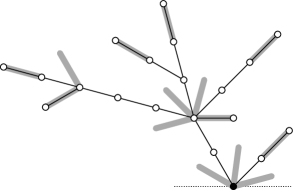
Figure 10.2: A bough with $k=19$ edges and $f=7$ free leaves. The $z=14$ slots for adding bound leaves are indicated in grey. The stem is indicated with a dotted line.

Thus, the total number of slots is $z=1+\sum_{v\in\mathscr{V}}c_{v}$. Now let us denote by $\mathscr{V}^{\prime}$ the subset of vertices of $\mathcal{V}(T)$ that are not leaf vertices (or in other words the root together with the vertices that have degree greater than one). It is easy to see that we have

$$1+\sum_{v\in\mathscr{V}^{\prime}}(c_{v}-1)\;=\;f\,.$$

(This relation holds for any rooted tree with $f$ leaves.) Therefore, using $\lvert\mathscr{V}\rvert=f+1$ and $\mathscr{V}\subset\mathscr{V}^{\prime}$, we get

$$z\;=\;f+2+\sum_{v\in\mathscr{V}}(c_{v}-1)\;\leqslant\;2f+1\,.$$

Therefore the number of ways to add $b$ leaves to $T$ according to (ii) is bounded by

$$\binom{z+b-1}{z-1}\;\leqslant\;2^{z+b-1}\;\leqslant\;2^{2f+b}\,.$$

The claim follows. ∎

We now proceed similarly to Subsection 9.7 in order to estimate the sum over $G,G^{\prime}\in\mathfrak{W}$ in (10.21). Let us first concentrate on $G$. The stem of $G$ has $u$ edges. Let $s\geqslant 0$ denote the number of nondegenerate boughs of $G$ and $q\geqslant 0$ the number of degenerate boughs of $G$. The nondegenerate boughs consist of altogether $k\geqslant 0$ edges and the degenerate boughs of $m\geqslant 0$ edges.

We index the nondegenerate boughs in some arbitrary fashion using $i=1,\dots,s$, and denote by $k_{i}\geqslant 1$ the number of edges in the $i$-th nondegenerate bough; we have $k_{1}+\cdots+k_{s}=k$. Similarly, we index the degenerate boughs using $i=1,\dots,q$, and denote by $m_{i}\geqslant 1$ the number of edges in the $i$-th degenerate bough (which is equal to the number of degenerate leaves in the $i$-th degenerate bough); we have $m_{1}+\cdots+m_{q}=m$.

We use $f_{i}\geqslant 1$ to count the number of free leaves and $b_{i}\geqslant 0$ the number of bound leaves in the $i$-th nondegenerate bough. Thus, we have the relations

$$\sum_{i}b_{i}\;=\;L^{(b)}(G)\,,\qquad\sum_{i}f_{i}\;=\;L^{(f)}(G)\,,\qquad\sum_{i}m_{i}\;=\;m\;=\;L^{(d)}(G)\,.$$

Putting all of this together, we may bound the sum over $G\in\mathfrak{W}$ in (10.21) as

$$\sum_{G\in\mathfrak{W}}(\cdots)\;\leqslant\;\sum_{s,q}\binom{u+1}{s}\binom{u+1}{q}\sum_{k,m}\bm{\mathrm{1}}\bigl{(}{2(k+m)=n-u-2r}\bigr{)}\bm{\mathrm{1}}\bigl{(}{r+s+q\geqslant 1}\bigr{)}\\ \times\sum_{k_{1}+\cdots+k_{s}=k}\;\sum_{m_{1}+\cdots+m_{q}=m}\;\sum_{f_{1}=1}^{k_{1}}\cdots\sum_{f_{s}=1}^{k_{s}}\sum_{b_{1}=0}^{k_{s}}\cdots\sum_{b_{s}=0}^{k_{s}}S_{k_{1}f_{1}b_{1}}\cdots S_{k_{s}f_{s}b_{s}}(\cdots)\,.$$

Here the sum $\sum_{k_{1}+\cdots+k_{s}=k}$ is understood to mean $\bm{\mathrm{1}}(k=0)$ if $s=0$ (see (10.23) below); similarly for the sum $\sum_{m_{1}+\cdots+m_{q}=m}$. The binomial factors arise from the choice of the root vertices of the boughs (each bough root may be one of the $u+1$ stem vertices). The constraint $r+s+q\geqslant 1$ is an immediate consequence of the constraint that if $r=0$ on the right-hand side of (10.21) then the second indicator function implies $2(k+m)=n-u\geqslant 1$, and that $k\geq 1$ implies $s\geq 1$, while $m\geq 1$ implies $q\geq 1$. This is simply a restatement of the fact that we must have either a bough ($s\geqslant 1$ or $q\geqslant 1$) or a small edge in the stem ($r\geqslant 1$), in accordance with the original restriction $\mathcal{G}\in\mathfrak{G}^{*}$.

We also introduce the analogous primed quantities associated with $G^{\prime}$. Thus we get from (10.21)

$$E_{1}\;\leqslant\;C\sum_{n+n^{\prime}\leqslant M^{\mu}}\lvert\alpha_{n}(t)\alpha_{n^{\prime}}(t)\rvert\sum_{u=0}^{n-1}\sum_{u^{\prime}=0}^{n^{\prime}-1}h_{u,u^{\prime}}\,Z_{n,u}Z_{n^{\prime},u^{\prime}}\,,$$ (10.22)

where we defined

$$Z_{n,u}\;\mathrel{\mathop{:}}=\;\sum_{r,s,q,k,m\geqslant 0}\binom{u+1}{s}\binom{u+1}{q}\bm{\mathrm{1}}\bigl{(}{2(k+m)=n-u-2r}\bigr{)}\bm{\mathrm{1}}\bigl{(}{r+s+q\geqslant 1}\bigr{)}\sum_{k_{1}+\cdots+k_{s}=k}\;\sum_{m_{1}+\cdots+m_{q}=m}\\ \times\sum_{f_{1}=1}^{k_{1}}\dots\sum_{f_{s}=1}^{k_{s}}\sum_{b_{1}=0}^{k_{1}}\dots\sum_{b_{s}=0}^{k_{s}}S_{k_{1}f_{1}b_{1}}\cdots S_{k_{s}f_{s}b_{s}}\\ \times\bigl{(}{M^{-1+\mu+2\delta}}\bigr{)}^{r}\bigl{(}{CM^{-\delta}}\bigr{)}^{b_{1}+\cdots+b_{s}}\bigl{(}{CM^{-1+\mu+5\delta}}\bigr{)}^{f_{1}+\cdots+f_{s}}\bigl{(}{CM^{-1+\mu+7\delta}}\bigr{)}^{m/2}\,.$$

Now Lemma 10.8 yields

$$\sum_{f_{i}=1}^{k_{i}}\sum_{b_{i}=0}^{k_{i}}S_{k_{i}f_{i}b_{i}}\bigl{(}{CM^{-\delta}}\bigr{)}^{b_{i}}\bigl{(}{CM^{-1+\mu+5\delta}}\bigr{)}^{f_{i}}\;\leqslant\;\frac{1}{k_{i}^{2}}\sum_{f_{i}=1}^{k_{i}}\sum_{b_{i}=0}^{k_{i}}\bigl{(}{2CM^{-\delta}}\bigr{)}^{b_{i}}\bigl{(}{4Ck_{i}^{2}M^{-1+\mu+5\delta}}\bigr{)}^{f_{i}}\;\leqslant\;CM^{-1+\mu+5\delta}\,,$$

where we used that $k_{i}\leqslant M^{\mu}$ and $\mu<\frac{1}{3}-\frac{5}{3}\delta$. This is one stage where the restriction $\mu<\frac{1}{3}$ is crucial.

Therefore,

$$Z_{n,u}\;\leqslant\;\sum_{r,s,q,k,m\geqslant 0}(M^{\mu})^{s+q}\bm{\mathrm{1}}\bigl{(}{2(k+m)=n-u-2r}\bigr{)}\bm{\mathrm{1}}\bigl{(}{r+s+q\geqslant 1}\bigr{)}\\ \times\bigl{(}{M^{-1+\mu+2\delta}}\bigr{)}^{r}\bigl{(}{CM^{-1+\mu+5\delta}}\bigr{)}^{s}\bigl{(}{CM^{-1+\mu+7\delta}}\bigr{)}^{m/2}\sum_{k_{1}+\cdots+k_{s}=k}\;\sum_{m_{1}+\cdots+m_{q}=m}1\,,$$

where we used that $u+1\leqslant M^{\mu}$.

Next, we estimate

$$\sum_{k_{1}+\cdots+k_{s}=k}1\;=\;\bm{\mathrm{1}}(s=0)\bm{\mathrm{1}}(k=0)+\bm{\mathrm{1}}(s\neq 0)\bm{\mathrm{1}}(s\leqslant k)\binom{k-1}{s-1}\;\leqslant\;(M^{\mu})^{[s-1]_{+}}I(s,k)\,,$$ (10.23)

where we defined

$$I(s,k)\;\mathrel{\mathop{:}}=\;\bm{\mathrm{1}}(s=0)\bm{\mathrm{1}}(k=0)+\bm{\mathrm{1}}(s\neq 0)\bm{\mathrm{1}}(s\leqslant k)\,.$$

Similarly, we have

$$\sum_{m_{1}+\cdots+m_{q}=m}1\;=\;\bm{\mathrm{1}}(q=0)\bm{\mathrm{1}}(m=0)+\bm{\mathrm{1}}(q\neq 0)\bm{\mathrm{1}}(q\leqslant m)\binom{m-1}{q-1}\;\leqslant\;2^{m}I(q,m)\,.$$

Using that $q\leqslant m$ and consequently

$$2^{m}(M^{\mu})^{q}\bigl{(}{CM^{-1+\mu+7\delta}}\bigr{)}^{m/2}\;\leqslant\;\bigl{(}{CM^{-1+3\mu+7\delta}}\bigr{)}^{m/2}\,,$$

we therefore get the following result.

Proposition 10.9.

We have the bound

$$E_{1}\;\leqslant\;C\sum_{n+n^{\prime}\leqslant M^{\mu}}\lvert\alpha_{n}(t)\alpha_{n^{\prime}}(t)\rvert\sum_{u=0}^{n-1}\sum_{u^{\prime}=0}^{n^{\prime}-1}h_{u,u^{\prime}}\,Z_{n,u}Z_{n^{\prime},u^{\prime}}\,,$$

where

$$Z_{n,u}\;\leqslant\;\sum_{r,s,q,k,m\geqslant 0}(M^{-\mu})^{\bm{\mathrm{1}}(s\geqslant 1)}\bm{\mathrm{1}}\bigl{(}{2(k+m)=n-u-2r}\bigr{)}\bm{\mathrm{1}}\bigl{(}{r+s+q\geqslant 1}\bigr{)}I(s,k)I(q,m)\\ \times\bigl{(}{M^{-1+\mu+2\delta}}\bigr{)}^{r}\bigl{(}{CM^{-1+3\mu+5\delta}}\bigr{)}^{s}\bigl{(}{CM^{-1+3\mu+7\delta}}\bigr{)}^{m/2}\,.$$ (10.24)

Proposition 10.9 is the main result of this subsection. Note that the restriction $\mu<\frac{1}{3}$ will be crucial in performing the summations in (10.24) over both $s$ and $m$; the summation over $r$ is less critical. This is an indication that both the number of boughs and their combinatorial complexity are critically compensated by the smallness of the lonely leaves. The geometric series in $s,m,r$ are the key ingredients of the complicated estimate (10.24). The other two summation variables, $k$ and $q$, are controlled by these variables, so the sum is finite. To ensure that it is actually small, the rather baroque collection of indicator functions is necessary. They make sure that at least one negative $M$-power is gained from one of the factors, as we shall see in the next subsection.

10.8 Conclusion of the estimate

What remains is an elementary and only moderately enlightening estimate of $E_{1}$ using (10.24).

Proposition 10.10.

We have

$$Z_{n,u}\;\leqslant\;\bigl{(}{CM^{-1+3\mu+7\delta}}\bigr{)}^{(n-u)/4}+o(1)M^{-\mu}\,.$$

Proof.

In (10.24) we bound the indicator function

$$\bm{\mathrm{1}}\bigl{(}{r+s+q\geqslant 1}\bigr{)}\;\leqslant\;\bm{\mathrm{1}}(r=s=0)\bm{\mathrm{1}}(q\geqslant 1)+\bm{\mathrm{1}}(r\geqslant 1)+\bm{\mathrm{1}}(s\geqslant 1)\,,$$

which yields the bound $Z_{n,u}\leqslant Z^{\prime}_{n,u}+Z^{\prime\prime}_{n,u}+Z^{\prime\prime\prime}_{n,u}$ in self-explanatory notation.

If $r+s=0$ in (10.24) then $I(s,k)=1$ implies $s=0$ and hence $k=0$, so that we get

$$Z_{n,u}^{\prime}\;\leqslant\;\sum_{q,m\geqslant 1}\bm{\mathrm{1}}\bigl{(}{2m=n-u}\bigr{)}\bm{\mathrm{1}}(q\leqslant m)\bigl{(}{CM^{-1+3\mu+7\delta}}\bigr{)}^{m/2}\;\leqslant\;\bigl{(}{CM^{-1+3\mu+7\delta}}\bigr{)}^{(n-u)/4}\,.$$

Next, we get

$$Z_{n,u}^{\prime\prime} \;\leqslant\;\sum_{r,s,q,k,m\geqslant 0}(M^{-\mu})^{\bm{\mathrm{1}}(s\geqslant 1)}\bm{\mathrm{1}}(r\geqslant 1)\bm{\mathrm{1}}\bigl{(}{2(k+m)=n-u-2r}\bigr{)}I(s,k)I(q,m)$$

$$\qquad\times\bigl{(}{M^{-1+\mu+2\delta}}\bigr{)}^{r}\bigl{(}{CM^{-1+3\mu+5\delta}}\bigr{)}^{s}\bigl{(}{CM^{-1+3\mu+7\delta}}\bigr{)}^{m/2}$$

$$\;\leqslant\;\sum_{r\geqslant 1}\bigl{(}{M^{-1+\mu+2\delta}}\bigr{)}^{r}\sum_{s\geqslant 0}\bigl{(}{CM^{-1+3\mu+5\delta}}\bigr{)}^{s}\sum_{m\geqslant 0}m\bigl{(}{CM^{-1+3\mu+7\delta}}\bigr{)}^{m/2}\sum_{k\geqslant 0}\bm{\mathrm{1}}\bigl{(}{2(k+m)=n-u-2r}\bigr{)}$$

$$\;\leqslant\;CM^{-1+\mu+2\delta}\,.$$

Similarly we get

$$Z_{n,u}^{\prime\prime\prime} \;\leqslant\;M^{-\mu}\sum_{r\geqslant 0}\bigl{(}{M^{-1+\mu+2\delta}}\bigr{)}^{r}\sum_{s\geqslant 1}\bigl{(}{CM^{-1+3\mu+5\delta}}\bigr{)}^{s}\sum_{m\geqslant 0}m\bigl{(}{CM^{-1+3\mu+7\delta}}\bigr{)}^{m/2}\sum_{k\geqslant 0}\bm{\mathrm{1}}\bigl{(}{2(k+m)=n-u-2r}\bigr{)}$$

$$\;\leqslant\;o(1)M^{-\mu}\,.$$

This concludes the proof. ∎

From (10.22) and using Proposition 10.10 we find

$$E_{1}\;\leqslant\;C\sum_{n+n^{\prime}\leqslant M^{\mu}}\lvert\alpha_{n}(t)\alpha_{n^{\prime}}(t)\rvert\sum_{u=0}^{n-1}\sum_{u^{\prime}=0}^{n^{\prime}-1}h_{u,u^{\prime}}\\ \times\Bigl{[}{\bigl{(}{CM^{-1+3\mu+7\delta}}\bigr{)}^{(n-u)/4}+o(1)M^{-\mu}}\Bigr{]}\Bigl{[}{\bigl{(}{CM^{-1+3\mu+7\delta}}\bigr{)}^{(n^{\prime}-u^{\prime})/4}+o(1)M^{-\mu}}\Bigr{]}\,.$$ (10.25)

Setting $v=n-u$ and $v=n^{\prime}-u^{\prime}$ yields

$$E_{1}\;\leqslant\;C\sum_{v,v^{\prime}\geqslant 1}\bm{\mathrm{1}}(v+v^{\prime}\leqslant M^{\mu})\Bigl{[}{\bigl{(}{CM^{-1+3\mu+7\delta}}\bigr{)}^{v/4}+o(1)M^{-\mu}}\Bigr{]}\Bigl{[}{\bigl{(}{CM^{-1+3\mu+7\delta}}\bigr{)}^{v^{\prime}/4}+o(1)M^{-\mu}}\Bigr{]}\\ \times\sum_{n\geqslant v}\sum_{n^{\prime}\geqslant v^{\prime}}\bm{\mathrm{1}}(n+n^{\prime}\leqslant M^{\mu})\,\lvert\alpha_{n}(t)\alpha_{n^{\prime}}(t)\rvert h_{n-v,n^{\prime}-v^{\prime}}\,.$$ (10.26)

The second line of (10.26) is bounded by

$$\sum_{n+n^{\prime}\leqslant M^{\mu}}\lvert\alpha_{n}(t)\alpha_{n^{\prime}}(t)\rvert h_{n-v,n^{\prime}-v^{\prime}}^{*}+\sum_{n\leqslant M^{\mu}}\lvert\alpha_{n}(t)\alpha_{n-v+v^{\prime}}(t)\rvert h_{n-v,n-v}\;\leqslant\;C\,,$$

by (8.25), (8.22), and (4.5). Therefore (10.26) yields

$$E_{1}\;\leqslant\;o(1)\,.$$

10.9 Bound on $E_{2}$

Finally, we outline how to bound $E_{2}$; the argument is almost identical to Subsection 9.8. The preceding analysis carries over trivially to $E_{2}$, the only modification being that $\mathcal{G}^{\prime}=\mathcal{I}_{n^{\prime}}$ and $u^{\prime}=n^{\prime}$, i.e. we only have boughs in $\mathcal{G}$. The analogue of (10.25) yields

$$E_{2} \;\leqslant\;C\sum_{n+n^{\prime}\leqslant M^{\mu}}\lvert\alpha_{n}(t)\alpha_{n^{\prime}}(t)\rvert\sum_{u=0}^{n-1}h_{u,n^{\prime}}\Bigl{[}{\bigl{(}{CM^{-1+3\mu+7\delta}}\bigr{)}^{n-u}+o(1)M^{-\mu}}\Bigr{]}\,.$$

Now we proceed exactly as in Subsection 9.8 and get $E_{2}=o(1)$. Hence the proof of Proposition 10.1 is complete.

11 Proof of Theorem 3.4

The main ingredient in the proof of Theorem 3.4 is the following estimate.

Proposition 11.1.

Let $H$ be as in Theorem 3.4 and $\widehat{H}$ the matrix whose entries are truncated as in (5.4). Let $\kappa<1/3$. Then there is a constant $C_{\kappa}$, depending on $\kappa$, such that

$$\mathbb{E}\operatorname{Tr}U_{n}(\widehat{H}/2)\;\leqslant\;C_{\kappa}N$$

for all $n\leqslant M^{\kappa}$. If $n$ is odd then $\mathbb{E}\operatorname{Tr}U_{n}(\widehat{H}/2)=0$.

Proof.

The proof is a relatively straightforward consequence of the proof of Theorem 3.1. The claim about odd $n$ is immediate since $U_{n}$ is odd for odd $n$. Using Proposition 6.7 we write

$$\mathbb{E}\operatorname{Tr}U_{n}(\widehat{H}/2)\;=\;\sum_{x}\sum_{\mathcal{G}\in\mathfrak{G}_{n}}\mathbb{E}\mathfrak{V}_{xx}(\mathcal{G})\,.$$

The right-hand side is represented graphically, as in Section 6, by a single stem whose ends are joined so as to produce a closed loop, to which are attached a family of boughs. Now the estimates of Sections 7 – 10 carry over and yield the claim. This is a consequence of the following observations.

1. Assume first that $\{\sigma_{xy}\}$ defines a band matrix, as in Section 2. The value associated with a graph $\mathcal{G}$ and lumping $\Gamma$ of the edges of $\mathcal{G}$ is equal to $\sum_{x}{V^{\prime}_{x}}(\mathcal{G},\Gamma)$, where $V^{\prime}_{x}$ is given by $V_{x}$ (see (7.6)) with one additional indicator function that constrains all stem vertices of $\mathcal{G}$, with the exception of its root, to be nonbacktracking. In the graph on the right-hand side of Figure 8.1 this may be viewed as making the vertex $n$ black.

   It is now straightforward that all estimates from Sections 7 – 10 carry over; in fact, the additional indicator function in $V^{\prime}_{x}$ results in somewhat smaller bounds.

2. In order to extend the claim to the more general random matrices as defined in the statement of Theorem 3.4, we observe that the $\ell^{1}$-$\ell^{\infty}$-type estimates that form the backbone of Sections 8 – 10 remain unchanged. The spatial structure of the band defined by a shape function $f$ was used in two places: first, in the analysis of the ladder diagrams; second, in the ensuing heat kernel bounds on the right-hand side of (8.23). As we are only interested in the trace (which corresponds to summing over all vertex labels), we do not need the precise spatial information associated with the ladders, merely a bound on the $\ell^{1}$-norm of their contribution (in fact, it is a simple matter to check that under the additional nonbacktracking condition the ladder pairings do not even appear). Moreover, dropping the detailed heat kernel bounds in (8.23) yields the bound

   $$\sum_{n+n^{\prime}=2p}h_{n,n^{\prime}}\;\leqslant\;C_{\kappa}$$

   instead of (8.24). See the remarks after (8.23). ∎

We may now complete the proof of Theorem 3.4. We need the following elementary results on Chebyshev polynomials.

Lemma 11.2.

Let $n$ be even.

1. For $\xi\in\mathbb{R}$ we have $U_{n}(\xi)\geqslant-(n+1)$.

2. $U_{n}(1+\xi)$ is increasing for $\xi\geqslant 0$.

3. For $\xi\in[0,1]$ we have $U_{n}(1+\xi)\geqslant\mathrm{e}^{n\sqrt{\xi}}$.

Proof.

If $\xi\in[-1,1]$ the claim (i) is easily seen from either (4.2) or the recursion relation (4.3). For $\xi\geqslant 1$, the claim (i) follows immediately from the formula

$$U_{n}(\cosh\zeta)\;=\;\frac{\sinh(n+1)\zeta}{\sinh\zeta}\,,$$ (11.1)

itself a straightforward consequence of (4.2) and analyticity.

The claim (ii) follows from (11.1).

In order to prove the claim (iii), pick $\zeta\geqslant 0$ such that $1+\xi=\cosh\zeta$. Using (11.1) we get for $\xi\in[0,1]$

$$U_{n}(1+\xi)\;=\;\frac{\sinh(n+1)\zeta}{\sinh\zeta}\;\geqslant\;\mathrm{e}^{n\zeta}\;\geqslant\;\mathrm{e}^{n\sqrt{\xi}}\,.\qed$$

Denote by $\widehat{\lambda}_{\mathrm{max}}$ the largest eigenvalue of $\widehat{H}$. Then we get for $\xi\in[0,1]$, using Lemma 11.2 (ii) and (iii),

$$\mathbb{P}\bigl{(}{\widehat{\lambda}_{\mathrm{max}}\geqslant 2+2\xi}\bigr{)}\;\leqslant\;\mathbb{P}\Bigl{(}{U_{n}(\widehat{\lambda}_{\mathrm{max}}/2)\geqslant U_{n}(1+\xi)}\Bigr{)}\;\leqslant\;\frac{\mathbb{E}U_{n}(\widehat{\lambda}_{\mathrm{max}}/2)}{\mathrm{e}^{n\sqrt{\xi}}}\,.$$

Thus Lemma 11.2 (i) and Proposition 11.1 yield

$$\mathbb{P}\bigl{(}{\widehat{\lambda}_{\mathrm{max}}\geqslant 2+2\xi}\bigr{)}\;\leqslant\;\frac{\mathbb{E}\operatorname{Tr}U_{n}(\widehat{H}/2)+N(n+1)}{\mathrm{e}^{n\sqrt{\xi}}}\;\leqslant\;\frac{N(C_{\kappa}+n+1)}{\mathrm{e}^{n\sqrt{\xi}}}\,,$$

for all $n\leqslant M^{\kappa}$. Setting $\xi=M^{-2/3+\varepsilon}/2$ and invoking the bound (5.5) gives

$$\mathbb{P}\biggl{(}{\lambda_{\mathrm{max}}\geqslant 2+\frac{1}{M^{2/3-\varepsilon}}}\biggr{)}\;\leqslant\;\mathbb{P}\biggl{(}{\widehat{\lambda}_{\mathrm{max}}\geqslant 2+\frac{1}{M^{2/3-\varepsilon}}}\biggr{)}+CN^{2}\mathrm{e}^{-M^{\alpha\delta}}\;\leqslant\;\frac{N(C_{\kappa}+M^{\kappa}+1)}{\exp({M^{\varepsilon/2-(1/3-\kappa)}})}+CN^{2}\mathrm{e}^{-M^{\alpha\delta}}\,.$$ (11.2)

Choosing $\kappa$ satisfying $1/3-\kappa=\varepsilon/3$ and $\delta=\varepsilon/37$ (see (5.3)) completes the proof.

Appendix A Proof of Proposition 5.1

A.1 Control of the spread of time evolution

Abbreviate $\psi_{t}\mathrel{\mathop{:}}=\mathrm{e}^{-\mathrm{i}tH/2}\delta_{0}$. We start by estimating $\langle{\psi_{t}}\mspace{2.0mu},{\lvert x\rvert^{2}\psi_{t}}\rangle$. Using $\mathrm{i}\partial_{t}\psi_{t}=H\psi_{t}/2$ we find

$$\partial_{t}\langle{\psi_{t}}\mspace{2.0mu},{\lvert x\rvert^{2}\psi_{t}}\rangle\;=\;\frac{\mathrm{i}}{2}\bigl{\langle}{\psi_{t}}\mspace{2.0mu},{\bigl{[}{H}\mspace{2.0mu},{\lvert x\rvert^{2}}\bigr{]}\psi_{t}}\bigr{\rangle}\;=\;\frac{-\mathrm{i}}{2}\sum_{x,y}H_{xy}(\lvert x\rvert^{2}-\lvert y\rvert^{2})\overline{\psi}\!\,_{t}(x)\psi_{t}(y)\,.$$

This gives

$$\bigl{\lvert}\partial_{t}\langle{\psi_{t}}\mspace{2.0mu},{\lvert x\rvert^{2}\psi_{t}}\rangle\bigr{\rvert} \;\leqslant\;\frac{1}{2}\sum_{x,y}\lvert H_{xy}\rvert\bigl{\lvert}\lvert x\rvert^{2}-\lvert y\rvert^{2}\bigr{\rvert}\lvert\psi_{t}(x)\rvert\lvert\psi_{t}(y)\rvert$$

$$\;\leqslant\;\frac{1}{2}\sum_{x,y}\lvert H_{xy}\rvert\lvert x-y\rvert(\lvert x\rvert+\lvert y\rvert)\lvert\psi_{t}(x)\rvert\lvert\psi_{t}(y)\rvert$$

$$\;\leqslant\;\sum_{x,y}\frac{\lvert H_{xy}\rvert\lvert x-y\rvert}{\langle y\rangle^{2\varepsilon}}\,\lvert x\rvert\,\lvert\psi_{t}(x)\rvert\,\langle y\rangle^{2\varepsilon}\lvert\psi_{t}(y)\rvert\,,$$ (A.1)

for any $\varepsilon>0$. Here we defined

$$\langle y\rangle\;\mathrel{\mathop{:}}=\;\sqrt{1+\lvert y\rvert^{2}}\,.$$

Next, we recall Schur’s inequality, valid for any matrix $A$,

$$\lVert A\rVert\;\leqslant\;\biggl{(}{\sup_{x}\sum_{y}\lvert A_{xy}\rvert}\biggr{)}^{1/2}\biggl{(}{\sup_{y}\sum_{x}\lvert A_{xy}\rvert}\biggr{)}^{1/2}\,.$$ (A.2)

Thus we get from (A.1), for any $\zeta>0$,

$$\bigl{\lvert}\partial_{t}\langle{\psi_{t}}\mspace{2.0mu},{\lvert x\rvert^{2}\psi_{t}}\rangle\bigr{\rvert} \;\leqslant\;\biggl{(}{\sup_{x}\sum_{y}\frac{\lvert H_{xy}\rvert\lvert x-y\rvert}{\langle y\rangle^{2\varepsilon}}}\biggr{)}^{1/2}\biggl{(}{\sup_{x}\sum_{y}\frac{\lvert H_{xy}\rvert\lvert x-y\rvert}{\langle x\rangle^{2\varepsilon}}}\biggr{)}^{1/2}\bigl{\langle}{\psi_{t}}\mspace{2.0mu},{\lvert x\rvert^{2}\psi_{t}}\bigr{\rangle}^{1/2}\bigl{\langle}{\psi_{t}}\mspace{2.0mu},{\langle x\rangle^{4\varepsilon}\psi_{t}}\bigr{\rangle}^{1/2}$$

$$\;\leqslant\;B\biggl{(}{\zeta\bigl{\langle}{\psi_{t}}\mspace{2.0mu},{\lvert x\rvert^{2}\psi_{t}}\bigr{\rangle}+\frac{1}{\zeta}\bigl{\langle}{\psi_{t}}\mspace{2.0mu},{\langle x\rangle^{4\varepsilon}\psi_{t}}\bigr{\rangle}}\biggr{)}\,,$$

where we defined

$$B\;\mathrel{\mathop{:}}=\;\biggl{(}{\sup_{x}\sum_{y}\frac{\lvert H_{xy}\rvert\lvert x-y\rvert}{\langle y\rangle^{2\varepsilon}}}\biggr{)}^{1/2}\biggl{(}{\sup_{x}\sum_{y}\frac{\lvert H_{xy}\rvert\lvert x-y\rvert}{\langle x\rangle^{2\varepsilon}}}\biggr{)}^{1/2}\,.$$

In order to estimate $B$ we observe that the inequality $\langle x+y\rangle\leqslant 2\langle x\rangle\langle y\rangle$ implies

$$\sup_{x}\sum_{y}\frac{\lvert H_{xy}\rvert\lvert x-y\rvert}{\langle x\rangle^{2\varepsilon}}\;\leqslant\;2^{2\varepsilon}\sup_{x}\sum_{y}\frac{\lvert H_{xy}\rvert\langle x-y\rangle^{1+2\varepsilon}}{\langle y\rangle^{2\varepsilon}}\,.$$

Thus we get

$$B\;\leqslant\;2^{\varepsilon}\sup_{x}\sum_{y}\frac{\lvert H_{xy}\rvert\langle x-y\rangle^{1+2\varepsilon}}{\langle y\rangle^{2\varepsilon}}\;\leqslant\;2^{\varepsilon}\sup_{x}\sum_{y}\frac{\lvert A_{xy}\rvert\sigma_{xy}\langle x-y\rangle^{1+3\varepsilon}}{\langle x-y\rangle^{\varepsilon}\langle y\rangle^{2\varepsilon}}\;\leqslant\;2^{2\varepsilon}\sup_{x}\sum_{y}\frac{\lvert A_{xy}\rvert}{\langle x\rangle^{\varepsilon}\langle y\rangle^{\varepsilon}}\sigma_{xy}\langle x-y\rangle^{1+3\varepsilon}\,.$$ (A.3)

Next, for $u\geqslant 1$ define

$$\Omega_{u}\;\mathrel{\mathop{:}}=\;\biggl{\{}{\sup_{x,y}\frac{\lvert A_{xy}\rvert}{\langle x\rangle^{\varepsilon}\langle y\rangle^{\varepsilon}}\leqslant u}\biggr{\}}\,.$$

In order to find a bound on $\mathbb{P}(\Omega_{u}^{c})$, we note that, by the uniform subexponential decay of the entries of $A$, we have

$$\mathbb{P}\biggl{(}{\frac{\lvert A_{xy}\rvert}{\langle x\rangle^{\varepsilon}\langle y\rangle^{\varepsilon}}\geqslant u}\biggr{)}\;\leqslant\;\beta\mathrm{e}^{-u^{\alpha}\langle x\rangle^{\alpha\varepsilon}\langle y\rangle^{\alpha\varepsilon}}\,.$$

Therefore

$$\mathbb{P}(\Omega_{u}^{c})\;=\;\mathbb{P}\biggl{(}{\sup_{x,y}\frac{\lvert A_{xy}\rvert}{\langle x\rangle^{\varepsilon}\langle y\rangle^{\varepsilon}}>u}\biggr{)}\;\leqslant\;\sum_{x,y}\mathbb{P}\biggl{(}{\frac{\lvert A_{xy}\rvert}{\langle x\rangle^{\varepsilon}\langle y\rangle^{\varepsilon}}\geqslant u}\biggr{)}\;\leqslant\;C_{\varepsilon}\,\mathrm{e}^{-u^{\alpha}}\,.$$ (A.4)

Moreover, from (A.3) we get on $\Omega_{u}$

$$B \;\leqslant\;2^{2\varepsilon}u\sup_{x}\sum_{y}\sigma_{xy}\langle x-y\rangle^{1+3\varepsilon}$$

$$\;\leqslant\;2^{2\varepsilon}u\sup_{x}\sum_{y}\frac{1}{\langle x-y\rangle^{d/2+\varepsilon}}\,\langle x-y\rangle^{1+d/2+4\varepsilon}\sigma_{xy}$$

$$\;\leqslant\;C_{\varepsilon}u\biggl{(}{\sup_{x}\sum_{y}\langle x-y\rangle^{d+2+8\varepsilon}\sigma^{2}_{xy}}\biggr{)}^{1/2}$$

$$\;\leqslant\;C_{\varepsilon}u\,W^{d/2+1+4\varepsilon}\,,$$

provided that $8\varepsilon\leqslant\eta$. Here we used (2.4) and the assumption (2.2).

Summarizing: On $\Omega_{u}$ we have

$$\bigl{\lvert}\partial_{t}\langle{\psi_{t}}\mspace{2.0mu},{\lvert x\rvert^{2}\psi_{t}}\rangle\bigr{\rvert}\;\leqslant\;Cu\,W^{d/2+1+4\varepsilon}\biggl{(}{\zeta\bigl{\langle}{\psi_{t}}\mspace{2.0mu},{\lvert x\rvert^{2}\psi_{t}}\bigr{\rangle}+\frac{1}{\zeta}\bigl{\langle}{\psi_{t}}\mspace{2.0mu},{\langle x\rangle^{4\varepsilon}\psi_{t}}\bigr{\rangle}}\biggr{)}\,.$$

Choosing $\zeta^{-1}=uW^{d/2+1+4\varepsilon+d}$ yields

$$\bigl{\lvert}\partial_{t}\langle{\psi_{t}}\mspace{2.0mu},{\lvert x\rvert^{2}\psi_{t}}\rangle\bigr{\rvert}\;\leqslant\;C\biggl{(}{\frac{1}{W^{d}}\bigl{\langle}{\psi_{t}}\mspace{2.0mu},{\lvert x\rvert^{2}\psi_{t}}\bigr{\rangle}+u^{2}W^{2d+2+8\varepsilon}\bigl{\langle}{\psi_{t}}\mspace{2.0mu},{\langle x\rangle^{4\varepsilon}\psi_{t}}\bigr{\rangle}}\biggr{)}\,.$$

Let us take $\varepsilon\leqslant 1/4$. Then we have, for any $\xi>0$,

$$\lvert x\rvert^{4\varepsilon}\;\leqslant\;\xi^{4\varepsilon/(4\varepsilon-2)}+\xi\lvert x\rvert^{2}\,.$$

Choosing $\xi^{-1}=u^{2}W^{3d+2+8\varepsilon}$ therefore yields

$$\bigl{\lvert}\partial_{t}\langle{\psi_{t}}\mspace{2.0mu},{\lvert x\rvert^{2}\psi_{t}}\rangle\bigr{\rvert}\;\leqslant\;C\biggl{(}{\frac{1}{W^{d}}\bigl{\langle}{\psi_{t}}\mspace{2.0mu},{\lvert x\rvert^{2}\psi_{t}}\bigr{\rangle}+u^{4}W^{5d+8}}\biggr{)}\,.$$

Thus Grönwall’s lemma, together with $\langle{\psi_{0}}\mspace{2.0mu},{\lvert x\rvert^{2}\psi_{0}}\rangle=0$, implies that on $\Omega_{u}$ we have

$$\langle{\psi_{t}}\mspace{2.0mu},{\lvert x\rvert^{2}\psi_{t}}\rangle\;\leqslant\;Cu^{4}W^{5d+8}t\mathrm{e}^{Ct/W^{d}}\,.$$

Therefore we have showed that, for all $t\leqslant W^{d}$, we have

$$\langle{\psi_{t}}\mspace{2.0mu},{\lvert x\rvert^{2}\psi_{t}}\rangle\;\leqslant\;Cu^{4}W^{6d+8}$$ (A.5)

on $\Omega_{u}$.

A.2 Conclusion of the proof

Let us abbreviate $\psi_{t}=\mathrm{e}^{-\mathrm{i}tH/2}\delta_{0}$ and $\widetilde{\psi}_{t}=\mathrm{e}^{-\mathrm{i}t\widetilde{H}/2}\delta_{0}$. Then we have

$$\partial_{t}\lVert\psi_{t}-\widetilde{\psi}_{t}\rVert^{2}\;=\;\frac{\mathrm{i}}{2}\Bigl{(}{\bigl{\langle}{H\psi_{t}-\widetilde{H}\widetilde{\psi}_{t}}\mspace{2.0mu},{\psi_{t}-\widetilde{\psi}_{t}}\bigr{\rangle}-\bigl{\langle}{\psi_{t}-\widetilde{\psi}_{t}}\mspace{2.0mu},{H\psi_{t}-\widetilde{H}\widetilde{\psi}_{t}}\bigr{\rangle}}\Bigr{)}\;=\;\operatorname{Im}\langle{\widetilde{\psi}_{t}}\mspace{2.0mu},{(\widetilde{H}-H)\psi_{t}}\rangle\,.$$

Thus, using $\lVert\widetilde{\psi}_{t}\rVert=1$, we get

$$\bigl{\lvert}\partial_{t}\lVert\psi_{t}-\widetilde{\psi}_{t}\rVert^{2}\bigr{\rvert}\;\leqslant\;\lVert(H-\widetilde{H})\psi_{t}\rVert\,.$$ (A.6)

Next, we observe that

$$\lvert H_{xy}-\widetilde{H}_{xy}\rvert \;=\;\Bigl{[}{1-\bm{\mathrm{1}}(\lvert x\rvert\leqslant\widetilde{N})\bm{\mathrm{1}}(\lvert y\rvert\leqslant\widetilde{N})}\Bigr{]}\lvert H_{xy}\rvert$$

$$\;\leqslant\;\bm{\mathrm{1}}\bigl{(}{\lvert y\rvert\geqslant\widetilde{N}/2}\bigr{)}\lvert H_{xy}\rvert+\bm{\mathrm{1}}\bigl{(}{\lvert x-y\rvert\geqslant\widetilde{N}/2}\bigr{)}\lvert H_{xy}\rvert\,.$$

This gives

$$\lVert(H-\widetilde{H})\psi_{t}\rVert^{2} \;\leqslant\;\sum_{x,y,z}\bigl{\lvert}H_{xy}-\widetilde{H}_{xy}\bigr{\rvert}\bigl{\lvert}H_{xz}-\widetilde{H}_{xz}\bigr{\rvert}\lvert\psi_{t}(y)\rvert\lvert\psi_{t}(z)\rvert$$

$$\;\leqslant\;\sum_{x,y,z}\bm{\mathrm{1}}\bigl{(}{\lvert y\rvert\geqslant\widetilde{N}/2}\bigr{)}\bm{\mathrm{1}}\bigl{(}{\lvert z\rvert\geqslant\widetilde{N}/2}\bigr{)}\bigl{\lvert}H_{xy}\bigr{\rvert}\bigl{\lvert}H_{xz}\bigr{\rvert}\lvert\psi_{t}(y)\rvert\lvert\psi_{t}(z)\rvert$$

$$\qquad+2\sum_{x,y,z}\bm{\mathrm{1}}\bigl{(}{\lvert y\rvert\geqslant\widetilde{N}/2}\bigr{)}\bm{\mathrm{1}}\bigl{(}{\lvert x-z\rvert\geqslant\widetilde{N}/2}\bigr{)}\bigl{\lvert}H_{xy}\bigr{\rvert}\bigl{\lvert}H_{xz}\bigr{\rvert}\lvert\psi_{t}(y)\rvert\lvert\psi_{t}(z)\rvert$$

$$\qquad+\sum_{x,y,z}\bm{\mathrm{1}}\bigl{(}{\lvert x-y\rvert\geqslant\widetilde{N}/2}\bigr{)}\bm{\mathrm{1}}\bigl{(}{\lvert x-z\rvert\geqslant\widetilde{N}/2}\bigr{)}\bigl{\lvert}H_{xy}\bigr{\rvert}\bigl{\lvert}H_{xz}\bigr{\rvert}\lvert\psi_{t}(y)\rvert\lvert\psi_{t}(z)\rvert\,.$$ (A.7)

We estimate the second term of (A.7); the two other terms are dealt with in exactly the same way. On $\Omega_{u}$ the second term of (A.7) is bounded by

$$\mspace{-40.0mu}2u^{2}\sum_{x,y,z}\langle x\rangle^{2\varepsilon}\langle y\rangle^{\varepsilon}\langle z\rangle^{\varepsilon}\sigma_{xy}\bm{\mathrm{1}}\bigl{(}{\lvert x-z\rvert\geqslant\widetilde{N}/2}\bigr{)}\sigma_{xz}\,\bm{\mathrm{1}}\bigl{(}{\lvert y\rvert\geqslant\widetilde{N}/2}\bigr{)}\lvert\psi_{t}(y)\rvert\lvert\psi_{t}(z)\rvert$$

$$\leqslant\;Cu^{2}\sum_{x,y,z}\langle x-y\rangle^{\varepsilon}\sigma_{xy}\,\langle x-z\rangle^{\varepsilon}\bm{\mathrm{1}}\bigl{(}{\lvert x-z\rvert\geqslant\widetilde{N}/2}\bigr{)}\sigma_{xz}\,\bm{\mathrm{1}}\bigl{(}{\lvert y\rvert\geqslant\widetilde{N}/2}\bigr{)}\langle y\rangle^{2\varepsilon}\lvert\psi_{t}(y)\rvert\,\langle z\rangle^{2\varepsilon}\lvert\psi_{t}(z)\rvert$$

$$\leqslant\;Cu^{2}\bigl{\lVert}\bm{\mathrm{1}}\bigl{(}{\lvert x\rvert\geqslant\widetilde{N}/2}\bigr{)}\langle x\rangle^{2\varepsilon}\psi_{t}\bigr{\rVert}\bigl{\lVert}\langle x\rangle^{2\varepsilon}\psi_{t}\bigr{\rVert}$$

$$\qquad\times\biggl{(}{\sup_{y}\sum_{x,z}\langle x-y\rangle^{\varepsilon}\sigma_{xy}\,\langle x-z\rangle^{\varepsilon}\bm{\mathrm{1}}\bigl{(}{\lvert x-z\rvert\geqslant\widetilde{N}/2}\bigr{)}\sigma_{xz}}\biggr{)}^{1/2}$$

$$\qquad\times\biggl{(}{\sup_{z}\sum_{x,y}\langle x-y\rangle^{\varepsilon}\sigma_{xy}\,\langle x-z\rangle^{\varepsilon}\bm{\mathrm{1}}\bigl{(}{\lvert x-z\rvert\geqslant\widetilde{N}/2}\bigr{)}\sigma_{xz}}\biggr{)}^{1/2}$$

$$\leqslant\;Cu^{2}\bigl{\lVert}\bm{\mathrm{1}}\bigl{(}{\lvert x\rvert\geqslant\widetilde{N}/2}\bigr{)}\langle x\rangle^{2\varepsilon}\psi_{t}\bigr{\rVert}\bigl{\lVert}\langle x\rangle^{2\varepsilon}\psi_{t}\bigr{\rVert}$$

$$\qquad\times\biggl{(}{\sup_{x}\sum_{y}\langle x-y\rangle^{\varepsilon}\sigma_{xy}}\biggr{)}\,\biggl{(}{\sup_{x}\sum_{y}\langle x-y\rangle^{\varepsilon}\bm{\mathrm{1}}\bigl{(}{\lvert x-y\rvert\geqslant\widetilde{N}/2}\bigr{)}\sigma_{xy}}\biggr{)}\,,$$

where we used Schur’s inequality (A.2). Next, we observe that (2.4) and (2.2) yield

$$\sup_{x}\sum_{y}\langle x-y\rangle^{\varepsilon}\sigma_{xy}\;\leqslant\;\sup_{x}\biggl{(}{\sum_{y}\langle x-y\rangle^{-d-2\varepsilon}}\biggr{)}^{1/2}\biggl{(}{\sum_{y}\langle x-y\rangle^{d+4\varepsilon}\sigma^{2}_{xy}}\biggr{)}^{1/2}\;\leqslant\;C_{\varepsilon}W^{d/2+2\varepsilon}\,,$$

as well as

$$\mspace{-40.0mu}\sup_{x}\sum_{y}\langle x-y\rangle^{\varepsilon}\bm{\mathrm{1}}\bigl{(}{\lvert x-y\rvert\geqslant\widetilde{N}/2}\bigr{)}\sigma_{xy}$$

$$\;\leqslant\biggl{(}{\sum_{\lvert y\rvert\geqslant\widetilde{N}/2}\frac{1}{\lvert y\rvert^{d+2+2\varepsilon}}}\biggr{)}^{1/2}\biggl{(}{\sum_{y}\lvert y\rvert^{d+2+4\varepsilon}\sigma^{2}_{0y}}\biggr{)}^{1/2}$$

$$\leqslant\;\frac{C}{\widetilde{N}}\biggl{(}{\sum_{\lvert y\rvert\geqslant\widetilde{N}/2}\frac{1}{\lvert y\rvert^{d+2\varepsilon}}}\biggr{)}^{1/2}W^{d/2+1+2\varepsilon}$$

$$\leqslant\;\frac{C_{\varepsilon}}{\widetilde{N}}W^{d/2+1+2\varepsilon}\,.$$

Moreover,

$$\bigl{\lVert}\bm{\mathrm{1}}\bigl{(}{\lvert x\rvert\geqslant\widetilde{N}/2}\bigr{)}\langle x\rangle^{2\varepsilon}\psi_{t}\bigr{\rVert}\;\leqslant\;\widetilde{N}^{2\varepsilon-1}\lVert\langle x\rangle\psi_{t}\rVert\;\leqslant\;\widetilde{N}^{-1/2}\lVert\langle x\rangle\psi_{t}\rVert\,.$$

Estimating the first and third terms of (A.7) along the same lines, and putting everything together, yields

$$\lVert(H-\widetilde{H})\psi_{t}\rVert^{2}\;\leqslant\;\frac{C_{\varepsilon}u^{2}}{\widetilde{N}}W^{d+2}\,\lVert\langle x\rangle\psi_{t}\rVert^{2}\,.$$

Using (A.5) we therefore get

$$\lVert(H-\widetilde{H})\psi_{t}\rVert^{2}\;\leqslant\;\frac{C_{\varepsilon}u^{6}}{\widetilde{N}}W^{7d+10}\,.$$

Integrating (A.6) we find the bound, valid on $\Omega_{u}$,

$$\lVert\psi_{t}-\widetilde{\psi}_{t}\rVert\;\leqslant\;C_{\varepsilon}\biggl{(}{\frac{u^{6}}{\widetilde{N}}W^{8d+10}}\biggr{)}^{1/2}\,,$$

uniformly for $t\leqslant W^{d}$. Setting $u=W$ and recalling (A.4) yields the claim.

Appendix B Proof of Proposition 5.4

We start by partitioning $\Lambda_{N}=\bigcup_{A}\Lambda_{N,A}$ into cubes $\Lambda_{N,A}$ of side length $W$. In order to simplify notation, we assume that $N=2LW$ for some integer $L\in\mathbb{N}$. The $(2L)^{d}$ cubes are indexed by $A\in\mathcal{A}_{L}\mathrel{\mathop{:}}=\{-L,\dots,L-1\}^{d}$. We set

$$\Lambda_{N,A}\;\mathrel{\mathop{:}}=\;\bigl{\{}{WA+\widetilde{x}\,:\,\widetilde{x}\in\{0,\dots,W-1\}^{d}}\bigr{\}}$$

Let $P_{A}$ denote the projection $(P_{A}\psi)(x)\;\mathrel{\mathop{:}}=\;\bm{\mathrm{1}}(x\in\Lambda_{N,A})\psi(x)$.

Next, decompose $\widehat{H}$ into its cube components $\widehat{H}_{AB}\mathrel{\mathop{:}}=P_{A}\widehat{H}P_{B}$. Thus, $\widehat{H}_{AB}$ is a $W^{d}\times W^{d}$ matrix. By Schur’s inequality (A.2), we have

$$\lVert\widehat{H}\rVert\;\leqslant\;\sup_{A\in\mathcal{A}_{L}}\sum_{B\in\mathcal{A}_{L}}\lVert\widehat{H}_{AB}\rVert\,.$$

Let $g$ be a periodic function on $\mathcal{A}_{L}$ to be chosen later, and set

$$\Omega_{0}\;\mathrel{\mathop{:}}=\;\bigl{\{}{\lVert\widehat{H}_{AB}\rVert\leqslant 3M^{2\delta}g(A-B)\text{ for all }A,B\in\mathcal{A}_{L}}\bigr{\}}\,.$$

Thus, on $\Omega_{0}$ we have

$$\lVert\widehat{H}\rVert\;\leqslant\;3M^{2\delta}\sum_{A}g(A)\,.$$ (B.1)

In order to derive an estimate on the probability of $\Omega_{0}$, we use the Marcinkiewicz-Zygmund inequality: If $Z_{1},\dots,Z_{n}$ are independent mean-zero complex random variables and $a_{1},\dots,a_{n}\in\mathbb{C}$, then

$$\mathbb{E}\biggl{\lvert}\sum_{i}a_{i}Z_{i}\biggr{\rvert}^{p}\;\leqslant\;(Cp)^{p/2}\,\mathbb{E}\biggl{(}{\sum_{i}\lvert a_{i}Z_{i}\rvert^{2}}\biggr{)}^{p/2}\,.$$ (B.2)

(See e.g. [8], Exercise 2.2.30, for a proof that gives the constant $(Cp)^{p/2}$.) Defining $A^{2}\mathrel{\mathop{:}}=\sum_{i}\lvert a_{i}\rvert^{2}$, Jensen’s inequality therefore yields for $p\geqslant 2$

$$\mathbb{E}\biggl{\lvert}\sum_{i}a_{i}Z_{i}\biggr{\rvert}^{p}\;\leqslant\;(Cp)^{p/2}A^{p}\,\mathbb{E}\biggl{(}{\sum_{i}\frac{\lvert a_{i}\rvert^{2}}{A^{2}}\lvert Z_{i}\rvert^{2}}\biggr{)}^{p/2}\;\leqslant\;(Cp)^{p/2}A^{p}\,\sum_{i}\frac{\lvert a_{i}\rvert^{2}}{A^{2}}\mathbb{E}\lvert Z_{i}\rvert^{p}\;\leqslant\;(CA^{2}p)^{p/2}\max_{i}\,\mathbb{E}\lvert Z_{i}\rvert^{p}\,.$$ (B.3)

Next, we have, for $\widetilde{x},\widetilde{y}\in\{0,\dots,W-1\}^{d}$,

$$(\sigma_{AB})^{2}_{\widetilde{x}\widetilde{y}}\;\mathrel{\mathop{:}}=\;\sigma^{2}_{WA+\widetilde{x},WB+\widetilde{y}}\;=\;\frac{1}{M}f\biggl{(}{\frac{[AW+\widetilde{x}-BW-\widetilde{y}]_{N}}{W}}\biggr{)}\;=\;\frac{1}{M}f\bigl{(}{[A-B]_{2L}+R_{\widetilde{x}\widetilde{y}}}\bigr{)}\,,$$

where $\lvert R_{\widetilde{x}\widetilde{y}}\rvert\leqslant 1$. Thus (2.4) yields

$$(\sigma_{AB})^{2}_{\widetilde{x}\widetilde{y}}\;\leqslant\;\frac{1}{M}\widetilde{f}\bigl{(}{[A-B]_{2L}}\bigr{)}\,.$$ (B.4)

We may now estimate $\mathbb{E}\bigl{\lvert}\langle{\psi_{1}}\mspace{2.0mu},{\widehat{H}_{AB}\psi_{2}}\rangle\bigr{\rvert}^{p}$ for any $p\geqslant 2$ and $\psi_{1},\psi_{2}\in\mathbb{C}^{W^{d}}$ satisfying $\lVert\psi_{1}\rVert,\lVert\psi_{2}\rVert\leqslant 1$. Let us first take $A\neq B$. Then we get

$$\mathbb{E}\bigl{\lvert}\langle{\psi_{1}}\mspace{2.0mu},{\widehat{H}_{AB}\psi_{2}}\rangle\bigr{\rvert}^{p}\;=\;\mathbb{E}\biggl{\lvert}\sum_{\widetilde{x},\widetilde{y}}\underbrace{\frac{(\widehat{H}_{AB})_{\widetilde{x}\widetilde{y}}}{(\sigma_{AB})_{\widetilde{x}\widetilde{y}}}}_{=\mathrel{\mathop{:}}Z_{\widetilde{x}\widetilde{y}}}\,(\sigma_{AB})_{\widetilde{x}\widetilde{y}}\,\psi_{1}(\widetilde{x})\psi_{2}(\widetilde{y})\biggr{\rvert}^{p}\,,$$ (B.5)

where we restrict the summation to $\widetilde{x},\widetilde{y}$ satisfying $(\sigma_{AB})_{\widetilde{x}\widetilde{y}}\neq 0$. Observing that

$$(\widehat{H}_{AB})_{\widetilde{x}\widetilde{y}}\;=\;\widehat{H}_{WA+\widetilde{x},WB+\widetilde{y}}\,,$$

we see that the random variables $(Z_{\widetilde{x}\widetilde{y}})_{\widetilde{x}\widetilde{y}\in\{0,\dots,W-1\}^{d}}$ are independent and satisfy $\lvert Z_{\widetilde{x}\widetilde{y}}\rvert\leqslant M^{\delta}$. Therefore (B.3) and (B.5) yield

$$\mathbb{E}\bigl{\lvert}\langle{\psi_{1}}\mspace{2.0mu},{\widehat{H}_{AB}\psi_{2}}\rangle\bigr{\rvert}^{p}\;\leqslant\;\biggl{(}{CpM^{2\delta}\sum_{\widetilde{x},\widetilde{y}}(\sigma_{AB})^{2}_{\widetilde{x}\widetilde{y}}\lvert\psi_{1}(\widetilde{x})\rvert^{2}\lvert\psi_{2}(\widetilde{y})\rvert^{2}}\biggr{)}^{p/2}\;\leqslant\;\Bigl{(}{CpM^{-1+2\delta}\widetilde{f}\bigl{(}{[A-B]_{2L}}\bigr{)}}\Bigr{)}^{p/2}\,,$$

where in the last step we used (B.4). If $A=B$ then the random variables $Z_{\widetilde{x}\widetilde{y}}$ are no longer independent; this is easily remedied by splitting the summation over $\widetilde{x},\widetilde{y}$ in (B.5) into two parts: $\widetilde{x}\leqslant\widetilde{y}$ and $\widetilde{x}>\widetilde{y}$. Using the estimate $\lvert a+b\rvert^{p}\leqslant\lvert 2a\rvert^{p}+\lvert 2b\rvert^{p}$ we therefore get the bound

$$\mathbb{E}\bigl{\lvert}\langle{\psi_{1}}\mspace{2.0mu},{\widehat{H}_{AB}\,\psi_{2}}\rangle\bigr{\rvert}^{p}\;\leqslant\;\Bigl{(}{CpM^{-1+2\delta}\widetilde{f}\bigl{(}{[A-B]_{2L}}\bigr{)}}\Bigr{)}^{p/2}\,,$$ (B.6)

valid for all $A,B$.

Next, we estimate, using (B.6),

$$\mathbb{P}\Bigl{(}{\bigl{\lvert}\langle{\psi_{1}}\mspace{2.0mu},{\widehat{H}_{AB}\,\psi_{2}}\rangle\bigr{\rvert}\geqslant M^{2\delta}g(A-B)}\Bigr{)}\;\leqslant\;\frac{\mathbb{E}\bigl{\lvert}\langle{\psi_{1}}\mspace{2.0mu},{\widehat{H}_{AB}\psi_{2}}\rangle\bigr{\rvert}^{p}}{\bigl{(}{M^{2\delta}g(A-B)}\bigr{)}^{p}}\;\leqslant\;\Biggl{(}{\frac{Cp\widetilde{f}\bigl{(}{[A-B]_{2L}}\bigr{)}}{M^{1+2\delta}g^{2}(A-B)}}\Biggr{)}^{p/2}\,.$$

Setting $p=\nu M$ for some fixed $\nu>0$ and defining $g(A)\mathrel{\mathop{:}}=\sqrt{\widetilde{f}\bigl{(}{[A]_{2L}}\bigr{)}}$ yields

$$\mathbb{P}\Bigl{(}{\bigl{\lvert}\langle{\psi_{1}}\mspace{2.0mu},{\widehat{H}_{AB}\psi_{2}}\rangle\bigr{\rvert}\geqslant M^{2\delta}g(A-B)}\Bigr{)}\;\leqslant\;\biggl{(}{\frac{C\nu}{M^{2\delta}}}\biggr{)}^{\nu M/2}\,.$$ (B.7)

Note that this choice of $g$ implies

$$\sum_{A}g(A)\;\leqslant\;\sum_{A\in\mathbb{Z}^{d}}\sqrt{\widetilde{f}(A)}\;\leqslant\;\Biggl{(}{\sum_{A\in\mathbb{Z}^{d}}\widetilde{f}(A)\langle A\rangle^{d+1}}\Biggr{)}^{1/2}\Biggl{(}{\sum_{A\in\mathbb{Z}^{d}}\langle A\rangle^{-d-1}}\Biggr{)}^{1/2}\;\leqslant\;C\,,$$ (B.8)

by (2.2).

In order to estimate $\lVert\widehat{H}_{AB}\rVert$, we define the rectangular lattice

$$I\;\mathrel{\mathop{:}}=\;\biggl{\{}{\psi\in\frac{1}{2W^{d/2}}\mathbb{Z}^{W^{d}}\,:\,\lVert\psi\rVert\leqslant 1}\biggr{\}}\,.$$

It is easy to see that $\lvert I\rvert\leqslant(4W^{d/2})^{W^{d}}$. Now set

$$\Omega_{AB}\;\mathrel{\mathop{:}}=\;\biggl{\{}{\sup_{\psi_{1},\psi_{2}\in I}\bigl{\lvert}\langle{\psi_{1}}\mspace{2.0mu},{\widehat{H}_{AB}\,\psi_{2}}\rangle\bigr{\rvert}\leqslant M^{2\delta}g(A-B)}\biggr{\}}\,.$$

Therefore (B.7) yields

$$\mathbb{P}(\Omega_{AB}^{c})\;\leqslant\;\lvert I\rvert^{2}\biggl{(}{\frac{C\nu}{M^{2\delta}}}\biggr{)}^{\nu M/2}\;\leqslant\;\biggl{(}{\frac{C\nu M^{C/\nu}}{M^{2\delta}}}\biggr{)}^{\nu M/2}\,.$$

We now do an approximation argument using the lattice $I$. Let $\psi^{*}_{1},\psi^{*}_{2}$ satisfy $\lVert\psi^{*}_{1}\rVert,\lVert\psi^{*}_{2}\rVert\leqslant 1$ and

$$\lVert\widehat{H}_{AB}\rVert\;=\;\langle{\psi^{*}_{1}}\mspace{2.0mu},{\widehat{H}_{AB}\,\psi^{*}_{2}}\rangle\,.$$

Now by definition of $I$, there are $\psi_{1},\psi_{2}\in I$ such that $\lVert\psi_{1}-\psi^{*}_{1}\rVert,\lVert\psi_{2}-\psi^{*}_{2}\rVert\leqslant 1/4$. This gives

$$\lVert\widehat{H}_{AB}\rVert\;=\;\Bigl{\langle}{\psi_{1}^{*}-\psi_{1}+\psi_{1}}\,\mspace{2.0mu},\,{\widehat{H}_{AB}(\psi_{2}^{*}-\psi_{2}+\psi_{2})}\Bigr{\rangle}\;\leqslant\;\lVert\widehat{H}_{AB}\rVert\biggl{(}{2\frac{1}{4}+\frac{1}{4^{2}}}\biggr{)}+\bigl{\lvert}\langle{\psi_{1}}\mspace{2.0mu},{\widehat{H}_{AB}\,\psi_{2}}\rangle\bigr{\rvert}\,.$$

Thus, on $\Omega_{AB}$ we have

$$\lVert\widehat{H}_{AB}\rVert\;\leqslant\;\frac{16}{7}M^{2\delta}g(A-B)\,.$$

We have therefore proved that $\Omega_{0}\supset\bigcap_{A,B\in\mathcal{A}_{L}}\Omega_{AB}$, which yields the probability bound

$$\mathbb{P}(\Omega_{0}^{c})\;\leqslant\;\lvert\mathcal{A}_{L}\rvert^{2}\biggl{(}{\frac{C\nu M^{C/\nu}}{M^{2\delta}}}\biggr{)}^{\nu M/2}\;\leqslant\;N^{2d}\biggl{(}{\frac{C\nu M^{C/\nu}}{M^{2\delta}}}\biggr{)}^{\nu M/2}\,.$$

Choosing $\nu$ large enough yields

$$\mathbb{P}(\Omega_{0}^{c})\;\leqslant\;M^{-\varepsilon M}\,,$$

for large enough $M$ and some fixed $\varepsilon>0$.

Moreover, (B.1) and (B.8) imply that on $\Omega_{0}$ we have

$$\lVert\widehat{H}\rVert\;\leqslant\;CM^{2\delta}\,.$$

Appendix C Proof of Lemma 8.2

We start with the following observation which allows us to rule out the simple case $n+n^{\prime}\leqslant 8$. Assume that $n+n^{\prime}\leqslant 8$ and that $\Gamma\in\mathscr{G}_{n,n^{\prime}}\setminus\mathcal{P}_{n,n^{\prime}}$. In order to prove (8.14), we have to construct a refining pairing $\Pi$ of $\Gamma$ satisfying $m(\Pi)\geqslant 2$. It may be easily checked that this is always possible. Throughout this appendix we therefore assume that

$$n+n^{\prime}\;>\;8\,.$$ (C.1)

Choose some ordering of the edges $\mathcal{E}(I_{n}\cup I_{n^{\prime}})$. Then lumps are ordered by their smallest edge.

In a first step, we construct a special refining $\Gamma^{\prime}$ of $\Gamma$ whose lumps are of size $2$ or $4$. Start by setting $\Gamma_{0}\mathrel{\mathop{:}}=\Gamma$ and $j=0$.

• Denote by $\gamma$ the first lump in $\Gamma_{j}$ that satisfies $\lvert\gamma\rvert\geqslant 6$; if there is no such lump, stop.

• Denote by $\gamma^{\prime}$ the union of the first four edges of $\gamma$; define $\Gamma_{j+1}\mathrel{\mathop{:}}=\Gamma_{j}\cup\{\gamma^{\prime},\gamma\setminus\gamma^{\prime}\}\setminus\gamma$. (That is, cut the lump $\gamma$ into two lumps of sizes $4$ and $\lvert\gamma\rvert-4$.)

• Set $j\mapsto j+1$ and repeat this procedure.

After the algorithm has terminated, set $\Gamma^{\prime}=\Gamma_{j}$. We now claim that

$$p(\Gamma^{\prime})\;\geqslant\;\frac{1}{2}\,p(\Gamma)\,.$$ (C.2)

Indeed, let $n_{i}$ denote the number of lumps of size $i$ in $\Gamma$. Thus we have

$$p(\Gamma)\;=\;2n_{4}+4n_{6}+6n_{8}+8n_{10}+10n_{12}+\cdots\,.$$

From the definition of $\Gamma^{\prime}$ we get

$$p(\Gamma^{\prime})\;=\;2n_{4}+2n_{6}+4n_{8}+4n_{10}+6n_{12}+\cdots\,,$$

and (C.2) follows.

In a second step, we construct a refining pairing $\Pi$ of $\Gamma^{\prime}$ using a greedy algorithm that generates a finite sequence of lumpings $(\Gamma_{j})$ that are successive refinements of each other. Additionally, along this construction some bridges will get a mark. Bridges that received a mark at some stage retain it for all later stages. (To avoid confusion, we stress that this marking has nothing to do with the bridge tags; it is only used in this proof.) We shall construct the algorithm and the marking in such a way that, in the resulting pairing $\Pi$, no two marked bridges belong to the same (anti)ladder. Thus, the number of marked bridges will be a lower bound for $m(\Pi)$. As usual we call lumps of size $2$ bridges. We call lumps of size $4$ four-lumps. We say that two bridges are compatible if they are neither parallel nor antiparallel; otherwise they are said to be incompatible.

The following notions will prove helpful. We say that two edges $e_{1}$ and $e_{2}$ are bridged in $\Gamma_{j}$ if $\{e_{1},e_{2}\}\in\Gamma_{j}$. For a four-lump of the form $\gamma=\{e_{1},e_{2},e_{3},e_{4}\}$ we introduce the operation of bridging $e_{1}$ with $e_{2}$ and $e_{3}$ with $e_{4}$; this means that we set $\Gamma_{j+1}\mathrel{\mathop{:}}=\Gamma_{j}\cup\bigl{\{}{\{e_{1},e_{2}\},\{e_{3},e_{4}\}}\bigr{\}}\setminus\gamma$, i.e. we split the four-lump into two bridges.

We now define the greedy algorithm and the marking. Start by setting $\Gamma_{0}=\Gamma^{\prime}$ and $j=0$, and let all bridges of $\Gamma_{0}$ be unmarked.

Let $\gamma$ be the first four-lump of $\Gamma_{j}$ (recall that lumps have a fixed ordering). We define $\Gamma_{j+1}$ by refining $\gamma$ into two bridges, and marking one of the bridges of $\Gamma_{j+1}$. We do this in such a way that

1. the newly marked bridge is compatible with all other bridges of $\Gamma_{j+1}$, and

2. each newly created bridge is incompatible with at most one other bridge of $\Gamma_{j+1}$.

Now we show that such a refining process together with an appropriate marking is possible. First we deal with the case that there are two adjacent edges $e_{1},e_{2}\in\gamma$. By the nonbacktracking constraint in $Q_{x}(\bm{\mathrm{x}})$, this is only possible if the common vertex of $e_{1}$ and $e_{2}$ is either $0$ or $n$. Denote by $e_{3},e_{4}$ the two other edges of $\gamma$. It is easy to see that there is an $i=1,2$ and an $i^{\prime}=3,4$ such that the bridge $\{e_{i},e_{i^{\prime}}\}$ is compatible with all bridges of $\Gamma_{j}$. We then define the lumping $\Gamma_{j+1}$ by bridging $e_{i}$ with $e_{i^{\prime}}$ as well as the two remaining edges of $\gamma$ with each other. We mark the newly created bridge $\{e_{i},e_{i^{\prime}}\}$. That properties (i) and (ii) hold follows readily from the definition of (anti)parallel bridges.

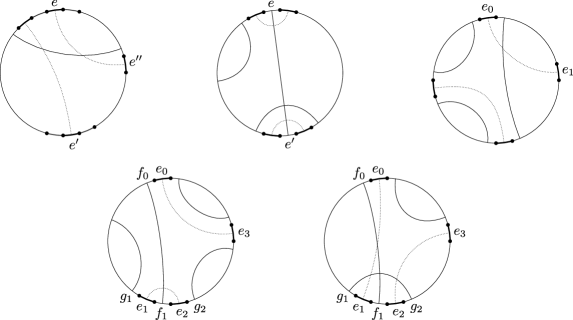
Figure C.1: The main step of the greedy algorithm. Top: (left to right) Case (a), Case (b), Case (c1). Bottom (left to right): Case (c2’), Case (c2”). For each case we draw a typical scenario, in which edges of $\gamma$ are separated by a single edge only if this is required by the case in question. The edges in $\gamma$ are drawn using thick black lines. Bridges already present in $\Gamma_{j}$ are drawn using solid lines, and bridges added by the current step using dotted lines. In Case (a), the edges in $\gamma^{\prime}$ are drawn using thick grey lines.

Let us therefore assume from now on that no two edges of $\gamma$ are adjacent. The lumping $\Gamma_{j+1}$ with marked bridges is defined according to the following four cases. (See Figure C.1 for an illustration of each case.) In each case, both properties (i) and (ii) are easy to check. (Note that, under the additional assumption $\widehat{H}_{xx}=0$ for all $x$, it is easy to see that any two edges of $\gamma$ must be separated by at least two edges, so that only Case (c1) below needs to be considered.)

• There are two edges $e,e^{\prime}\in\gamma$ whose neighbouring edges all belong to another four-lump $\gamma^{\prime}\in\Gamma_{j}$. We choose an edge $e^{\prime\prime}\in\gamma$ that has at least one neighbouring edge not in $\gamma^{\prime}$ (it is easy to see that, since $\Gamma_{j}$ cannot consist of two interlacing four-lumps by (C.1), there always exists such an $e^{\prime\prime}$). We bridge $e$ with $e^{\prime\prime}$, as well as the two remaining edges of $\gamma$ with each other. We mark the newly created bridge $\{e,e^{\prime\prime}\}$.

• There is a bridge $\{e,e^{\prime}\}\in\Gamma_{j}$ such that every edge in $\gamma$ is adjacent to either $e$ or $e^{\prime}$. We bridge both edges adjacent to $e$ with each other, as well as both edges adjacent to $e^{\prime}$ with each other. We mark the bridge $\{e,e^{\prime}\}$.

• Neither (a) nor (b) applies. We choose $e_{0}\in\gamma$ so that the set of four edges adjacent to $e_{0}$ and its two neighbours contains at most one other edge in $\gamma$. (By (C.1) such an $e_{0}$ always exists.) Define

  $$\zeta\;\mathrel{\mathop{:}}=\;\bigl{\{}{e_{1}\in\gamma\setminus\{e_{0}\}\,:\,\text{neither neighbour of $e_{1}$ is bridged in $\Gamma_{j}$ with a neighbour of $e_{0}$}}\bigr{\}}\,.$$

  • If $\zeta\neq\emptyset$, it is not hard to see that there is an $e_{1}\in\zeta$ such that the bridge $\gamma\setminus\{e_{0},e_{1}\}$ is incompatible with at most one bridge of $\Gamma_{j}$. We bridge $e_{0}$ with $e_{1}$, and both remaining edges of $\gamma$ with each other. We mark the bridge $\{e_{0},e_{1}\}$.

  • If $\zeta=\emptyset$, there is a bridge $\{f_{0},f_{1}\}\in\Gamma_{j}$ such that $f_{0}$ is adjacent to $e_{0}$, and $f_{1}$ is adjacent to two edges, $e_{1}$ and $e_{2}$; see Figure C.1. We choose $e_{2}$ to be the edge “antipodal” to $e_{0}$ in the circular ordering of the four edges of $\gamma$, i.e. $e_{2}$ is the edge that cannot be reached from $e_{0}$ along the circle without crossing another edge of $\gamma$. Clearly, one of the two selected edges has this property. Define $e_{3}\mathrel{\mathop{:}}=\gamma\setminus\{e_{0},e_{1},e_{2}\}$. Let $g_{1}\neq f_{1}$ and $g_{2}\neq f_{1}$ denote the two other neighbours of $e_{1}$ and $e_{2}$.

    • Assume first that $g_{1}$ and $g_{2}$ are not bridged in $\Gamma_{j}$. In this case we bridge $e_{1}$ with $e_{2}$ and $e_{0}$ with $e_{3}$; we mark the bridge $\{e_{1},e_{2}\}$. It is immediate that $\{e_{1},e_{2}\}$ is compatible with all bridges in $\Gamma_{j}$, and that $\{e_{0},e_{3}\}$ is incompatible with precisely one bridge in $\Gamma_{j}$.

    • Assume now that $g_{1}$ and $g_{2}$ are bridged in $\Gamma_{j}$. Then we bridge $e_{2}$ with $e_{3}$ and $e_{0}$ with $e_{1}$. We mark the bridge $\{e_{2},e_{3}\}$. Since Case (b) is excluded, we find that the bridge $\{e_{2},e_{3}\}$ is compatible with all bridges of $\Gamma_{j}$. Moreover, the bridge $\{e_{0},e_{1}\}$ is incompatible with precisely one bridge of $\Gamma_{j}$.

The pictures in Figure C.1 depict typical scenarios, in which edges of $\gamma$ are separated by a single edge (they are next-nearest neighbours) only if this is explicitly required in the case being considered. It is also possible that additional edges are next-nearest neighbours; e.g. it may happen that $f_{0}=g_{1}$ in the last picture. Checking the few such explicit cases, one can see that the algorithm described above works for these cases as well, even though the pictures are not accurate. It is this step where the special choice of $e_{0}$ made in Case (c) is necessary.

Set $j\mapsto j+1$. If $\Gamma_{j}$ is not yet a pairing, we repeat the procedure. Otherwise, we set $\Pi\mathrel{\mathop{:}}=\Gamma_{j}$ and stop the recursion; this is the completion of the algorithm. We need two crucial observations about the algorithm.

First, no bridge of $\Pi$ is marked twice. Indeed, in Cases (a) and (c), the bridge marked at step $j$ is new (i.e. does not exist in $\Gamma_{j}$); in Case (b) the bridge marked at step $j$, i.e. $\{e,e^{\prime}\}$, was unmarked in $\Gamma_{j}$, as follows from the definition of Case (a). (The marking of $\{e,e^{\prime}\}$ could only have been done in Case (a) if there $e$ had been bridged with $e^{\prime}$, but this does not happen.) Therefore, the number of marked bridges of $\Pi$ is equal to the number of steps of the algorithm, i.e. the number of four-lumps in $\Gamma^{\prime}$, which is $p(\Gamma^{\prime})/2$.

Second, no two marked bridges of $\Pi$ belong to the same (anti)ladder. Indeed, by construction, the bridge marked at step $j$ of the algorithm is compatible with all bridges of $\Gamma_{j}$. Thus, if two marked bridges of $\Pi$, $\gamma$ and $\gamma^{\prime}$, belong to the same (anti)ladder in $\Pi$, then there must exist a $j$ such that at step $j$ we added a bridge $\gamma^{\prime\prime}$ (marked or not) that was (anti)parallel to two bridges of $\Gamma_{j}$, one belonging to an (anti)ladder containing $\gamma$ and the other to an (anti)ladder containing $\gamma^{\prime}$. By construction, however, this never happens; see (ii).

In conclusion: $\Pi$ has $p(\Gamma^{\prime})/2$ marked bridges, such that no two of them lie in the same ladder or antiladder of $\Pi$. Therefore, for any choice of tags of the bridges of $\Pi$, the resulting skeleton will always contain at least $p(\Gamma^{\prime})/2$ bridges. From (C.2) we therefore get $m(\Pi)\geqslant p(\Gamma)/4$.

That $m(\Pi)\geqslant 2$ is easy to see from the fact that $m(\Pi)=1$ would imply that $\Pi$ is either a complete ladder or a complete antiladder; this never happens by the property (i) of the greedy algorithm.

Appendix D Proof of Proposition 10.7

The key to the proof Proposition 10.7 is a decoupling of the bough tagging from the bough graph. The is done by adding an appropriate number of bough edges to $G\cup G^{\prime}$, as in the proof of Lemma 9.8.

Lemma D.1.

There is an injective map $Y:\mathfrak{G}_{\sharp}\to\mathfrak{G}_{\sharp}$ such that for any $\mathcal{G}=(G,\tau_{G})$ and $\mathcal{\widetilde{G}}=(\widetilde{G},\tau_{\widetilde{G}})=Y(\mathcal{G})$ the following properties hold.

1. The tagged stems of $\mathcal{G}$ and $\widetilde{\mathcal{G}}$ are identical.

2. $\deg\bigl{(}{\mathcal{B}(G),\tau_{G}}\bigr{)}=2\lvert\mathcal{E}(\mathcal{B}(\widetilde{G}))\rvert$.

3. For any $\mathcal{G},\mathcal{G}^{\prime}\in\mathfrak{G}_{\sharp}$ we have the bound

   $$E_{\mathcal{G}\cup\mathcal{G}^{\prime}}\;\leqslant\;\Biggl{[}{\prod_{e\in\mathcal{E}_{B}\text{\rm nonleaf}}\bigl{(}{M^{-1+2\delta}}\bigr{)}^{\bm{\mathrm{1}}(\tau(e)\neq(b,0))}}\Biggr{]}\bigl{(}{CM^{-\delta}}\bigr{)}^{L^{(b)}}\bigl{(}{CM^{-1+\mu+5\delta}}\bigr{)}^{L^{(f)}}\bigl{(}{CM^{-1+\mu+7\delta}}\bigr{)}^{L^{(d)}/2}\\ \times\sum_{\widetilde{\Gamma}\in\mathscr{G}_{u,u^{\prime}}}\sum_{\bm{\mathrm{x}}_{S}\,:\,\Gamma(\bm{\mathrm{x}}_{S})=\widetilde{\Gamma}}Q(\bm{\mathrm{x}}_{S})\prod_{\gamma\in\widetilde{\Gamma}}\mathbb{E}\prod_{e\in\gamma}\Bigl{\lvert}P_{\tau(e)}\bigl{(}{\widehat{H}_{x_{a(e)}x_{b(e)}},\widehat{H}_{x_{b(e)}x_{a(e)}}}\bigr{)}\Bigr{\rvert}\,,$$ (D.1)

   where all quantities on the right-hand side of (D.1) are defined in terms of $\widetilde{\mathcal{G}}\cup\widetilde{\mathcal{G}}^{\prime}$, i.e. $L^{(i)}\equiv L^{(i)}(\widetilde{\mathcal{G}}\cup\widetilde{\mathcal{G}}^{\prime})$ for $i=b,f,d$, and $\tau\equiv\tau_{\widetilde{G}\cup\widetilde{G}^{\prime}}$.

Using Lemma D.1 we find that Proposition 10.7 follows easily by repeating to the letter the argument at the beginning of Subsection 9.5.

Proof of Lemma D.1.

For any graph $G$ we define the two following cases.

1. $\mathcal{B}(G)$ is either empty or contains at least one nondegenerate bough.

2. $\mathcal{B}(G)$ consists exclusively of degenerate boughs.

Consider first the case that both $G$ and $G^{\prime}$ satisfy (a). Then we may proceed exactly as in the proof of Lemma 9.8. Thus, we define

$$D\;\mathrel{\mathop{:}}=\;\deg\bigl{(}{\mathcal{B}(G),\tau_{G}}\bigr{)}-2\lvert\mathcal{E}(\mathcal{B}(G))\rvert\,.$$

If $D=0$ set $\widetilde{\mathcal{G}}=\mathcal{G}$. Otherwise $\mathcal{B}(G)$ contains a nondegenerate bough. Let $e$ be the nonleaf bough edge that is reached first on the walk around $G$ (see the proof of Proposition 6.6 for the definition of the walk around $G$). Define $\widetilde{\mathcal{G}}$ as $\mathcal{G}$ in which we replaced the edge $e$ with a path of $D+1$ edges; here the first edge of the path carries the tag $\tau_{G}(e)$ and all other edges of the path the tag $(b,0)$.

Now set $Y(\mathcal{G})\mathrel{\mathop{:}}=\widetilde{\mathcal{G}}$. By construction, we have that

$$L^{(b)}(\widetilde{G})\;=\;L^{(b)}(G)\,,\qquad L^{(f)}(\widetilde{G})\;=\;L^{(f)}(G)\,,\qquad L^{(d)}(\widetilde{G})\;=\;L^{(d)}(G)\,.$$

Moreover, $\mathcal{G}$ and $\mathcal{\widetilde{G}}$ have the same number of small nonleaf bough edges. It is also easy to see that Claims (i) and (ii) hold. Moreover, as in the proof of Lemma 9.8, we find that the map $\mathcal{G}\mapsto\widetilde{\mathcal{G}}$ is injective. Defining $\widetilde{\mathcal{G}}^{\prime}$ in the same way, we find that Claim (iii) follows from Proposition 10.6.

Next, consider the case where $G$ satisfies (b) and $G^{\prime}$ satisfies (a). The complication here is that we cannot add bough edges to $G$ without changing the numbers $L^{(b)},L^{(f)},L^{(d)}$. If $D=0$ then we can set $\widetilde{\mathcal{G}}=\mathcal{G}$ and proceed as above. If $D>0$ then there must be a (degenerate) bough edge $\widetilde{e}\in\mathcal{E}(\mathcal{B}(G))$ whose tag is $\tau_{G}(\widetilde{e})=(b,i)$ for $i=2,3,4$. We now use the additional small factor arising from such an edge. We claim that in this case we can improve the bound (10.19) to

$$E_{\mathcal{G}\cup\mathcal{G}^{\prime}}\;\leqslant\;\Biggl{[}{\prod_{e\in\mathcal{E}_{B}\text{\rm nonleaf}}\bigl{(}{M^{-1+2\delta}}\bigr{)}^{\bm{\mathrm{1}}(\tau(e)\neq(b,0))}}\Biggr{]}\bigl{(}{CM^{-\delta}}\bigr{)}^{L^{(b)}}\bigl{(}{CM^{-1+\mu+5\delta}}\bigr{)}^{L^{(f)}}\bigl{(}{CM^{-1+\mu+7\delta}}\bigr{)}^{(L^{(d)}-1)/2}M^{-1+2\delta}\\ \times\sum_{\widetilde{\Gamma}\in\mathscr{G}_{u,u^{\prime}}}\sum_{\bm{\mathrm{x}}_{S}\,:\,\Gamma(\bm{\mathrm{x}}_{S})=\widetilde{\Gamma}}Q(\bm{\mathrm{x}}_{S})\prod_{\gamma\in\widetilde{\Gamma}}\mathbb{E}\prod_{e\in\gamma}\Bigl{\lvert}P_{\tau(e)}\bigl{(}{\widehat{H}_{x_{a(e)}x_{b(e)}},\widehat{H}_{x_{b(e)}x_{a(e)}}}\bigr{)}\Bigr{\rvert}\,.$$ (D.2)

Note the additional factor $M^{-1+2\delta}$ at the expense of reducing the exponent of $M^{-1+\mu+7\delta}$ by 1/2. We outline the proof of (D.2), which is almost identical to the proof of (10.19). In choosing the ordering of edges $\preceq$, we require that $\widetilde{e}$ be the first degenerate bough edge. When tackling the edge $\widetilde{e}$ immediately after the recursive algorithm (used for nondegenerate boughs) of Proposition 10.5 has terminated, we get a bound $\xi=M^{-1+2\delta}=M^{-1+\mu+5\delta}M^{-\mu-3\delta}$. Here the first term is the worst-case estimate using (10.2), and the second arises from the fact that, thanks to the assumption on $\tau(\widetilde{e})$, the estimate (10.3) is now in fact valid if we multiply the right-hand side by a factor $M^{-\mu-3\delta}$. The remaining $L^{(d)}-1$ degenerate edges are estimated exactly as in Section 10.4. Thus we get (D.2).

Now we may proceed as above. Let $e$ be the (degenerate) leaf that is reached first on the walk around $G$. Define $\widetilde{\mathcal{G}}$ as $\mathcal{G}$ in which we replaced the edge $e$ with a path of $D+1$ edges; here the first edge of the path carries the tag $\tau_{G}(e)$ and all other edges of the path carry the tag $(b,0)$. Denoting by $l\geqslant 1$ the number of leaves in $G$ belonging to the bough containing $e$, we have

$$L^{(b)}(\widetilde{G})\;=\;l-1\,,\qquad L^{(f)}(\widetilde{G})\;=\;1\,,\qquad L^{(d)}(\widetilde{G})\;=\;L^{(d)}(G)-l\,.$$

These identities are simply an expression of the fact that the degenerate bough of $G$ that contains $e$ becomes a nondegenerate bough in $\widetilde{G}$ with one free leaf. Moreover, the mapping $\mathcal{G}\mapsto\widetilde{\mathcal{G}}$ clearly satisfies Claims (i) and (ii). That it is injective can be seen from the fact that $\mathcal{G}$ can be reconstructed from $\widetilde{\mathcal{G}}$, similarly to the construction given in the proof of Lemma 9.8.

Choosing $\widetilde{\mathcal{G}}^{\prime}=Y(\mathcal{G}^{\prime})$ as above, we find that the bound (D.1) follows from (D.2) and the bound

$$\bigl{(}{CM^{-1+\mu+7\delta}}\bigr{)}^{(L^{(d)}-1)/2}M^{-1+2\delta}\;\leqslant\;\bigl{(}{CM^{-\delta}}\bigr{)}^{l-1}CM^{-1+\mu+5\delta}\bigl{(}{CM^{-1+\mu+7\delta}}\bigr{)}^{(L^{(d)}-l)/2}\,,$$

which is easy to check for all $l\geqslant 1$.

Finally, the case when both $G$ and $G^{\prime}$ satisfy (b) is dealt with exactly as the previous case. ∎

Appendix E List of concepts and symbols

graph $G,G^{\prime},\dots$	A rooted, oriented, unlabelled tree graph; see p. 6.3.
stem $\mathcal{S}(G)$ of a graph $G$	The path of $G$ joining the vertices $a(G)$ and $b(G)$; see p. 6.3.
boughs $\mathcal{B}(G)$ of a graph $G$	The subgraph of $G$ that does not contain the stem of $G$; a collection of disjoint trees; see p. 6.3.
tagging $\tau$	A map from the edges of a graph to the set of tags encoding the contribution of an edge; see p. 6.3 as well as Figures 6.4 and 6.5.
nonbacktracking encoding $l$	A map assigning to each pair of vertices $v,w$ a number $l(v,w)=0,1$, used to encode any nonbacktracking conditions; see p. 6.7.
decorated graph $\mathcal{G},\mathcal{G}^{\prime},\dots$	A graph $G$ together with a tagging $\tau_{G}$ of $G$ and a map $l_{G}$ implementing any nonbacktracking conditions; see p. 6.7.
label $x_{v}$ of a vertex $v$	An element $x_{v}\in\Lambda_{N}$ assigned to $v$; see p. 6.3.
lumping $\Gamma$	An equivalence relation on the set of edges arising from taking the expectation value; see p. 7.3.
pairing $\Pi$	The simplest type of lumping, whose equivalence classes each consist of two edges; see p. 8.1.
bridge $\pi$	A lump of a pairing; see p. 8.1.
(anti)parallel bridges	See p. 8.2.
twisted and straight bridges	See p. 8.1.
tagged pairing $(\Pi,\theta)$	A pairing $\Pi$ whose bridges $\pi$ carry a tag $\vartheta(\pi)\in\{\text{straight, twisted}\}$; see p. 8.4.
ladder $L_{n}$	The simplest pairing, whose contribution is of leading order; see p. 8.3.
skeleton pairing $S(\Pi,\vartheta)$	Tagged pairing obtained from the tagged pairing $(\Pi,\vartheta)$ by collapsing parallel straight bridges and antiparallel twisted bridges; see p. 8.2.
lonely leaf	A leaf that is the only edge of its lump; see Definition 9.5.
degenerate, bound, free leaves	See Definition 10.2.
$\mathfrak{W}$	The set of graphs; see p. 6.3 and Figure 6.3.
$\mathfrak{G}$	The set of decorated graphs; see p. 6.7.
$\mathfrak{G}^{\prime}$	The set of decorated graphs corresponding to terms of the main path expansion (6.4); see Definition 6.4.
$\mathfrak{V}_{xy}(\mathcal{G})$	The value of the decorated graph, a random variable; see (6.9).
$\mathcal{F}_{n}$	The operation that makes nonbacktracking the first backtracking stem vertex of a decorated graph; see p. 6.4.
$\mathcal{F}_{c}$	The operation that collapses the two stem neighbours of the first backtracking stem vertex of a decorated graph; see p. 6.4.
$\mathscr{B}_{\mathcal{G}}$	The set of decorated graphs obtained from $\mathcal{G}\in\mathfrak{G}^{\prime}$ by applying the operations $\mathcal{F}_{n},\mathcal{F}_{n}$ until the stem is completely nonbacktracking; see Definition 6.5.
$\mathfrak{G}_{\sharp}$	The union of all $\mathscr{B}_{\mathcal{G}}$ for $\mathcal{G}\in\mathfrak{G}^{\prime}$; see Definition 6.5.
$\deg(\mathcal{G})$	The degree of the decorated graph $\mathcal{G}$, representing the degree of the polynomial $\mathfrak{V}_{xy}(\mathcal{G})$; see p. 6.3.
$\mathfrak{G}_{n}$	The set of decorated graphs in $\mathfrak{G}_{\sharp}$ of degree $n$; see p. 6.13.
$\mathscr{G}(G\cup G^{\prime})$	The set of lumpings of the edges of $G\cup G^{\prime}$; see p. 7.5.
$I_{n}$	The graph in $\mathfrak{W}$ that consists of a bare stem with $n$ edges; see p. 7.
$\mathcal{I}_{n}$	The decorated graph in $\mathfrak{G}_{n}$ obtained by assigning the tag $(s,0)$ to all edges of $I_{n}$; see p. 7.
$\mathfrak{G}^{*}_{n}$	The set $\mathfrak{G}_{n}\setminus\{\mathcal{I}_{n}\}$; see p. 7.
$\mathscr{G}_{n,n^{\prime}}$	An abbreviation for $\mathscr{G}(I_{n}\cup I_{n^{\prime}})$; see p. 7.
$\mathscr{P}_{n,n^{\prime}}$	The subset of $\mathscr{G}_{n,n^{\prime}}$ consisting of pairings; see p. 8.1.
$V_{x}(\mathcal{G}\cup\mathcal{G}^{\prime},\Gamma)$	The value of the lumping $\Gamma\in\mathscr{G}(G\cup G^{\prime})$ of the edges of the decorated graph $\mathcal{G}\cup\mathcal{G}^{\prime}$; see (7.6).
$\preceq$	A total order on the edges of $G\cup G^{\prime}$ describing the order used for summing out bough vertices; see pp. 9.2 and 10.2.
$A$	A map that assigns to each bough edge $e$ an edge $A_{e}\succeq e$, and is used to parametrize the lumping of the bough edges; see p. 9.2.

References

- [1] Erdős, L. and Knowles, A.: Quantum diffusion and eigenfunction delocalization in a random band matrix model, Preprint arXiv:1002.1695, to appear in Comm. Math. Phys.
- [2] Feldheim, O. and Sodin, S.: A universality result for the smallest eigenvalues of certain sample covariance matrices, Geom. Funct. Anal. 20 (2010), no. 1, 88-123.
- [3] Anderson, G., Guionnet, A., Zeitouni, O.: An Introduction to Random Matrices. Studies in advanced mathematics, 118, Cambridge University Press, 2009.
- [4] Khorunzhiy, O.: Estimates for moments of random matrices with Gaussian elements, Séminaire de probabilités XLI, 51–92, Lecture Notes in Math. 1934, Springer, 2008.
- [5] Sodin, S.: The spectral edge of some random band matrices, Ann. of Math. (2) 172 (2010), no. 3, 2223-2251.
- [6] Soshnikov, A.: Universality at the edge of the spectrum in Wigner random matrices, Comm. Math. Phys. 207 (1999), no. 3, 697-733.
- [7] Stanley, R. P.: Enumerative combinatorics, Vol. 2, Cambridge University Press, 1999.
- [8] Stroock, D.: Probability theory, and analytic view, Cambridge University Press, 1999.
- [9] Vu, V.: Spectral norm of random matrices, Combinatorica 27 (2007), no. 6, 721-736.