Universal Quantum Computation Using Continuous Dynamical Decoupling

Abstract

We show, for the first time, that continuous dynamical decoupling can preserve the coherence of a two-qubit state as it evolves during a $\sqrt{\rm SWAP}$ quantum operation. Hence, because the Heisenberg exchange interaction alone can be used for achieving universal quantum computation, its combination with continuous dynamical decoupling can also make the computation robust against general environmental perturbations. Furthermore, since the exchange-interaction Hamiltonian is invariant under rotations, the same control-field arrangement used to protect a stationary quantum-memory state can also preserve the coherence of the driven qubits. The simplicity of the required control fields greatly improves prospects for an experimental realization.

Quantum computers use superposition and entanglement of qubits to outperform digital computers deutsch92 . The advent of these machines will unquestionably encompass a radical transformation in the way we simulate quantum-mechanical processes feynman82 , imparting a plethora of new achievements in science and technology. However, the benefits of reliable quantum information processing depend on the development of efficient ways to avoid or recover from qubit errors induced by environmental interaction zurek03 .

A universal set of quantum gates consists of arbitrary single-qubit coherent rotations and a particular entangling operation divincenzo95 . Such a two-qubit unitary operation is the $\sqrt{\rm SWAP}$ gate, that has recently been realized experimentally using double quantum dots petta05 and neutral atoms in an optical lattice anderlini07 . An ideal $\sqrt{\rm SWAP}$ gate is obtained by the Heisenberg coupling between two qubits, whose dynamics is governed by the Hamiltonian

$$H_{0}=J{\bm{\sigma}}^{(1)}\cdot{\bm{\sigma}}^{(2)},$$ (1)

where we use $\hbar=1$ throughout, $J$ is the exchange constant, and, for $s=1,2$, ${\bm{\sigma}}^{(s)}={\bf\hat{x}}\sigma_{x}^{(s)}+{\bf\hat{y}}\sigma_{y}^{(s)}+{\bf\hat{z}}\sigma_{z}^{(s)}$, where $\sigma_{x}^{(s)}$, $\sigma_{y}^{(s)}$, and $\sigma_{z}^{(s)}$ are the Pauli matrices acting on qubit $s$. Remarkably, it has been shown that the Heisenberg interaction alone is enough for universal quantum computation, without the need of supplementary single-qubit operations divincenzo00 . Thus, a protective scheme for quantum gates such as the $\sqrt{\rm SWAP}$ is of fundamental importance, since any quantum computation can be based solely on the exchange interaction.

Here we show, for the first time, the effectiveness of dynamical decoupling to protect the $\sqrt{\rm SWAP}$ quantum-gate operation on physical qubits, during a dynamical evolution subject to a noisy environment. Our procedure admits, not only pulsed, but also continuous control Hamiltonians and, in fact, can culminate in a better protection clausen . Since the Heisenberg interaction is given by a scalar product, it is invariant under rotations. The implication of such a rotation invariance is that a simple field arrangement suffices to protect, simultaneously, not only the $\sqrt{\rm SWAP}$ quantum-gate operation, but also a quantum memory. Furthermore, the protection thus achieved is against general classes of errors, granting increased chances of successful experiments.

In a previous work, we have shown that it is possible to use a continuously-applied external field to protect entangled states from errors caused by the unavoidable interactions between the qubit system and its environment fanchini07 . The question naturally arises as to whether it is also possible to protect an entangling operation. Here we show that the very same external-field configuration of Ref. fanchini07 can prevent errors from occurring during the application of a $\sqrt{\rm SWAP}$ quantum gate. In other words, we show that if the control Hamiltonian is written as

$$H_{c}(t)={\bm{\Omega}}(t)\cdot\left({\bm{\sigma}}^{(1)}+{\bm{\sigma}}^{(2)}\right),$$ (2)

then the dynamics is protected by the field arrangement given by

$${\bm{\Omega}}(t)={\bf\hat{x}}n_{x}\omega+n_{z}\omega\left[{\bf\hat{z}}\cos\left(n_{x}\omega t\right)-{\bf\hat{y}}\sin\left(n_{x}\omega t\right)\right],$$ (3)

where $\omega=2\pi/t_{c}$, $n_{x}$ and $n_{z}\neq n_{x}$ are non-zero integers, and $t_{c}$ is a constant. This is a simple combination of a static field along the $x$ axis and a rotating field in the $yz$ plane. Moreover, addressing each qubit independently is not necessary; the field is supposed to be spatially uniform in the neighborhood surrounding both qubits.

The evolution operator associated with the control Hamiltonian is as in Ref. fanchini07 :

$$U_{c}(t)=U^{(2)}(t)U^{(1)}(t)=U^{(1)}(t)U^{(2)}(t),$$ (4)

since ${\bm{\sigma}}^{(1)}$ and ${\bm{\sigma}}^{(2)}$ commute, where

$$U^{(s)}(t)=\exp\left(-i\omega tn_{x}\sigma_{x}^{(s)}\right)\exp\left(-i\omega tn_{z}\sigma_{z}^{(s)}\right),$$ (5)

for $s=1,2$. Because Eq. (1) is a scalar product, it is invariant under rotations and $U^{\dagger}_{c}(t)H_{0}U_{c}(t)=H_{0}$. This property of the Heisenberg interaction tremendously simplifies the quantum operations executed under the protection by continuous dynamical decoupling. If it were not for this rotational invariance, we would have to proceed as in Ref. fanchini022329 and introduce an auxiliary rotating reference frame, complicating the procedure. Furthermore, this invariance has another peculiarity: the same field arrangement that can preserve a quantum memory, can also, with exactly the same configuration, protect the quantum-gate operation. No reconfiguration of fields being necessary during the gate operation is a tremendous simplification; it certainly improves the prospects for experimental realization.

To illustrate our protective scheme, we begin by assuming that the interaction Hamiltonian between the qubit system and the rest of the universe is of the form

$$H_{\rm int}={\bf B}^{(1)}\cdot{\bm{\sigma}}^{(1)}+{\bf B}^{(2)}\cdot{\bm{\sigma}}^{(2)},$$ (6)

where ${\bf B}^{(s)}=\sum_{m=1}^{3}B_{m}^{(s)}{\bf\hat{x}}_{m}$, for $s=1,2$, with ${\bf\hat{x}}_{1}\equiv{\bf\hat{x}}$, ${\bf\hat{x}}_{2}\equiv{\bf\hat{y}}$, ${\bf\hat{x}}_{3}\equiv{\bf\hat{z}}$, and $B_{m}^{(s)}$, for $s=1,2$ and $m=1,2,3$, are Hermitian operators that act on the environmental Hilbert space. It follows from Eqs. (4), (5), and (6) that $U_{c}(t)$ satisfies the requirement for dynamical decoupling DD :

$$\int^{t_{c}}_{0}U^{\dagger}_{c}(t)H_{\rm int}U_{c}(t)dt=0,$$ (7)

where $t_{c}=2\pi/\omega$. In order to control the intensity of the exchange interaction, possible candidates for the physical qubits should be, for example, properly built tunable charge qubits schon . Although, in this particular case, physical reasoning leads us to assume that each qubit is coupled to its own environment, we shall, for the sake of completeness, also study the case of a common environment. For our present purposes, we assume that the particular form of Eq. (6) is, in the case of a common environment, given by

$$H_{int}=\left({\bm{\sigma}}^{(1)}+{\bm{\sigma}}^{(2)}\right)\cdot\left({\bm{\lambda}}B+{\bm{\lambda}}^{\ast}B^{\dagger}\right),$$ (8)

where ${\bm{B}}^{(s)}={\bm{\lambda}}B+{\bm{\lambda}}^{\ast}B^{\dagger}$, for $s=1,2$, ${\bm{\lambda}}$ is an arbitrary complex three-dimensional vector, and $B$ is a scalar operator that acts on the environmental Hilbert space. However, when the qubits are physically located sufficiently far apart, as for tunable charge qubits schon , it is reasonable to suppose that their individual surroundings act as uncorrelated, independent environments. In that case, the particular form we assume for Eq. (6) is written as

$$H_{int} = {\bm{\sigma}}^{(1)}\cdot\left({\bm{\lambda}^{(1)}}B^{(1)}+{\bm{\lambda}^{(1)}}^{\ast}{B^{(1)}}^{\dagger}\right)$$ (9)

$$+ {\bm{\sigma}}^{(2)}\cdot\left({\bm{\lambda}^{(2)}}B^{(2)}+{\bm{\lambda}^{(2)}}^{\ast}{B^{(2)}}^{\dagger}\right)$$

where $B^{(s)}$, for $s=1,2$, acts on the environmental Hilbert space of the $s$-th qubit, and ${\bm{\lambda}^{(s)}}$ is an arbitrary complex three-dimensional vector for $s=1,2$.

We first consider the point of view of the picture defined by the unitary transformation $U_{c}(t)$; thus, the total Hamiltonian can be written

$$H(t)=H_{0}+H_{E}+U^{\dagger}_{c}(t)H_{\rm int}U_{c}(t),$$ (10)

where $H_{E}$ is the environmental Hamiltonian and, therefore, $U^{\dagger}_{c}(t)H_{E}U_{c}(t)=H_{E}$. We represent the environment of each qubit as a thermal bath of harmonic oscillators. In the case of a common environment for both qubits, we consider $H_{E}=\sum_{k}\omega_{k}{a_{k}}^{\dagger}a_{k}$, where $\omega_{k}$ is the frequency of the $k$-th normal mode of the common environment, and $a_{k}$ and ${a_{k}}^{\dagger}$ are the annihilation and creation operators, respectively. In the case of two independent and identical environments, instead of above we take $H_{E}=\sum_{s=1}^{2}\sum_{k}\omega_{k}{a_{k}^{(s)}}^{\dagger}a_{k}^{(s)}$, where $\omega_{k}$ is the frequency of the $k$-th normal mode of the $s$-th qubit environment, and $a_{k}^{(s)}$ and ${a_{k}^{(s)}}^{\dagger}$ are, respectively, the annihilation and creation operators. The frequency $\omega_{k}$ is the same for both independent and identical environments. Accordingly, we take $B_{m}^{(s)}=\sum_{k}\left(\lambda_{m}g_{k}^{\ast}a_{k}^{(s)}+\lambda_{m}^{\ast}g_{k}a_{k}^{(s)\dagger}\right)$,where $g_{k}$ are coupling constants.

Starting from $H(t)$, the Hamiltonian in the “interaction” picture is defined as

$$H_{I}(t)=\sum_{s=1}^{2}\sum_{m=1}^{3}\sum_{n=1}^{3}R_{m,n}(t)E_{m}^{(s)}(t)\widetilde{\sigma}_{n}^{(s)}(t).$$ (11)

where $\sigma_{1}^{(s)}\equiv\sigma_{x}^{(s)}$, $\sigma_{2}^{(s)}\equiv\sigma_{y}^{(s)}$, $\sigma_{3}^{(s)}\equiv\sigma_{z}^{(s)}$, $\widetilde{\sigma}_{n}^{(s)}(t)=U^{\dagger}_{0}(t)\sigma_{n}^{(s)}U_{0}(t)$, for $s=1,2$ and $n=1,2,3$, with $U_{0}(t)=\exp(-iH_{0}t)$. We have used Eq. (6) and defined the operators $E_{m}^{(s)}(t)=U^{\dagger}_{E}(t)B_{m}^{(s)}U_{E}(t)$, for $s=1,2$ and $m=1,2,3$, with $U_{E}(t)=\exp(-iH_{E}t)$. The quantities $U^{\dagger}_{c}(t)\sigma_{m}^{(s)}U_{c}(t)=\sum_{n=1}^{3}R_{m,n}(t)\sigma_{n}^{(s)}$, for $s=1,2$ and $m=1,2,3$, are rotations of $\sigma_{m}^{(s)}$, whose matrix elements, $R_{m,n}(t)$, are real functions of time. We proceed as in Ref. fanchini07 and assume that the absolute temperature is the same in the surroundings of both qubits and these qubits, as well as their respective environments, are identical. We then write down the master equation for the two-qubit reduced density matrix, $\rho_{I}(t)$, in the Born approximation:

$$\frac{d\rho_{I}(t)}{dt} = \sum_{s,s^{\prime}=1}^{2}\sum_{n,n^{\prime}=1}^{3}\int_{0}^{t}dt^{\prime}\,\left\{\mathcal{D}_{n,n^{\prime}}^{(s,s^{\prime})}(t,t^{\prime})[\widetilde{\sigma}_{n}^{(s)}(t),\rho_{I}(t)\widetilde{\sigma}_{n^{\prime}}^{(s^{\prime})}(t^{\prime})]+[\mathcal{D}_{n,n^{\prime}}^{(s,s^{\prime})}(t,t^{\prime})]^{*}[\widetilde{\sigma}_{n^{\prime}}^{(s^{\prime})}(t^{\prime})\rho_{I}(t),\widetilde{\sigma}_{n}^{(s)}(t)]\right\},$$ (12)

where we have define the coefficients

$$\mathcal{D}_{n,n^{\prime}}^{(s,s^{\prime})}(t,t^{\prime}) = \sum_{m=1}^{3}\sum_{m^{\prime}=1}^{3}R_{m,n}(t)R_{m^{\prime},n^{\prime}}(t^{\prime})C_{m,m^{\prime}}^{(s,s^{\prime})}(t,t^{\prime}),$$

for $n,n^{\prime}=1,2,3$ and $s,s^{\prime}=1,2$, and

$$C_{m,m^{\prime}}^{(s,s^{\prime})}(t,t^{\prime}) = \mathrm{Tr}_{E}\left\{E_{m}^{(s)}(t)\rho_{E}E_{m^{\prime}}^{(s^{\prime})}(t^{\prime})\right\},$$

for $m,m^{\prime}=1,2,3$ and $s,s^{\prime}=1,2$. $C_{m,m^{\prime}}^{(s,s^{\prime})}(t,t^{\prime})$ is the correlation function between components $m$ and $m^{\prime}$ of environmental operators calculated at the same qubit position, as explained in Ref. fanchini07 . Here, $\mathrm{Tr}_{E}$ denotes the trace over the environmental degrees of freedom. The operators $\widetilde{\sigma}_{n}^{(s)}(t)$, for $s=1,2$ and $n=1,2,3$, can be explicitly obtained as the components of the following vector relations:

$$U^{\dagger}_{0}(t){\bm{\sigma}}^{(1)}U_{0}(t)=a(t){\bm{\sigma}}^{(1)}+b(t){\bm{\sigma}}^{(2)}$$

$$-c(t)({\bm{\sigma}}^{(1)}\times{\bm{\sigma}}^{(2)}),$$ (13)

and

$$U^{\dagger}_{0}(t){\bm{\sigma}}^{(2)}U_{0}(t)=a(t){\bm{\sigma}}^{(2)}+b(t){\bm{\sigma}}^{(1)}$$

$$-c(t)({\bm{\sigma}}^{(2)}\times{\bm{\sigma}}^{(1)}),$$ (14)

where $a(t)=[1+\cos(4Jt)]/2$, $b(t)=[1-\cos(4Jt)]/2$, and $c(t)=\sin(4Jt)/2$. The environmental density matrix, $\rho_{E}$, is taken as the one for a canonical ensemble constituting a thermal bath, that is, $\rho_{E}=\frac{1}{Z}\exp(-\beta H_{E})$,where $Z$ is the partition function, $Z={\mathrm{T}r}_{E}\left[\exp(-\beta H_{E})\right]$. Here, $\beta=1/k_{B}T$, $k_{B}$ is the Boltzmann constant, and $T$ is the absolute temperature of the environment.

We can also write the correlation function as

$$C_{m,m^{\prime}}^{(s,s^{\prime})}(t,t^{\prime}) = \Gamma^{(s,s^{\prime})}\mathrm{Tr}_{E}\left\{E_{m}^{(s)}(t)\rho_{E}E_{m^{\prime}}^{(s)}(t^{\prime})\right\},$$

where $\Gamma^{(s,s^{\prime})}=1$ for the case of a single, common environment, in which case the environmental operators $E_{m}^{(s)}(t)$ are independent of $s$, and $\Gamma^{(s,s^{\prime})}=\delta_{s,s^{\prime}}$ for the case of two identical, uncorrelated environments. Since we have

$$E_{m}^{(s)}(t) = \sum_{k}\left[\lambda_{m}g_{k}^{\ast}a_{k}^{(s)}e^{-i\omega_{k}t}+\lambda_{m}^{\ast}g_{k}a_{k}^{(s)\dagger}e^{+i\omega_{k}t}\right]$$

and, therefore,

$$\mathrm{Tr}_{E}\!\!\left\{\!E_{m}^{(s)}(t)\rho_{E}E_{m^{\prime}}^{(s)}(t^{\prime})\!\right\}\! = \!\lambda_{m}\lambda_{m^{\prime}}^{\ast}\sum_{k}\left|g_{k}\right|^{2}n_{k}e^{-i\omega_{k}(t-t^{\prime})}$$

$$+\,\lambda_{m}^{\ast}\lambda_{m^{\prime}}\sum_{k}\left|g_{k}\right|^{2}(1+n_{k})e^{i\omega_{k}(t-t^{\prime})},$$

where $n_{k}=1/[\exp(\beta\omega_{k})-1]$, we obtain

$$\frac{d\rho_{I}(t)}{dt} = \sum_{s,s^{\prime}=1}^{2}\int_{0}^{t}dt^{\prime}\,\mathcal{T}_{1}^{(s,s^{\prime})}(t-t^{\prime})[\mathcal{R}^{(s)}(t),\rho_{I}(t)[\mathcal{R}^{(s^{\prime})}(t^{\prime})]^{\dagger}]+\sum_{s,s^{\prime}=1}^{2}\int_{0}^{t}dt^{\prime}\,\mathcal{T}_{2}^{(s,s^{\prime})}(t-t^{\prime})[[\mathcal{R}^{(s)}(t)]^{\dagger},\rho_{I}(t)\mathcal{R}^{(s^{\prime})}(t^{\prime})]$$

$$+ \sum_{s,s^{\prime}=1}^{2}\int_{0}^{t}dt^{\prime}\,[\mathcal{T}_{1}^{(s,s^{\prime})}(t-t^{\prime})]^{*}[\mathcal{R}^{(s^{\prime})}(t^{\prime})\rho_{I}(t),[\mathcal{R}^{(s)}(t)]^{\dagger}]+\sum_{s,s^{\prime}=1}^{2}\int_{0}^{t}dt^{\prime}\,[\mathcal{T}_{2}^{(s,s^{\prime})}(t-t^{\prime})]^{*}[[\mathcal{R}^{(s^{\prime})}(t^{\prime})]^{\dagger}\rho_{I}(t),\mathcal{R}^{(s)}(t)]$$

where

$$\mathcal{R}^{(s)}(t) = \sum_{m=1}^{3}\sum_{n=1}^{3}\lambda_{m}R_{m,n}(t)\widetilde{\sigma}_{n}^{(s)}(t),$$

$$\mathcal{T}_{1}^{(s,s^{\prime})}(t) = \Gamma^{(s,s^{\prime})}\sum_{k}\left|g_{k}\right|^{2}n_{k}\exp(-i\omega_{k}t),$$

and

$$\mathcal{T}_{2}^{(s,s^{\prime})}(t) = \Gamma^{(s,s^{\prime})}\sum_{k}\left|g_{k}\right|^{2}(1+n_{k})\exp(i\omega_{k}t).$$

In the limit in which the number of environmental normal modes per unit frequency becomes infinite, we define a spectral density as $J(\omega)=\sum_{k}|g_{k}|^{2}\delta(\omega-\omega_{k})$, with $\omega\in\left[0,\infty\right)$, and interpret the summations in $\mathcal{T}_{1}^{(s,s^{\prime})}(t)$ and $\mathcal{T}_{2}^{(s,s^{\prime})}(t)$ as integrals over $\omega$:

$$\mathcal{T}_{1}^{(s,s^{\prime})}(t) = \Gamma^{(s,s^{\prime})}\int_{0}^{\infty}d\omega J(\omega)\frac{\exp(-i\omega t)}{\exp(\beta\omega)-1},$$

and

$$\mathcal{T}_{2}^{(s,s^{\prime})}(t) = \left[\mathcal{T}_{1}^{(s,s^{\prime})}(t)\right]^{\ast}+\Gamma^{(s,s^{\prime})}\int_{0}^{\infty}d\omega J(\omega)\exp(i\omega t),$$

for $s,s^{\prime}=1,2$. Here we assume an ohmic spectral density with a cutoff frequency $\omega_{c}$, namely, $J(\omega)=\eta\omega\exp(-\omega/\omega_{c})$, where $\eta$ is a dimensionless constant.

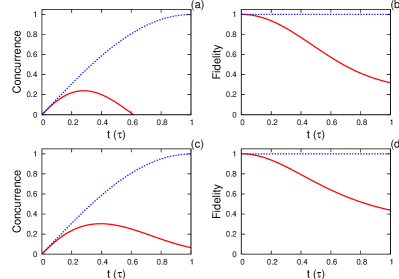
Figure 1: (Color Online) Amplitude Damping plus Dephasing: In figures (a) and (b), we show, respectively, the concurrence and the fidelity for independent environments and, in figures (c) and (d), for the common environments. The dotted (blue) line and solid (red) line represent the dynamics of a $\sqrt{\rm{SWAP}}$ quantum gate, with and without protection, respectively.

To illustrate our method, we consider the protection of an entangling operation. We take $J=\pi/8$ in Eq. (1) and assume that the two qubits are coupled to ohmic environments at $T=0.2K$, with the coupling constant $\eta=1/20$, and the cut-off frequency given by $\omega_{c}\tau=2\pi$, where $\tau=10^{-9}$s. We consider two uncorrelated classes of errors: amplitude damping and dephasing. We suppose that $\rho(0)=|\!\!\uparrow\downarrow\rangle\langle\uparrow\downarrow\!\!|$ and, in Fig. (1), we show the fidelities and the concurrences concurrence for the protected and unprotected cases of the $\sqrt{\rm SWAP}$ quantum gate. We consider that the qubits interact with independent or common environments. For the protected cases, we take $n_{x}=28\pi/\tau$ and $n_{z}=14\pi/\tau$. We observe, in all protected cases, higher fidelities and concurrences, as compared to the unprotected cases. In all examples shown in Fig. (1), the final fidelities and concurrences of the protected dynamics are near unity. In fact, in the protected cases shown, they are greater than $0.998$ and higher values can be obtained for greater values of $n_{x}$ and $n_{z}$.

To summarize, we present a simplified method to protect a $\sqrt{{\rm SWAP}}$ quantum gate from general classes of errors. Our scheme protects the logical operation at the same time as it is applied and, using the same control-field arrangement, can protect a quantum memory or a quantum gate. The flexibility of using the same control field, in the static and dynamic situations, greatly improves the prospects for an experimental realization. Furthermore, since the quantum gates derived from the exchange interaction alone are universal per se, our methodology provides the possibility of a totally-protected universal quantum computation, using continuous dynamical decoupling.

This work has been partly supported by “Fundação de Amparo à Pesquisa do Estado de São Paulo (FAPESP)”, Brazil, project number 05/04105-5, and by FAPESP and “Conselho Nacional de Desenvolvimento Científico e Tecnológico (CNPq)”, Brazil, through the “Instituto Nacional de Ciência e Tecnologia em Informação Quântica (INCT-IQ)”.

References

• (1) D. Deutsch and R. Jozsa, Proc. R. Soc. London Ser. A 439, 553 (1992); P. W. Shor, in Proceedings, 35th Annual Symposium on the Foundations of Computer Science, edited by S. Goldwasser (IEEE Computer Society Press, Los Alamitos, 1994), p. 124.
• (2) R. P. Feynman, Int. J. Theor. Phys. 21, 467 (1982).
• (3) W. H. Zurek, Phys. Today 44, 36 (1991); arXiv:quant-ph/0306072v1 (2003).
• (4) D. P. DiVincenzo, Phys. Rev. A 51 1015 (1995).
• (5) J. R. Petta, A. C. Johnson, J. M. Taylor, E. A. Laird, A. Yacoby, M. D. Lukin, C. M. Marcus, M. P. Hanson, and A. C. Gossard, Science 309, 2180 (2005).
• (6) M. Anderlini, P. J. Lee, B. L. Brown, J. Sebby-Strabley, W. D. Phillips, and J. V. Porto, Nature 448 452 (2007).
• (7) D. P. DiVincenzo, D. Bacon, J. Kempe, G. Burkard, and K. B. Whaley, Nature 408, 339 (2000).
• (8) J. Clausen, G. Bensky, and G. Kurizki, Phys. Rev. Lett. 104, 040401 (2010).
• (9) F. F. Fanchini and R. d. J. Napolitano, Phys. Rev. A 76, 062306 (2007).
• (10) F. F. Fanchini, J. E. M. Hornos, and R. d. J. Napolitano, Phys. Rev. A 75, 022329 (2007).
• (11) L. Viola and S. Lloyd, Phys. Rev. A 58, 2733 (1998); L. Viola, E. Knill, and S. Lloyd, Phys. Rev. Lett. 82, 2417 (1999); P. Facchi, S. Tasaki, S. Pascazio, H. Nakazato, A. Tokuse, and D. A. Lidar, Phys. Rev. A 71, 022302 (2005).
• (12) Y. Makhlin, G. Schön, and A. Shnirman, Rev. Mod. Phys. 73, 357 (2001).
• (13) N. H. F. Shibata and Y. Takahashi, J. Stat. Phys. 17, 171 (1977); S. Chaturvedi and J. Shibata, Z. Phys. B 35, 297 (1979).
• (14) M. A. Nielsen and I. L. Chuang, Quantum Computation and Quantum Information (Cambridge University Press, Cambridge, England, 2000).
• (15) W. K. Wootters, Phys. Rev. Lett. 80, 2245 (1998).