Directly estimating non-classicality

Abstract

We establish a method of directly measuring and estimating non-classicality—operationally defined in terms of the distinguishability of a given state from one with a positive Wigner function. It allows to certify non-classicality, based on possibly much fewer measurement settings than necessary for obtaining complete tomographic knowledge, and is at the same time equipped with a full certificate. We find that even from measuring two conjugate variables alone, one may infer the non-classicality of quantum mechanical modes. This method also provides a practical tool to eventually certify such features in mechanical degrees of freedom in opto-mechanics. The proof of the result is based on Bochner’s theorem characterizing classical and quantum characteristic functions and on semi-definite programming. In this joint theoretical-experimental work we present data from experimental optical Fock state preparation, demonstrating the functioning of the approach.

Where is the “boundary” between classical and quantum physics? Unsurprisingly, acknowledging that quantum mechanics is the fundamental theory from which classical properties should emerge in one way or the other, instances of this question have a long tradition in physics. Possibly the most conservative and stringent criterion for non-classicality of a quantum state of bosonic modes is that the Wigner function—the closest analogue to a classical probability distribution in phase space—is negative, and can hence no longer be interpreted as a classical probability distribution Wigner ; Leonhardt ; Zyc . From this, negativity of other quasi-probability distributions, familiar in quantum optics, such as the $P$-function Wigner ; Vogel follows. In fact, a lot of experimental progress was made in recent years on preparing quantum states of light modes that exhibit such non-classical features, when preparing number states, photon subtracted states, or small Schrödinger cat states Rauschenbeutel ; Ourjoumtsev06 ; Polzik . At the same time, a lot of effort is being made of driving mesoscopic mechanical degrees of freedom into quantum states eventually showing such non-classical features Optomechanics . All this poses the question, needless to say, of how to best and most accurately certify and measure such features.

In this work, (I) we demonstrate that, quite remarkably, non-classicality in the above sense can be detected from mere measurements of two conjugate variables. For a single mode, this amounts to position and momentum detection, as can be routinely done by homodyne measurements in optical systems. (II) What is more, using such data (or also data that are tomographically complete) one can get a direct and rigorous lower bound to the probability of operationally distinguishing this quantum state from one with a positive Wigner function—including a full certificate. Such a bound uses information from possibly much fewer measurement settings than needed for full quantum state tomography. At the same time, quantum state tomography using Radon transforms for quantum modes is overburdened with problems of ill-conditioning: This gives, strictly speaking, rise to the situation that when fully reconstructing a state based on such tomographically complete data, one often should expect to encounter such large error bars that the resulting state would well be also consistent with having had no non-classicality at all.

The method introduced here, in contrast, is a direct method giving rise to a certified bound which arises from conditions all classical and quantum characteristic functions have to satisfy as being grasped by the classical and quantum Bochner’s theorem Hudson . Hence, we ask: “What is the least non-classical state consistent with the data”? Intuitively speaking, the proof circles around the deviation of a quantum characteristic function as the Fourier transform of the Wigner function from a classical characteristic function. This deviation can then be formulated in terms of a semi-definite program—so a well-behaved convex optimization problem—giving rise to certifiable bounds. The same technique can also be applied to notions of entanglement, and indeed, the rigor applied here reminds of applying quantitative entanglement witnesses. In this sense, one can directly certify quantum properties with much less than full tomographic knowledge. What is more, the criterion evaluation procedure is efficient. At present, such techniques should be most applicable to systems in quantum optics, and we indeed implement this idea in a quantum optical experiment preparing a field mode in a non-classical state. Yet, they should be expected to be helpful when eventually certifying that a mesoscopic mechanical system has eventually reached quantum properties Optomechanics , where “having achieved a non-classical state”, with careful error analysis, will constitute an important benchmark.

Measure of non-classicality. – Non-classicality is most reasonably quantified in terms of the possibility of operationally distinguishing a given state from a state that one would conceive as being classical. That is to say, the meaningful notion of distinguishing a state from a classical one is as follows.

Definition 1 (Measure of non-classicality)

Non-classicality is measured in terms of the operational distinguishability of a given state from a state having a positive Wigner function,

$$\eta(\rho)=\min_{\omega\in\mathcal{C}}\|\rho-\omega\|_{1}$$ (1)

where $\mathcal{C}$ denotes the set of all quantum states with positive Wigner function and $\|\cdot\|_{1}$ is the trace norm.

This measure is indeed the operational definition of a non-classical state—as long as one accepts the negativity of the Wigner function as the figure of merit of non-classicality. Needless to say, the operational distinguishability with respect to other properties would also be quantified by trace-distances, and naturally several quantities of such a type can be found in the literature (see, e.g., Ref. measure ). By definition, it has among others the following natural properties:

(a) It is invariant under passive and active linear transformations.

(b) It is non-increasing under Gaussian channels, and in fact under any operation that cannot map a state with a positive Wigner function onto a negative one.

The latter property is an immediate consequence of the trace norm being contractive under completely positive maps. Moreover since Gaussian states are positive this measure of negativity gives also a direct lower bound to the non-Gaussianity of the same state.

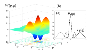
Figure 1: (a) Position and momentum distributions for an exact cat state. (b) Wigner function based on the output of the SDP.

Characteristic functions and Bochner’s theorems. – We consider physical systems of $n$ bosonic modes, associated with canonical coordinates $R=(q_{1},\dots,q_{n},p_{1},\dots,p_{n})$, of “position” and “momentum”, or some quadratures. In the center of the analysis will be quantum characteristic functions CVReviews ; Leonhardt . For $n$ modes, the quantum characteristic function $\chi:{\mathbbm{R}}^{2n}\rightarrow{\mathbbm{C}}$ is defined as

$$\chi(\xi)=\mathrm{tr}[\rho D(\xi)],\quad D(\xi)=e^{i\xi\cdot\sigma R},$$ (2)

so as the expectation value of the Weyl or displacement operator, where the matrix

$$\sigma=\left[\begin{array}[]{cc}0&\mathbbm{1}_{n}\\ -\mathbbm{1}_{n}&0\end{array}\right]$$ (3)

reflects the canonical commutation relations. This characteristic function is nothing but the Fourier transform of the familiar Wigner function $W:{\mathbbm{R}}^{2n}\rightarrow{\mathbbm{R}}$, given by

$$W(z)=\frac{1}{(2\pi)^{2n}}\int\chi(\xi)e^{-i\xi\cdot\sigma z}d\xi.$$ (4)

A key tool in the argument will be the notion of $\lambda$-positivity of a phase space function Hudson .

Definition 2 ($\lambda$-positivity)

A function $\chi:{\mathbbm{R}}^{2n}\rightarrow{\mathbbm{C}}$ is said to be $\lambda$-positive definite for $\lambda\in{\mathbbm{R}}$ if for every $m\in{\mathbbm{N}}$ and for every set of real vectors $T=(\xi_{1},\xi_{2},\dots,\xi_{m})$ the $m\times m$ matrix $M^{(\lambda)}(\chi,T)$ with entries

$$\left(M^{(\lambda)}(\chi,T)\right)_{k,l}=\chi(\xi_{k}-\xi_{l})e^{i\lambda\xi_{k}\cdot\sigma\xi_{l}/2},$$ (5)

is non-negative, so $M^{(\lambda)}(\chi,T)\geq 0$.

Eq. (2) defines the characteristic function of a given quantum state. In turn, one can ask for a classification of all functions that can be characteristic functions of a quantum state, or some probability distribution in the classical case. Such a characterization is captured in the quantum and classical Bochner’s theorems Hudson . The following assertions follow:

(i) Every characteristic function of a quantum state must be 1-positive definite.

(ii) Every characteristic function of a quantum state with a positive Wigner function must be at the same time 1-positive definite and 0-positive definite.

Measuring non-classicality. – Data are naturally taken as slices in phase space, resulting from measurements of some linear combinations of the canonical coordinates, as they would be obtained from a phase sensitive measurement such as homodyning in quantum optics. One collects data from measuring observables $u_{k}\cdot R$ for some collection of $u_{k}\in{\mathbbm{R}}^{2n}$ with $\|u_{k}\|=1$. For example, in the simplest case of one mode one could measure only $q$ and $p$ or, if the state is phase invariant, one could average over all the possible directions. With repeated measurements one can estimate the associated probability distributions $P_{k}:{\mathbbm{R}}\rightarrow{\mathbbm{R}}^{+}$, related to slices of the characteristic functions by a simple Fourier transform

$$\int P_{k}(s)e^{i\omega s}ds=\chi(\omega\sigma u_{k}).$$ (6)

Actually, in a real experiment one can build only a statistical histogram rather than a continuous probability distribution. As a consequence, measurements of values of the characteristic function must be equipped with honest error bars. An estimate of this error is given by (see Appendix)

$$\delta(\omega)=|\omega|h+{n}/{\sqrt{N}},$$ (7)

where $2h$ is the width of each bin of the histogram, $N$ is the number of measurements and $n$ is the number of standard deviations that one should consider depending on the desired level of confidence tube . This kind of measurements can be performed also in opto-mechanical systems where a particular quadrature of a mechanical oscillator can be measured a posteriori by appropriately homodyning a light mode coupled to the mechanical resonator Miao . A different idea has recently been proposed for directly pointwise measuring the characteristic function of a mechanical mode coupled to a two-level system Meystre . In both cases the method that we are going to describe can be easily applied. Restricted measurements also arise in the context of bright beams Leuchs , where Mach-Zehnder interferometers have to replace homodyning in the absence of the possibility of having a strong local oscillator. In the study of states of macroscopic atomic ensembles Mac similar issues arise.

Bounds to the non-classicality from convex optimization. – We assume that we estimate the values of the characteristic function $\chi(\bar{\xi}_{j})\simeq c_{j}$ for a given set of points $\bar{\xi}_{j}$, $j=1,\dots,p$, within a given error $\delta_{j}\geq 0$ tube , so that for all $j$

$$|\chi(\bar{\xi}_{j})-c_{j}|\leq\delta_{j}.$$ (8)

Now pick a set of suitable test vectors $T=(\xi_{1},\dots,\xi_{m})$, the differences $\xi_{j}-\xi_{k}$ of which at least contain the data points $\bar{\xi}_{1},\dots,\bar{\xi}_{p}$. Based on this, we define the following convex optimization problem as a minimization over $\chi$, $x$,

$$\mathrm{minimize} x,$$ (9)

$$\mathrm{such\,\,that} |\text{Re}(\chi(\bar{\xi}_{j}))-\text{Re}(c_{j})|\leq\delta_{j},\,j=1,\dots,p,$$ (10)

$$|\text{Im}(\chi(\bar{\xi}_{j}))-\text{Im}(c_{j})|\leq\delta_{j},\,j=1,\dots,p,$$ (11)

$$M^{(0)}(\chi,T)+x\,m\mathbbm{1}\geq 0,$$ (12)

$$M^{(1)}(\chi,T)\geq 0,$$ (13)

where $M^{(0)}(\chi,T)$ and $M^{(1)}(\chi,T)$ are the Hermitian matrices (5) associated with the $\lambda$-positivity, based on the test points $\xi_{1},\dots,\xi_{m}$ as being specified in Def. 2. The minimization is in principle performed over all functions $\chi:{\mathbbm{R}}^{2n}\rightarrow{\mathbbm{C}}$ such that $\chi(-\xi)=\chi(\xi)^{*}$, where $\chi(\bar{\xi}_{l})$ is constrained by the data and $M^{(0/1)}(\chi,T)$ depend on the test points. Since we take only a finite number of points of $\chi$, yet, the above problem gives rise to a semi-definite problem (SDP) Convex . This can be efficiently solved with standard numerical algorithms. What is more, by means of the notion of Lagrange duality, one readily gives analytical certifiable bounds to the optimal objective value: Every solution for the dual problem will give a proven lower bound to the primal problem Convex , and hence a lower bound to the measure of non-classicality itself. The entire procedure hence amounts to an arbitrarily tight convex relaxation of the Bochner constraints. We can now formulate the main result: Eq. (9) gives rise to a lower bound for the non-classicality: Given the data (and errors), one can find good and robust bounds to the smallest non-classicality that is consistent with the data.

Theorem 3 (Estimating non-classicality)

The output $x^{\prime}$ of Eq. (9) is a lower bound for the non-classicality, $\eta(\rho)\geq x^{\prime}$.

The proof proceeds by constructing a witness operator

$$F=\frac{1}{m}\sum_{k,l=1}^{m}v^{*}_{k}v_{l}D(\xi_{k}-\xi_{l}),$$ (14)

where $\xi_{1},\dots,\xi_{m}\in{\mathbbm{R}}^{2n}$ are the test vectors from Bochner’s theorem used in the SDP and $v$ is the normalized eigenvector associated with the minimum eigenvalue of $M^{(0)}(\chi^{\prime},T)$, where $\chi^{\prime}$ is the optimal solution for $\chi$. For a given state $\rho$, this operator $F$ has the following properties:

1. $F=F^{\dagger}$,

2. $|\text{tr}{(F\omega)}|\leq 1$ for all quantum states $\omega$.

3. $\text{tr}{(F\omega)}\geq 0$ for all quantum states $\omega\in\mathcal{C}$.

4. If $x^{\prime}\geq 0$ is the optimal solution, then $\text{tr}{(F\rho)}\leq-x^{\prime}$.

This can be seen as follows: 1. follows directly from construction, noting that $D(\xi)=D(-\xi)^{\dagger}$ for $\xi\in{\mathbbm{R}}^{2n}$. Property 2. follows from $|\text{tr}(D(\xi)\omega)|=|\chi(\xi)|\leq 1$, valid for every characteristic function, from which we find

$$|\text{tr}{(F\omega)}|\leq\frac{1}{m}\sum_{k,l=1}^{m}|v_{k}||v_{l}|=\frac{1}{m}\left(\sum_{l=1}^{m}|v_{l}|\right)^{2}\leq 1,$$

where we have used that for every normalized vector $\sum_{l=1}^{m}|v_{l}|\leq m^{1/2}$, as can easily be seen by solving a quadratic problem. To show 3., we can exploit the property of the characteristic function of $\omega$ of being 0-positive definite. This implies that

$$\text{tr}{(F\omega)}=\frac{1}{m}\sum_{k,l=1}^{m}v^{*}_{k}v_{l}\left(M^{(0)}(\tilde{\chi},T)\right)_{k,l}\geq 0,$$ (15)

where $M^{(0)}(\tilde{\chi},T)$ is the Bochner matrix associated with the characteristic function $\tilde{\chi}$ of $\omega$. Finally, 4.  originates from the structure of the SDP as a convex optimization problem. For optimal solutions $x^{\prime}$ and $\chi^{\prime}$, the constraint (12) implies that the minimum eigenvalue of $M^{(0)}(\chi^{\prime},T)$ is equal to $-x^{\prime}m$. Then $\text{tr}{(F\rho)}\leq\sum_{k,l=1}^{m}v^{*}_{k}v_{l}M_{k,l}^{(0)}(\chi^{\prime},T)/m=-x^{\prime}$ .

The four properties suggest that $F$ is actually a witness observable able to distinguish a subset of non-classical states from the convex set of classical states. Formally, from the variational definition of the trace norm, we have

$$\eta(\rho)=\min_{\omega\in\mathcal{C}}\|\rho-\omega\|_{1}\geq\min_{\omega\in\mathcal{C}}\text{tr}(\omega F)-\text{tr}{(F\rho)}\geq x^{\prime},$$ (16)

which is the lower bound to be shown.

An example: Schrödinger cat state. – As an example we consider a quantum superposition of two coherent states, so $|\psi\rangle\sim(|\alpha\rangle+|-\alpha\rangle)$ with $\alpha=1.77$. We assume to measure only the probability distributions of position and momentum (Fig. 1.a): $P_{1}(q)=|\langle q|\psi\rangle|^{2}$ and $P_{2}(p)=|\langle p|\psi\rangle|^{2}$, that is the data is collected from a mere pair of canonical operators. This amount of information is of course not sufficient for tomographically reconstructing the state since it corresponds to just two orthogonal slices of the characteristic function.

In order to define the SDP we consider a $25\times 25$ square lattice centered at the origin of the domain of the characteristic function and we optimize over the values of $\chi$ at the lattice points. Position and momentum measurements can be used to define constraints (10-11) for only two slices of the lattice and we assume an error of $\delta_{j}=10^{-3}$ for each point. We generate $100$ random test vectors and we construct the associated $\lambda-$positivity constraints (12-13). The output of the SDP is $x^{\prime}\simeq 0.05>0$ which is a certified lower bound for the non-classicality of the state.

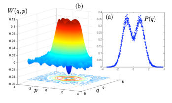
Figure 2: (a) Raw measured quadrature distribution from the experiment without any correction. (b) Related Wigner function based on the output of the SDP.

Experimentally detecting non-classicality. – Finally, to certify the functioning of the idea in a quantum optical context, we apply our method to experimental data. We consider data from a heralded single-photon source based on parametric down-conversion (cf. Ref. Polzik2 ). Here, one of the two down-converted photons is detected and heralds the presence of the other photon. The heralded single photon is sampled $180,000$ times by homodyne measurements at phase-randomized quadratures (Fig. 2.a). Instead of using these data in tomography we will use the same data to directly extract a certified lower bound to the non-classicality of the state. We will show that the most classical state consistent with those data has a negative Wigner function (Fig. 2.a) which is close to the one reconstructed with a maximum likelihood method in Ref. Polzik2 . This strengthens the finding of a negative Wigner function, as we hence directly certify it as a worst case bound including error bars. Data correspond to phase randomized measurements meaning that we can use the same probability distribution for every phase space direction, the phase being not available in this experiment. Since our non-classicality measure is convex, averaging over phase space directions is an operation which can only decrease the negativity of the state. This means that a lower bound to the non-classicality of the phase randomized state will be valid for the original state.

In order to apply our algorithm we use the measured data to constrain all the points of the characteristic function on a $37\times 37$ lattice. Error bars are estimated using Eq. (7) with $n=5$ standard deviations. This means that the probability that all the points of the lattice lie inside the error bars is larger than $99.9\%$. The lower bound for the non-classicality coming out from the SDP ($200$ random test vectors have been used) is larger than zero $x^{\prime}\simeq 0.0028$, meaning that the Wigner function of the state cannot be a positive probability distribution. Indeed, the Wigner function reconstructed from the optimal solution of the SDP (Fig. 2.b) is clearly negative even if we asked for the most positive one consistent with measured data.

Extensions of this approach. – Needless to say, this approach can be extended in several ways. Indeed, the method can readily be generalized to produce lower bounds for entanglement measures Entanglement in the multi-mode setting. Also, this idea can be applied to the situation when not slices are measured, but points in phase space, such as when using a detector-atom that is simultaneously coupled to a cantilever Meystre . It would also constitute an interesting perspective to see how the present ideas can be used to certify deviations from stabilizer states for spin systems, being those states with a positive discrete Wigner function Gross .

Summary. – We have introduced a method to directly measure the non-classicality of quantum mechanical modes, requiring less information than tomographic knowledge, but at the same time in a certified fashion. In this way, these ideas are further advocating the paradigm of “learning much from little”—getting much certified information from few measurements—complementing methods of witnessing entanglement Entanglement ; Witness , recent ideas of compressed sensing Compressed or matrix-product based MPS approaches to quantum state tomography, detector tomography Detector , or the direct estimation of Markovianity Markovian of a continuous process. It is the hope that this paper further stimulates work in the context of this paradigm.

Acknowledgments. – This work has been supported by the EU (MINOS, COMPAS, QESSENCE), and the EURYI.

I Supplementary information (EPAPS)

In this appendix, we add a discussion on measurement errors not essential for the main text. We assume data to be organized in histograms made of bins of width $2h$ centered at points $s_{j}=2hj$. The normalized height of the $j$-th bin is

$$P_{k}^{j}=\int_{s_{j}-h}^{s_{j}+h}P_{k}(s)ds+w_{j},$$ (17)

where $\{w_{i}\}$ are random variables with zero average associated to the statistical error. In a standard homodyne detection, $\{w_{j}\}$ have Poissonian variances equal to $\langle w_{j}w_{l}\rangle=\delta_{j,l}\int_{s_{j}-h}^{s_{j}+h}P_{k}(s)ds/N$, where $N$ is the total number of measurements. The simplest approximation for the value of the characteristic function defined in Eq. (6) is

$$\chi^{a}(\omega\sigma u_{k})=\sum_{j}P_{k}^{j}e^{i\omega s_{j}}.$$ (18)

The error will be the sum of two terms

$$\chi(\omega\sigma u_{k})-\chi^{a}(\omega\sigma u_{k})=\Delta+\tilde{w}.$$ (19)

The first term is the error due to the finite resolution of the histogram, which is bounded by $|\Delta|\leq h|\omega|$, while $\tilde{w}=\sum_{j}w_{j}e^{i\omega s_{j}}$ is the random statistical error. This error could be estimated and possibly reduced by using bootstrapping or maximum likelihood algorithms. For our purposes, we simply calculate the standard deviation of the random variable $\tilde{w}$, which is given by $({\langle|\tilde{w}|^{2}\rangle})^{1/2}=1/\sqrt{N}$. Now, for the central limit theorem $\tilde{w}$ can be approximated by a Gaussian distribution, meaning that the probability that the following tube constraint is violated is exponentially suppressed in the number of considered standard deviations $n$ tube ,

$$|\chi(\omega\sigma u_{k})-\chi^{a}(\omega\sigma u_{k})|\leq h|\omega|+{n}/{\sqrt{N}}.$$ (20)

References

- (1) E. P. Wigner, Phys. Rev. 40, 749 (1932); R. J. Glauber, Phys. Rev. 131, 2766 (1963).
- (2) U. Leonhardt, Measuring the quantum state of light (Cambridge University Press, 1997); W. Schleich, Quantum optics in phase space (Wiley VCH, 2000).
- (3) A. Kenfack and K. Zyczkowski, J. Opt. B 6, 396 (2004).
- (4) J. Sperling and W. Vogel, arXiv:1004.1944; Th. Richter and W. Vogel, Phys. Rev. Lett. 89, 283601 (2002); T. Kiesel et al, Phys. Rev. A 79, 022122 (2009); O. Giraud, P. A. Braun, and D. Braun, arXiv:1002.2158.
- (5) D. T. Smithey, M. Beck, M. Raymer, and A. Faridani, Phys. Rev. Lett. 70, 1244 (1993).
- (6) G. Nogues et al, Phys. Rev. A 62, 054101 (2000).
- (7) A. Ourjoumtsev, R. Tualle-Brouri, J. Laurat, and P. Grangier, Science 312, 83 (2006); A. Ourjoumtsev, A. Dantan, R. Tualle-Brouri, and P. Grangier, Phys. Rev. Lett. 98, 030502 (2007).
- (8) J. S. Neergaard-Nielsen, B. Melholt Nielsen, C. Hettich, K. Molmer, and E. S. Polzik, Phys. Rev. Lett. 97, 083604 (2006).
- (9) J. S. Neergaard-Nielsen, B. Melholt Nielsen, H. Takahashi, A. I. Vistnes, and E. S. Polzik, Opt. Exp. 15, 7940 (2007); B. Melholt Nielsen, J. S. Neergaard-Nielsen, and E. S. Polzik, Opt. Lett. 34, 3872 (2009).
- (10) S. Gigan et al, Nature 444, 67 (2006); O. Arcizet, P. -F. Cohadon, T. Briant, M. Pinard, and A. Heidmann, ibid. 444, 71 (2006); D. Kleckner and D. Bouwmeester, ibid. 444, 75 (2006); D. Kleckner et al, New J. Phys. 10, 095020 (2008), O. Romero-Isart, M. L. Juan, R. Quidant, and J. I. Cirac, New J. Phys. 12, 033015 (2010).
- (11) C. D. Cushen and R. L. Hudson, J. Appl. Prob. 8, 454 (1971); F. J. Narcowich, J. Math. Phys. 29, 2036 (1988); S. Bochner, Math. Ann. 108, 378 (1933).
- (12) M. Hillery, Phys. Rev. A 35, 725 (1987).
- (13) J. Eisert and M.B. Plenio, Int. J. Quant. Inf. 1, 479 (2003); S. L. Braunstein and P. van Loock, Rev. Mod. Phys. 77, 513 (2005).
- (14) Since the error follows a Gaussian distribution, the probability that the actual value of the characteristic function lies outside the error bar is never zero but it is exponentially suppressed for increasing . E.g., for one has , for one has , etc..
- (15) H. Miao et al, Phys. Rev. A 81, 012114 (2010).
- (16) S. Singh and P. Meystre, Phys. Rev. A 81, 041804(R) (2010).
- (17) Ch. Silberhorn et al, Phys. Rev. Lett. 86, 4267 (2001).
- (18) T. Fernholz et al, Phys. Rev. Lett. 101, 073601 (2008); B. Brask, I. Rigas, E. S. Polzik, U. L. Andersen, and A. S. Sorensen, arXiv:1004.0083.
- (19) S. Boyd and L. Vandenberghe, Convex optimization (Cambridge University Press, Cambridge, 2004).
- (20) J. Eisert, F. G. S. L. Brandão, and K. M. R. Audenaert, New J. Phys. 8, 46 (2007); O. Gühne, M. Reimpell, and R. F. Werner, Phys. Rev. Lett. 98, 110502 (2007); K. M. R. Audenaert and M. B. Plenio, New J. Phys. 8, 266 (2006).
- (21) D. Gross, J. Math. Phys. 47, 122107 (2006).
- (22) O. Gühne and G. Toth, Phys. Rep. 474, 1 (2009).
- (23) D. Gross, Y.-K. Liu, S. T. Flammia, S. Becker, and J. Eisert, arxiv:0909.3304; A. Shabani, R. L. Kosut and H. Rabitz, arXiv:0910.5498.
- (24) S. T. Flammia, D. Gross, S. D. Bartlett, and R. Somma, arXiv:1002.3839; M. Cramer and M. B. Plenio, arXiv:1002.3780.
- (25) J. S. Lundeen et al, Nature Physics 5, 27 (2009).
- (26) M. M. Wolf, J. Eisert, T. S. Cubitt, and J. I. Cirac, Phys. Rev. Lett. 101, 150402 (2008).