Star Formation Feedback and Metal Enrichment History Of The Intergalactic Medium

Abstract

Using the state-of-the-art cosmological hydrodynamic simulations of the standard cold dark matter model with star formation feedback strength normalized to match the observed star formation history of the universe at $z=0-6$, we compute the metal enrichment history of the intergalactic medium (IGM). Overall we show that galactic superwind (GSW) feedback from star formation can transport metals to the IGM and that the properties of simulated metal absorbers match current observations. The distance of influence of GSW from galaxies is typically limited to about $\leq 0.5$Mpc and within regions of overdensity $\delta\geq 10$. Most C IV and O VI absorbers are located within shocked regions of elevated temperature ($T\geq 2\times 10^{4}$K), overdensity ($\delta\geq 10$), and metallicity ($[Z/{\rm\,Z_{\odot}}]=[-2.5,-0.5]$), enclosed by double shocks propagating outward. O VI absorbers have typically higher metallicity, lower density and higher temperature than C IV absorbers. For O VI absorbers collisional ionization dominates over the entire redshift range $z=0-6$, whereas for C IV absorbers the transition occurs at moderate redshift $z\sim 3$ from collisionally dominated to photoionization dominated. We find that the observed column density distributions for C IV and O VI in the range $\log N{\rm cm}^{2}=12-15$ are reasonably reproduced by the simulations. The evolution of mass densities contained in C IV and O VI lines, $\Omega_{\rm CIV}$ and $\Omega_{\rm OVI}$, is also in good agreement with observations, which shows a near constancy at low redshifts and an exponential drop beyond redshift $z=3-4$. For both C IV and O VI   most absorbers are transient and the amount of metals probed by C IV and O VI lines of column $\log N{\rm cm}^{2}=12-15$ is only $\sim 2\%$ of total metal density at any epoch. While gravitational shocks from large-scale structure formation dominate the energy budget ($80-90\%$) for turning about 50% of IGM to the warm-hot intergalactic medium (WHIM) by $z=0$, GSW feedback shocks are energetically dominant over gravitational shocks at $z\geq 1-2$. Most of the so-called “missing metals” at $z=2-3$ are hidden in a warm-hot ($T=10^{4.5-7}$K) gaseous phase, heated up by GSW feedback shocks. Their mass distribution is broadly peaked at $\delta=1-10$ in the IGM, outside virialized halos. Approximately $(37,46,10,7)\%$ of the total metals at $z=0$ are in (stars, WHIM, X-ray gas, cold gas); the distribution stands at $(23,57,2,18)\%$ and $(14,51,4,31)\%$ at $z=2$ and $z=4$, respectively.

1 Introduction

One of the pillars of the Big Bang theory is its successful prediction of a primordial baryonic matter composition, made up of nearly one hundred percent hydrogen and helium with a trace amount of a few other light elements (e.g., Schramm & Turner, 1998; Burles et al., 2001). The metals, nucleosynthesized in stars later, are found almost everywhere in the observable IGM, ranging from the metal-rich intracluster medium (e.g., Mushotzky & Loewenstein, 1997) to moderately enriched damped Lyman systems (e.g., Pettini et al., 1997; Prochaska et al., 2003) to low metallicity Lyman alpha clouds (e.g., Schaye et al., 2003). When and where were the metals made and why are they distributed as observed? We address this fundamental question in the context of the standard cold dark matter cosmological model (Komatsu et al., 2009) using latest simulations. Our previous simulations (Cen & Ostriker, 1999a; Cen et al., 2005) provided some of the earlier attempts to address this question with measured successes. In this investigation we use substantially better simulations to provide significantly more constrained treatment of the feedback processes from star formation (SF) that drive energy and metals from supernovae into the IGM through galactic winds (e.g., Cen & Ostriker, 1999a; Aguirre et al., 2001; Theuns et al., 2002b; Adelberger et al., 2003; Springel & Hernquist, 2003).

Metal-line absorption systems in QSO spectra are the primary probes of the metal enrichment of the IGM as well as in the vicinities of galaxies (e.g., Bahcall & Spitzer, 1969). The most widely used metal lines include Mg II $\lambda\lambda$2796, 2803 doublet (e.g., Steidel & Sargent, 1992), C IV $\lambda\lambda$1548, 1550 doublet (e.g., Young et al., 1982), and O VI $\lambda\lambda$1032, 1038 doublet (e.g., Simcoe et al., 2002). We here focus on the C IV and O VI absorption lines and the global evolution of metals in the IGM. We will limit our current investigation to the observationally accessible redshift range of $z=0-6$, which in part is theoretically motivated simply because the theoretical uncertainties involving still earlier star formation are much larger. At $z=0$ the O VI line (together with C VII and O VIII lines) provide vital information on the missing baryons (e.g., Mathur et al., 2003; Tripp et al., 2008; Danforth & Shull, 2008; Nicastro et al., 2009), predicted to exist in a Warm-Hot Intergalactic Medium (WHIM) (Cen & Ostriker, 1999a; Davé et al., 2001).

For a well understood sample of QSO absorption lines, one could derive the cosmological density contained in them (e.g., Cooksey et al., 2009). Early investigations indicate that $\Omega_{\rm CIV}$ remains approximately constant in the redshift interval $z\sim 1.5-4$ (Songaila, 2001, 2005; Boksenberg et al., 2003). There have been recent efforts to extend the measurements of $\Omega_{\rm CIV}$ to $z<1.5$ (Cooksey et al., 2009) and to $z>5$ (Simcoe, 2006; Ryan-Weber et al., 2006, 2009; D’Odorico et al., 2009; Becker et al., 2009). Observations in these redshift ranges have been difficult to carry out because C IV transition moves to the UV at low redshift and to the IR band at high redshift. D’Odorico et al. (2009) find evidence of a rise in the C IV mass density for $z<2.5$. Simcoe (2006) and Ryan-Weber et al. (2006) found evidence of C IV density at $z\sim 6$ being consistent with estimations at $z\sim 2-4.5$. More recently, however, Becker et al. (2009) set upper limits for $\Omega_{\rm CIV}$ at $z\sim 5.3$ and Ryan-Weber et al. (2009) observe a decline in intergalactic C IV approaching $z=6$, which we will show are in good agreement with our simulations.

The ionization potential of O VI and the relatively high oxygen abundance are very favorable for production of O VI absorbers in the IGM (e.g., Norris et al., 1983; Chaffee et al., 1986). The rest wavelength of OVI ($1032,1037$Å) places it within the Ly-$\alpha$ forest, which makes the identifications of these lines more complicated, although being a doublet helps significantly. At $z\geq 2$, however, O VI absorption can probe the metal content of the IGM in ways complementary to what is provided by C IV lines. For example, the O VI lines can probe IGM that is hotter than that probed by the C IV lines and can reach lower densities thank to higher abundance. There are now several observational studies at redshifts $z=2-3$ that describe the properties of O VI absorbers and attempt to estimate the O VI mass density, $\Omega_{\rm OVI}$ (Carswell et al., 2002; Bergeron et al., 2002; Simcoe et al., 2004; Simcoe, 2006; Frank et al., 2008; Danforth & Shull, 2008; Tripp et al., 2008; Thom & Chen, 2008b).

At $z\sim 2-3$ there is a missing metals problem: only 10-20% of the metals produced by all stars formed earlier have been identified in stars of Lyman break galaxies (LBG), in damped Lyman alpha systems (DLAs) and ${\rm Ly}\alpha$ forest. The vast majority of the produced metals appear to be missing (e.g., Pettini, 1999). The missing metals could be in hot gaseous halos of star-forming galaxies (Pettini, 1999; Ferrara et al., 2005). We will show that most of the missing metals are in a warm-hot ($T=10^{4.5-7}$K) but diffuse IGM at $z=2-3$ of overdensities of $\sim 10$ that are outside of halos.

The outline of this paper is as follows. In §2 we detail our simulations and the procedure of normalizing the uncertain feedback processes from star formation. Results on the metal enrichment of the IGM are presented in §3. In §3.1 we give a full description of the properties of the C IV and O VI lines at $z=0-6$, followed §3.2 discussing C IV and O VI absorbers as metals reservoirs. We devote §3.3 to a general discussion of global distribution of metals, addressing several specific topics, including the metallicity of the moderate overdense regions at moderate redshift, the missing metals at $z\sim 3$. Conclusions are given in §4.

2 Simulations

2.1 The Hydrocode

Numerical methods of the cosmological hydrodynamic code and input physical ingredients have been described in detail in an earlier paper (Cen et al., 2005). The simulation integrates five sets of equations simultaneously: the Euler equations for gas dynamics in comoving coordinates, time dependent rate equations for hydrogen and helium species, the Newtonian equations of motion for dynamics of collisionless (dark matter) particles, the Poisson equation for the gravitational potential field and the equation governing the evolution of the intergalactic ionizing radiation field, all in cosmological comoving coordinates. The gasdynamic equations are solved using a new, improved hydrodynamics code, “COSMO” (Li et al., 2008) on a uniform mesh. The rate equations are treated using sub-cycles within a hydrodynamic time step due to the much shorter ionization time-scales (i.e., the rate equations are very “stiff”). Dark matter particles are advanced in time using the standard particle-mesh (PM) with a leapfrog integrator. The Poisson equation is solved using the Fast Fourier Transform (FFT) method on the uniform mesh. The initial conditions adopted are those for Gaussian processes with the phases of the different waves being random and uncorrelated. The initial condition is generated by the COSMICS software package kindly provided by E. Bertschinger (2001).

Cooling and heating processes due to all the principal line and continuum atomic processes for a plasma of primordial composition with additional metals ejected from star formation. Compton cooling due to the microwave background radiation field and Compton cooling/heating due to the X-ray and high energy background are computed. The cooling/heating due to metals is computed using a code based on the Raymond-Smith code assuming ionization equilibrium that takes into account the presence of a time-dependent UV/X-ray radiation background, which we have included in our simulations since Cen et al. (1995) and has now been performed by other investigators (e.g., Shen et al., 2010).

We follow star formation using a well defined, Schmidt-Kennicutt-law-like prescription used by us in our previous work and similar to that of other investigators (e.g., Katz et al., 1996; Steinmetz, 1996; Gnedin & Ostriker, 1997). A stellar particle of mass $m_{*}=c_{*}m_{\rm gas}\Delta t/t_{*}$ is created (the same amount is removed from the gas mass in the cell), if the gas in a cell at any time meets the following three conditions simultaneously: (i) contracting flow, (ii) cooling time less than dynamic time, and (iii) Jeans unstable, where $\Delta t$ is the time step, $t_{*}={\rm max}(t_{\rm dyn},10^{7}$yrs), $t_{dyn}=\sqrt{3\pi/(32G\rho_{tot})}$ is the dynamical time of the cell, $m_{\rm gas}$ is the baryonic gas mass in the cell and $c_{*}=0.03$ is star formation efficiency (e.g., Krumholz & Tan, 2007). Each stellar particle is given a number of other attributes at birth, including formation time $t_{i}$, initial gas metallicity and the free-fall time in the birth cell $t_{dyn}$. The typical mass of a stellar particle in the simulation is about $10^{6}M_{\odot}$; in other words, these stellar particles are like coeval globular clusters. All variations of this commonly adopted star-formation algorithm essentially achieve the same goal: in any region where gas density exceeds the stellar density, gas is transformed to stars on a timescale longer than the local dynamical time and shorter than the Hubble time. Since these two time scales are widely separated, the effects, on the longer time scale, of changing the dimensionless numbers (here $c_{*}$) are minimal. Since nature does not provide us with examples of systems which violate this condition (systems which persist over many dynamical and cooling time scales in having more gas than stars), this commonly adopted algorithm should be adequate even though our understanding of star formation remains crude.

Stellar particles are treated dynamically as collisionless particles subsequent to their birth. Feedback from star formation, the effects of the cumulative SN explosions known as Galactic Superwinds (GSW) and metal-enriched gas, will be described in more detail in the next subsection. While the code can self-consistently compute the ionizing UV-X-ray background using sources and sinks in the simulation, here we use the Haardt & Madau (1996) spectra for all runs such that we do not introduce additional variations due to otherwise varying UV backgrounds in the different runs. However, a local optical depth approximation is adopted to crudely mimic the local shielding effects: each cubic cell is flagged with six hydrogen “optical depths” on the six faces, each equal to the product of neutral hydrogen density, hydrogen ionization cross section and scale height, and the appropriate mean from the six values is then calculated; analogous ones are computed for neutral helium and singly-ionized helium. In computing the local ionization and cooling/heating balance for each cell, self-shielding is taken into account to attenuate the external HM ionizing radiation field. Both these two shielding effects are essential in order to obtain self-consistent radiation background evolution and neutral hydrogen evolution.

Table 1: Simulations

Run	Box (Mpc/h)	Res (kpc/h)	DM (${\rm\,M_{\odot}}$)	$e_{GSW}$
N	50	24	$1.1\times 10^{7}$	$0$
L	50	24	$1.1\times 10^{7}$	$3\times 10^{-6}$
M	50	24	$1.1\times 10^{7}$	$7\times 10^{-6}$
H	50	24	$1.1\times 10^{7}$	$1\times 10^{-5}$
MR	50	48	$8.8\times 10^{7}$	$7\times 10^{-6}$

Table 2: The first gives a letter label for each run. The second, third and fourth columns give the comoving box size, comoving spatial resolution and dark matter particle mass. The last column indicates the GSW strength.

2.2 Cosmological and Physical Parameters of the Simulations

We have run a set of four new simulations of a WMAP5-normalized (Komatsu et al., 2009) cold dark matter model with a cosmological constant: $\Omega_{M}=0.28$, $\Omega_{b}=0.046$, $\Omega_{\Lambda}=0.72$, $\sigma_{8}=0.82$, $H_{0}=100h{\rm kms}^{-1}{\rm Mpc}^{-1}=70{\rm km}s^{-1}{\rm Mpc}^{-1}$ and $n=0.96$. The adopted box size is $50$Mpc/h comoving and with $2048^{3}$ cells of size $24$kpc/h comoving; the dark matter particle mass and mean baryonic mass in a cell are equal to $1.1\times 10^{7}{\rm\,M_{\odot}}$ and $2.6\times 10^{5}{\rm\,M_{\odot}}$, respectively. Some of the key parameters for the four simulations are summarized in Table 1. The only difference among the four main runs is the strength of the GSW feedback: (N) no GSW, (L) low GSW feedback, (M) moderate GSW feedback and (H) high GSW feedback. In the next subsection we will determine which feedback strength produces the star formation rate history that matches observations. We run an additional lower resolution simulation with $1024$ cells a side, each of size $48$kpc/h (run “MR”) to test convergence of results. When computing results using run “MR”, we multiply the metallicity of each cell in run “MR” by a constant factor such that its mean metallicity at any epoch match that of run “M”. We obtain an additional set of results by changing the amplitude of the UV background, run “M2”, where it is reduced to one half of that in “M”.

2.3 Mechanical Feedback from Star Formation

It is well known that without impeding processes to counter the cooling and subsequent condensation of baryons, the stellar mass in the universe would be overproduced – the “overcooling” problem (e.g., White & Frenk, 1991; Cole, 1991; Blanchard et al., 1992). Feedback from star formation is believed to play the essential role to prevent gas from overcooling. The key question is: Where does the feedback from SF throttle gas cooling and condensation?

We consider three independent lines of evidence to address this question. First, while metals from supernovae ejecta can be accelerated to velocities exceeding the escape velocity, the whole interstellar gas is very difficult to be blown away, even in starburst galaxies, based on simulations (e.g., Mac Low & Ferrara, 1999), although their adopted feedback strength may be on the low side. Second, observed normal galaxies in the local universe tend to be relatively gas poor (e.g., Zhang et al., 2009). Their progeniors or their building blocks were presumably gas rich in the past when most of the star formation occurred. This implies that, once gas has collapsed, it would turn into stars on a time scale that is shorter than the Hubble time. Finally, if gas were able to collapse inside halos without hinderance, the observed soft X-ray background would be overproduced by more than an order of magnitude (Pen, 1999; Wu et al., 2001). These three lines of evidence together suggest that feedback from star formation likely exerts its effect outside normal stellar disks, probably in regions that are tens to hundreds of kiloparsecs from halo centers, before too much gas has either been collected inside the virial radius or cooled and condensed onto the disk.

It is currently difficult to fully model GSW in a cosmological simulation, although significant progress has been made to provide a better treatment of the multi-phase interstellar medium (e.g., Yepes et al., 1997; Springel & Hernquist, 2003). It is likely that a combination of both high resolution and detailed multi-phase medium treatment (perhaps with the inclusion of magnetic fields and cosmic rays) is a requisite for reproducing observations.

Here we do not attempt to model the causes and generation of GSW, but, instead, to simply assume an input level of mass, energy and metals, and carefully compute the consequences of GSW on the surrounding medium and on subsequent galaxy formation. Our simulations have a resolution of $24$kpc/h comoving (see Table 1), which may provide an adequate resolution for this purpose, given the aforementioned lines of evidence that feedback from star formation likely exerts most of its effects in regions on scales larger than tens of kiloparsecs. In our simulations, GSW energy and ejected metals are distributed into 27 local gas cells centered at the stellar particle in question, weighted by the specific volume of each cell (Cen et al., 2005). The temporal release of the feedback at time $t$ has the following form, all being proportional to the local star formation rate: $f(t,t_{i},t_{dyn})$ $\equiv(1/t_{dyn})[(t-t_{i})/t_{dyn}]$ $\exp[-(t-t_{i})/t_{dyn}]$. Within a time step $dt$, the released GSW energy and mass to the IGM from stars are $e_{GSW}f(t,t_{i},t_{dyn})m_{*}c^{2}dt$ and $e_{mass}f(t,t_{i},t_{dyn})m_{*}dt$, respectively. We fix $e_{mass}=0.25$, i.e., 25% of the stellar mass is recycled with the ejecta metallicity of $5{\rm\,Z_{\odot}}$. Metals, collectively having the observed solar abundance pattern, are followed as a separate hydro variable (analogous to the total gas density or nuetral hydrogen, HeI density, HeII density) with the same hydrocode. We do not introduce any additional “diffusion” process for the metals. We note that cooling process is never turned off, before or after the deposition of thermal energy, and hydrodynamic coupling between ejected baryons and surrounding gas is not turned off either, a departure from some of the previous simulations (e.g., Theuns et al., 2002a; Aguirre et al., 2005; Oppenheimer & Davé, 2006; Dalla Vecchia & Schaye, 2008; Shen et al., 2010). This is physically made possible in part due to a deposition of energy at scales that are comparable or larger than the Sedov radius in our current simulations, thanks to our limited spatial resolution.

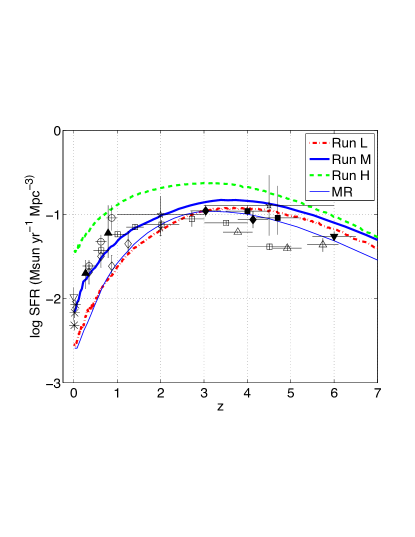
Figure 1: Star formation rate density as a function of redshift for three models with differing feedback coefficients $e_{GSW}=7\times 10^{-6}$ (run “M”, thick solid curve), $e_{GSW}=1\times 10^{-5}$ (run “H”, dot-dashed curve), $e_{GSW}=3\times 10^{-6}$ (run “L”, dashed curve), and run “M2” (thin solid curve), compared with observational data taken from (from low to high redshift): Heavens et al. (2004, 3 asterisks at $z\sim 0$), Nakamura et al. (2004, open inverted triangle at $z=0$), Lilly et al. (1996, open circles), Norman et al. (2004, filled triangles), Cowie et al. (1999, open diamonds), Gabasch et al. (2004, open squares), Reddy et al. (2005, cross at $z=2$), Barger et al. (2000, open stars at $z=2$ and 4.5), Steidel et al. (1999, filled diamonds at $z=3,4$), Ouchi et al. (2004, filled squares at $z=4,4.7$), Giavalisco et al. (2004, open triangles at $z=3-6$), and Bouwens et al. (2005, filled inverted triangle at $z=6$). The data are converted to the values with the Chabrier IMF and common values are assumed for dust extinction for the UV data.

The GSW strength is therefore controlled by one single adjustable parameter, $e_{GSW}$. We normalize $e_{GSW}$ by the requirement that the computed star formation rate (SFR) history matches, as closely as possible, the observations over the redshift range $z=0$ to $z=6$ where comparisons can be made. Figure 1 shows the SFR history for the three runs with non-zero $e_{GSW}$, (L,M,H). What is immediately evident is that the mechanical feedback strength from star formation has a dramatic effect on the overall SFR history, especially at low redshift ($z\leq 3$). At the resolution of the simulation, run “M” provides the best and excellent match to observations, where run “L” and “H”, respectively, over- and under-estimate the SFR at $z<2$. At the time of this writing we prefer to avoid introducing additional ad hoc physics to remedy this and are instead content with the ballpark agreement at $z>3$ between simulations and observations, given the large uncertainties in the observational data as evidenced by the large dispersion among different observations. At redshift zero we find that the stellar densities in the three models (L,M,H) are $\Omega_{*}=(0.011,0.0048,0.0030)$, which should be compared to the observed value of $\Omega_{*,obs}=0.0041\pm 0.0006$ (Cole et al., 2001). Our experiments indicate that, had we set $e_{GSW}=0$, the amount of stellar density $\Omega_{*}$ at $z=0$ would exceed $0.015$, in serious disagreement with observations. In this respect model “M” also agrees better with observations. Our findings are in agreement with Springel & Hernquist (2003) and Oppenheimer & Davé (2006) in that star formation rate history depends sensitively on the stellar feedback, but in disagreement with Shen et al. (2010) who find otherwise. All the subsequent results presented are based on run “M”. There is some indication that a model between “M” and “L” might provide a better match to the observations at low redshift ($z<1$) if the compilation of Hopkins et al. (2006) is used. But we note that such a model may run into a worse agreement with observations with respect to $\Omega_{*}$ at $z=0$. Currently, it is difficult to reconcile the observations of star formation rate history and $\Omega_{*}$ at $z=0$. One might appeal to an evolving IMF to provide an attractive reconcilation between the possible discrepancy (Davé, 2008). This is well beyond the scope of this investigation. In any case, a slight varied simulation, say, using an $e_{GSW}$ value between the “M” and “L” would give qualitatively comparable results. In order to test for numerical convergence we run one additional simulation, “MR”, which has the same parameters as run “M” but have half the resolution. To test the dependence of results on the extragalactic UV background we run our software pipeline through run “M” but with halving the amplitude of the UV background, called run “M2”.

Figure 2: shows the mean flux for ${\rm Ly}\alpha$ forest as a function of redshift. Our computed results are shown in asterisks. Diamonds correspond to mean transmitted flux values for each quasar in the sample of McDonald et al. (2000), and triangles correspond to the mean flux for the same observational data but binned in redshift intervals: $[3.39,4.43]$, $[2.67,3.39]$ and $[2.09,2.67]$.

It is prudent to make a self-consistency check for the value of $e_{GSW}$ that is empirically determined. The total amount of explosion kinetic energy from Type II supernovae with a Chabrier IMF translates to $e_{GSW}=6.6\times 10^{-6}$. Observations of local sturburst galaxies indicate that nearly all of the star formation produced kinetic energy (due to Type II supernovae) is used to power GSW (e.g., Heckman, 2001). Given the uncertainties on the evolution of IMF with redshift the fact that newly discovered prompt Type I supernovae contribute a comparable amount of energy compared to Type II supernovae, we argue that our adopted “best” value of $e_{GSW}=7\times 10^{-6}$ is consistent with observations and entirely within physical plausibility.

2.4 Mock Spectra and Identification of Absorption Lines

The photoionization code CLOUDY (Ferland et al., 1998) is used post-simulation to compute the abundance of C IV and O VI , adopting the UV background calculated by Haardt & Madau (1996). For ${\rm Ly}\alpha$ absorption lines we use the computed neutral hydrogen density distribution directly from the simulation that was already using the Haardt & Madau (1996) UV background in the rate equations for hydrogen and helium species. We have checked that the radiation field is consistent with observations by comparing the simulated mean transmitted flux as a function of redshift with observations. Figure 2 shows the mean transmitted ${\rm Ly}\alpha$ flux as a function of redshift from the simulation in comparison with observations. We see the ${\rm Ly}\alpha$ forest produced in the LCDM model using the adopted UV background provides an adequate match to observations over most of the redshift range compared, $z=0-4$. At $z\gtrsim 4$, our results do not seem to coincide with observations. We attribute this to the UV background used: we have only considered a quasar background, while at these high redshifts the UV radiation coming from galaxies should have a significant effect on the ${\rm Ly}\alpha$ forest. Nevertheless, we do not expect this to be an issue on the metal species considered in the following sections. These correspond to much higher energies than 1 ryd that are not affected by the UV contribution from galaxies to the ionizing radiation.

We generate random synthetic absorption spectra for each of the three absorption lines by producing optical depth distribution along lines of sight parallel to one of the three axes of the simulation box, based on density, temperature and velocity distributions in the simulation (i.e., our calculations include redshift effects due to peculiar velocities and thermal broadening). The code used is similar to that used in our earlier papers (Cen et al., 1994, 2001). We identify each absorption line as a contiguous region in the flux spectrum between a down-crossing point and an up-crossing point, both at a flux equal to $0.85$. Note that flux equal to $1$ corresponds to no absorption. For each identified line we compute its equivalent width (EW), Doppler width ($b$), mean temperature ($T$), mean metallicity ($Z$) and mean gas overdensity ($\delta$), weighted by optically depth of each pixel. We do not attempt to perform Voigt profile fitting, a procedure often used to analyze observed spectra. Because of this, we tend to not generate some of the very low column lines that are purely an effect of profile fitting process. Also, precise comparison between our mock absorbers and observed ones is not possible for some quantities, such as Doppler width distributions.

3 Results

3.1 C IV $\lambda\lambda$1548, 1550 and O VI $\lambda\lambda$1032, 1038 absorption lines

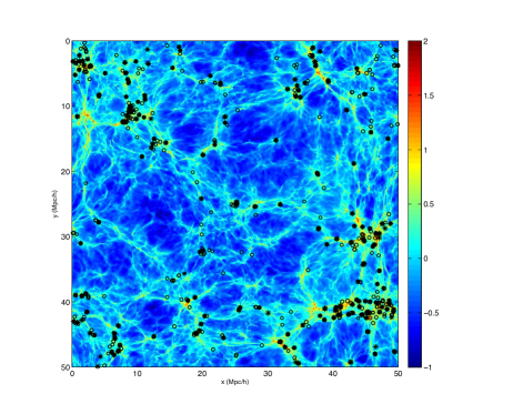
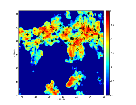
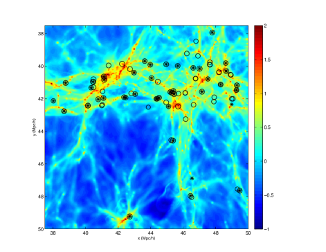
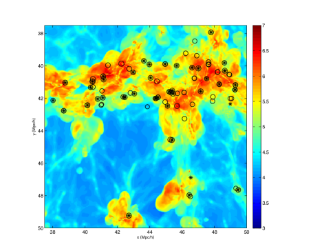
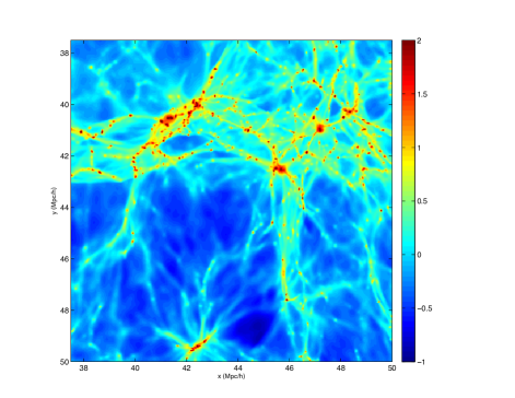
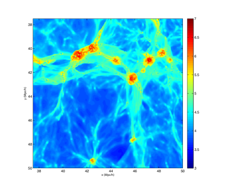
Figure 3: The top-left panel shows a slice of gas surface density in units of the mean gas surface density at $z=2.6$ of size $50\times 50$(Mpc/h)² comoving and a depth of $3.125$Mpc/h comoving. The C IV absorption lines are indicated by black asterisks, produced by sampling the slice using $8000$ random lines of sight. The O VI absorption lines are indicated by black circles. The top-right panel shows a zoom-in slice of the gas density of size $12.5\times 12.5$(Mpc/h)² comoving and a depth of $3.125$Mpc/h comoving, corresponding to the lower right corner of the top-left panel, while the bottom two panels show the corresponding gas temperature in Kelvin and gas metallicity in solar units.

We begin with a visual examination of density, temperature and metallicity distribution of IGM at $z=2.6$ and compare cases with and without star formation feedback, shown in Figure 3. Comparing the density structures in runs with (middle left panel) and without (bottom left panel) GSW we see that the effect of GSW on the overall appearance of large-scale density structure is visually non-striking and the filamentary skeleton of the large-scale density distribution remains intact. An important and visually discernible effect of GSW is to “smooth” out density concentrations in the dense (red) knots: the high density peaks ($>10^{2}$; red regions) in the run without GSW are substantially higher than those with GSW; examples include the knots at $(47,41)$Mpc/h, $(45.5,42.5)$Mpc/h and $(42,40)$Mpc/h. This effect is of course reflective of the sensitivity on GSW of the SFR history, which in turn allowed the observations of SFR history to provide a powerful constraint on GSW, as shown earlier in Figure 1.

The effect of GSW on low density (blue) regions seems small, likely because GSW do not reach there and/or become weak even if reaching there. The effect of the GSW on intermediate regions, a.k.a, filaments, is most easily seen by comparing the temperature distributions of the run with (middle right) and without (bottom right) GSW. We see that large-scale gravitational collapse induced shocks at this redshift tend to center on dense regions with a spatial extent that is not larger than about $100-300$kpc/h; these are virialization and infall shocks due to gravitational collapse of high density peaks. Some of the larger peaks are seen to be enclosed by shocks of temperature reaching or in excess of $10^{7}$ K (note that the displayed picture is inevitably subject to smoothing by projection thus the higher temperature regions have their temperatures somewhat underestimated). Galaxies form in the center of the filamentary structures where collapse of pancake structures occurs. Most of the shock heated volume from green ($10^{5}$K) to red ($10^{7}$K) are clearly caused by GSW, because they appear prominent only in the simulation with GSW. The GSW shock heated IGM seems to extend as far as $\sim 0.5$Mpc/h from galaxies. The temperature of this shock heated gas falls in the WHIM temperature range of $10^{5}-10^{7}$ K; we will discuss this more quantitatively in §3.2. Inspecting the temperature (middle right) and metal density (top right) distribution with GSW reveals that metal enriched regions, “metal bubbles”, coincide with temperature bubbles. This indicates that GSW energy and metal deposition are tightly coupled. Most of the affected regions have a size of a few hundred kiloparsecs to about one megaparsec, suggesting that this is the range of influence of GSW in transporting most of the metals to the IGM.

We now inspect visually typical physical locations of C IV and O VI absorption lines, shown as asterisks (C IV ) and circles (O VI ) in the top two rows in Figure 3. The interesting feature is that C IV and O VI absorbers tend to avoid “voids” and are almost exclusively located around filamentary structures with most of them seemingly residing in regions of an overdensity of $\sim 3-30$; however, limited resolution of our simulation prevent us from reaching firm conclusion on this at this time. For every C IV absorber that is produced, there is almost always an O VI absorber along the same line of sight. As we will see, all these paired-up C IV and O VI in fact arise from around the same regions in space. The converse is not necessarily true; a lower fraction of O VI absorbers do not have C IV counterparts within the depth of the projected slice of $3.125$Mpc/h comoving and they tend to be located in regions that are slightly further away from high density peaks than those occupied by O VI lines with associated C IV lines. The vast majority of both C IV and O VI absorbers appear to be located in regions that have been swept by feedback shocks, as evidenced by the similarly looking shock heated temperature bubbles (middle right panel of Figure 3) and metal enriched bubbles emanating from collective supernovae in star-forming galaxies (upper right panel of Figure 3). The C IV and O VI lines, either collisionally ionized or photoionized, unequivocally stem from regions that are shock heated and metal enriched by feedback from star formation; this conclusion will be confirmed quantitatively later.

The typical metallicity and temperature of the C IV and O VI absorbers appear to be around $[C/H]\sim-2$ and $T\sim 10^{4.5-5.5}$K. Typical ${\rm Ly}\alpha$ forest clouds have comparable densities but are at a significantly lower temperature, $T\sim 10^{4}$K and a lower metallicity $[C/H]\sim-3$. These properties indicate that, while most of the C IV and O VI absorption lines may have comparable overdensity compared to typical hydrogen Ly$\alpha$ forestabsorption lines ($N_{\rm HI}\sim 10^{13}-10^{15}$), the former are located in somewhat hotter regions with somewhat higher metallicity than the latter. Moreover, while many C IV and O VI lines often coincide along the same line of sight within a short distance, it will be shown that the actual gas properties of regions that produce them are significantly different.

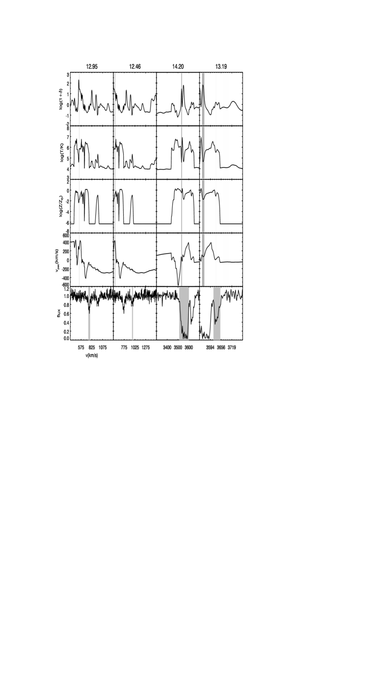
Figure 4: shows the physical properties of all C IV absorption lines (left) and O VI absorption lines (right) with column greater $10^{12}$cm^-2 along a random line of sight of length equal to the simulation boxsize of $50^{-1}$Mpc at $z=2.6$. Small regions around of all identified C IV lines along each sightline are shown in separate columns. Aside from the flux distribution shown at the bottom panel in velocity (Hubble) space, all other panels of physical variables are shown in real space. Each identified C IV absorption line in the bottom panel is indicated by a shaded region with the value of the log of its column density. The corresponding physical location that produces the line is shown by a shaded vertical line with dark shades indicating larger contributions to the column of the line.

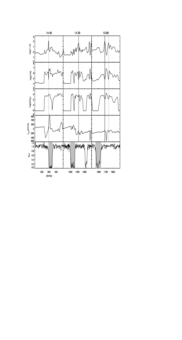
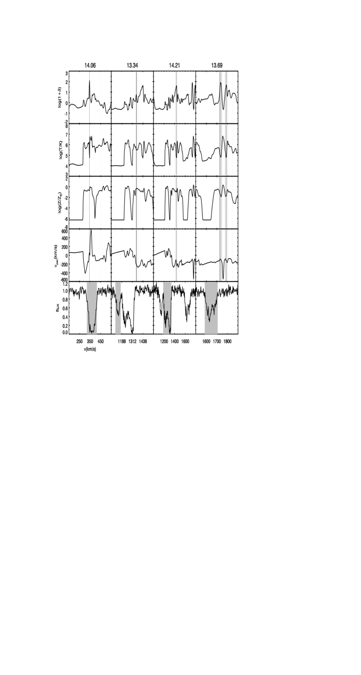
Figure 5: this is similar to Figure 4 but for another random line of sight.

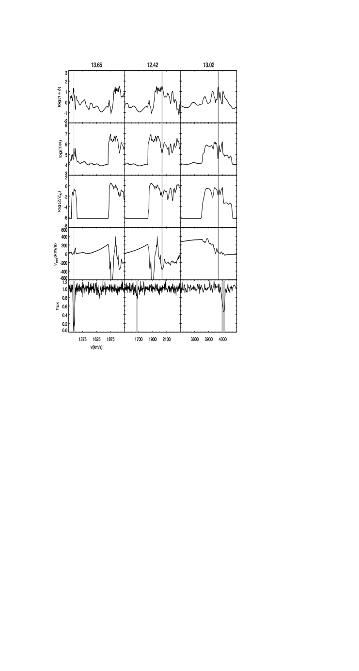
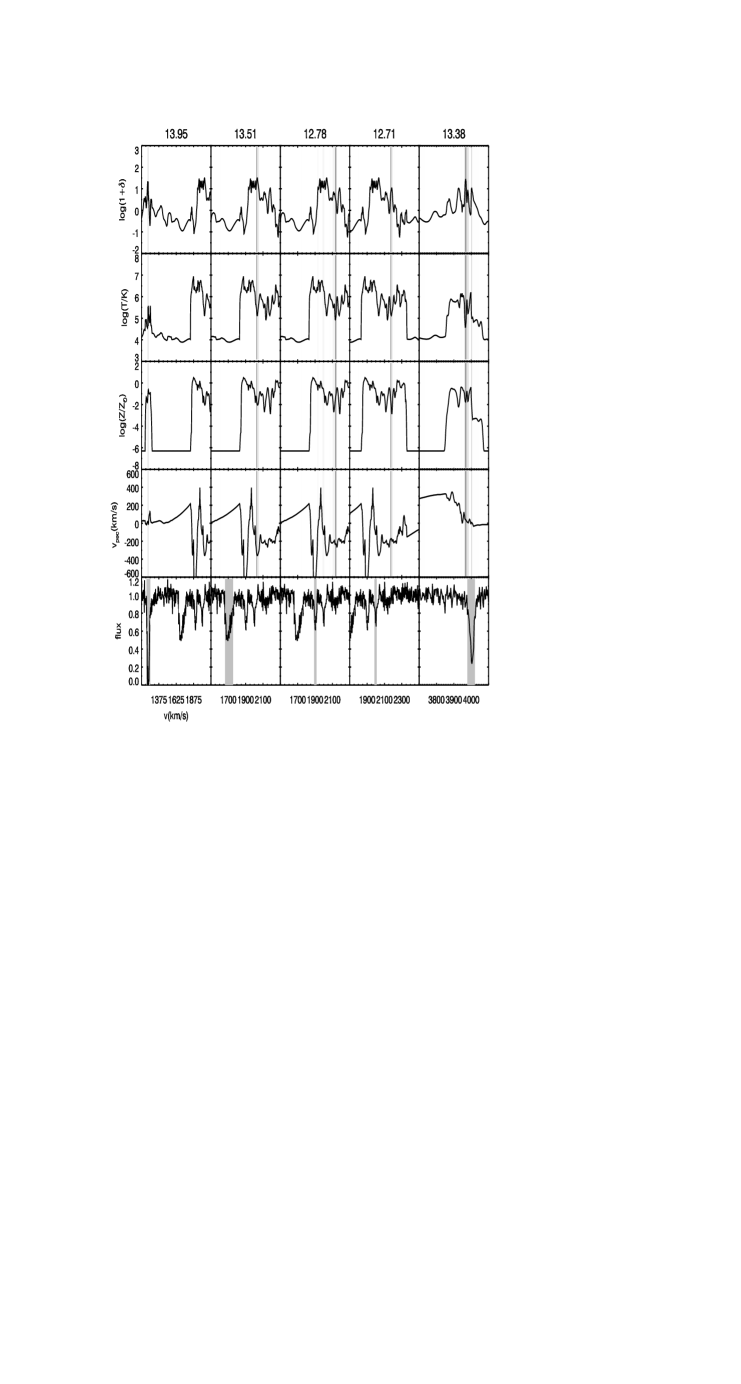
Figure 6: this is similar to Figure 4 but for another random line of sight.

Let us now examine the physical properties of C IV and O VI absorbers in greater detail. Figures 4,5,6 show three random sightlines through the simulation box. In order to better see details we have concatenated all the zoomed-in regions around identified C IV and O VI lines for each sightline to one panel, separated into columns. The left panels are for C IV lines and right for O VI lines. Several interesting properties of C IV and O VI absorbers may be gleaned. First, both C IV and O VI absorbers sit in regions with significantly elevated temperature (i.e., $>2\times 10^{4}$K) of widths of $\sim 100$km/s or larger, i.e., a few hundred physical kiloparsecs or larger, which are then connected with the general photo-ionized IGM of lower temperature of $\sim 10^{4}$K (2nd row from top in Figures 4,5,6). The density structures (top row in Figures 4,5,6) show that the densities in the regions of allevated temperatures span a wide range from $\delta\sim 0$ to $\sim 100$ and there is no clear positive correlation between density and temperature (although there is a strong anti-correlation between them near density peaks). This suggests that the elevated temperatures in these regions are not caused by gravitational compression. It is also clearly seen that at the two locations demarcating each high temperature region, there is a shock-like density jump (of a factor of a few). A closer examination of the peculiar velocity structures (2nd panel from bottom in Figures 4,5,6) shows evidence of a double shock propagating outward, with the shock fronts coincidental with the temperature and density jump.

Second, there is a tight correlation between gas temperature and gas metallicity (middle row in Figures 4,5,6) in the sense that higher temperatures have higher metallicity and each region with elevated temperature is bordered by a synchronous drop in both temperature and metallicity on two sides. This is a strong indication that the elevated temperature is caused by a double shock originating from a alaxy or small group of galaxies due to GSW, which plays the double role of both shock heating the surrounding IGM and metal-enriching it. To reiterate this important point, C IV and O VI absorbers are located in regions that have been swept through by metal-enriched feedback shocks, which are still propagating outward and “separate” the C IV and O VI absorbers from the general IGM of temperature $T\sim 10^{4}$K by about $100$km/s or more. Because of the high temperatures probed by C IV and O VI lines, they are not in general correlated with ${\rm Ly}\alpha$ lines on scales $\leq 100$km/s. The latter probe typically lower temperatures. Overall, the locations of C IV and O VI lines are closely correlated. The overall spatial extent of O VI lines, in terms of their distance from galaxies, are somewhat larger than that of C IV lines, as seen in Figure 3 and Figures 4,5,6 and will be verified by their origin being in somewhat lower density gas than C IV lines (see Figure 9 below).

Third, many C IV absorbers appear to be paired up with O VI absorbers. For brevity, our convention is that we count absorption lines from left to right in each panel. For example, the first and fourth O VI lines in the right panel can be respectively paired up with the first and third C IV lines in the left panel of Figure 4; the first, third and fourth O VI lines in the right panel can be respectively paired up with the first, second and third C IV lines in the left panel of Figure 5; the second and fifth O VI lines in the right panel can be respectively paired up with the second and third C IV lines in the left panel of Figure 6. The O VI lines that appear together with C IV lines seem to have relatively low temperature ($T\sim 10^{4.5}-10^{5}$K), probably with a significant photoionization component. Note that collisional ionization makes maximum contribution to O VI production at $T=10^{5.5}$K, whereas for C IV this happens at $T=10^{5.0}$K. Thus, it appears that relatively low-temperature O VI lines are often paired up with a C IV line, for which both photoionization and collisional ionization may be relevant. The excess of O VI lines compared to the number of C IV lines is likely due to the difference in the number of collisionally ionized cases for the two lines, given the difference in the optimal temperatures for collisional ionization for C IV and O VI lines. Note that with collisional ionization alone, the abundance of each species drops when the temperature moves away from the optimal temperature to either side (lower or higher) - a factor of $\sim 10$ drop when temperature differs from the optical temperature by a factor of two. Roughly speaking, while the probability of an associated O VI line for a given C IV line is close to unity, the probability of an associated C IV line for a given O VI is somewhat lower. A more detailed study of this issue will be performed in sections to come.

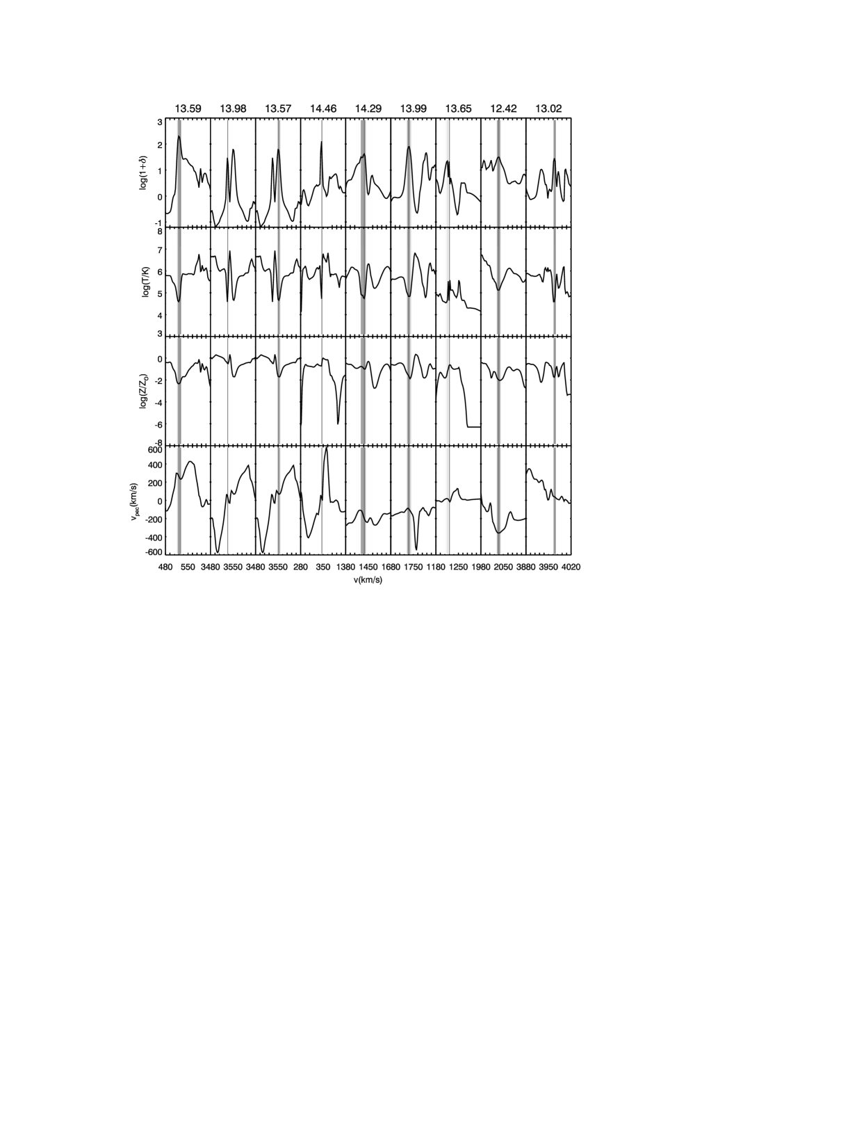
Figure 7: shows a close-up view of the region around each C IV line in real space, where the physical size along the line of sight has been translated to velocity using $\Delta v=H(z)\Delta x$. Each tickmark is $10$ km/s.

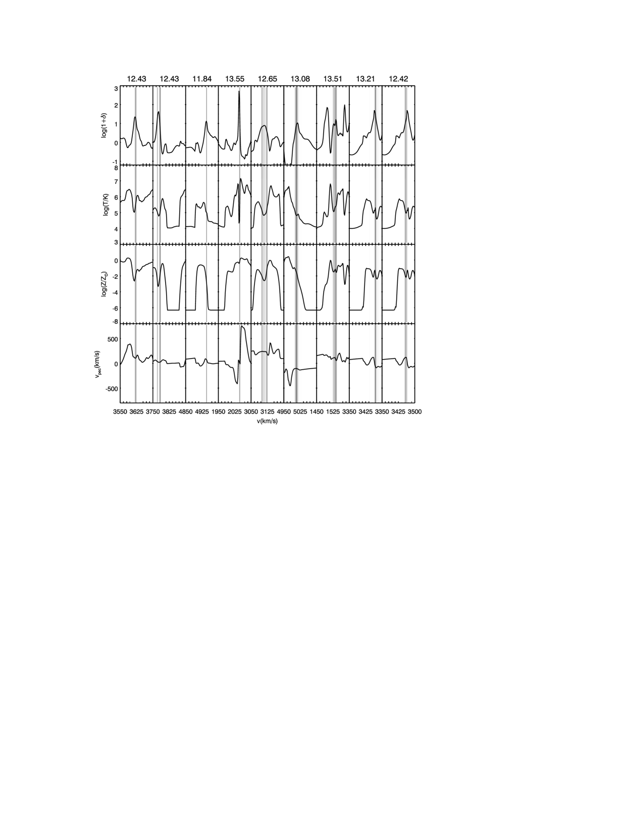
Figure 8: shows a close-up view of the region around each O VI line in real space, where the physical size along the line of sight has been translated to velocity using $\Delta v=H(z)\Delta x$. Each tickmark is $10$ km/s.

Finally, in Figure 7 we show a close-up view of several randomly chosen C IV lines. It is clear that the regions contributing to a C IV line tend to be centered or nearly centered on a local density peak along the line of sight, which almost always corresponds to a trough in temperature. It is also evident that the spatial extent of the C IV producing region is limited to about up to $10$ km/s, corresponding to about comoving $100$kpc/h, with some regions much narrower than that. As a consequence, even though the velocity gradients in the intermediate vicinities (i.e., the whole surrounding region of elevated temperature) of C IV -producing regions are often large (with $dv/dr\sim$ a few $100{\rm\,km/s}$ per comoving Mpc), the velocity gradients in the actual C IV -producing regions is smaller, which, in conjunction with the narrowness of the C IV -producing region, limits the velocity contribution to the Doppler width, as will be shown quantitatively later. Physically, this tells us that each C IV absorber tends to arise primarily from a narrow region in real space that have previously thermalized through feedback shocks, have cooled and are presently relatively quiescent. There does not appear to be a visible correlation between the LOS size of C IV lines and the column density; some of the high column C IV lines shown (the second and fourth panel from left) appear to come from very narrow regions of size $\ll 100$kpc comoving which appear to have very steep velocity gradients (for example, the fourth from left line with log of column equal 14.46). The C IV lines are mostly intergalactic in origin, not from inside galaxies.

We next examine several randomly chosen O VI lines in close-up shown in Figure 8 and make detailed comparisons of the physical properties with C IV lines, when possible. We note three points. First, in Figures 4,5,6 we noted that most C IV lines ($\geq 10^{13.5}$) have associated O VI lines that have comparable column densities. This indicates that both C IV and O VI lines of relatively high column ($\geq 10^{13.5}$) tend to arise in regions in or near density peaks and temperature troughs. Second, a typical O VI line tends to have a lower column density due to a steeper column density distribution of O VI lines (see Figure 15 below). Third, O VI lines often lie in regions that are offset from density peaks by $\sim 10-100$ km/s, and often these density peaks do not have corresponding temperature troughs. This is clear evidence that many, lower column O VI lines arise from regions that are not physically bound and instead they are mostly transient, stemming from density and temperature fluctuations in shock heated regions in the neighborhood of galaxies. It may be that the steeper column density distribution for O VI lines has its origin in the abundance of these more transient structures. The low density, shock heated regions may have temperatures that are too high to produce equally abundant C IV lines in conjunction with a lower abundance of carbon than oxygen.

Figure 9: Left panel shows the distribution of gas overdensity of regions that produce the CIV absorption lines at six different redshifts, $z=0,0.5,1.5,2.6,4,5$, separately for three subsets of lines of column density in the range of $\log$N${}_{C~{}IV\ }{\rm cm}^{2}$=[12,13],[13,14],[14,15], respectively. Right panel shows the counterpart for O VI absorption lines.

We now quantify the properties of C IV and O VI absorbers by different projections through the multi-dimensional parameter space spanned by several fundamental physical variables. Figure 9 shows the distribution of gas overdensity for C IV (left) and O VI absorbers (right) at six different redshifts, $z=(0,0.5,1.5,2.6,4,5)$. First, a comparison of the three histograms for three subsets of C IV and O VI absorbers in each panel indicates that higher column C IV and O VI absorbers are produced, on average, by higher density gas. Second, there is a clear trend that C IV absorbers trace increasingly more overdense regions with decreasing redshift. For example, while the location of the vast majority of C IV absorbers with $\log($N${}_{C~{}IV\ }{\rm cm}^{2})=[12,13]$ appears to be outside virialized regions (i.e., overdensity less than about $100$) at $z>2.6$, a significant fraction of them reside in virialized regions at $z<1.5$; the same is true for higher column O VI absorbers. A comparison to O VI absorbers reveals a striking contrast: the vast majority of O VI absorbers with $\log($N${}_{C~{}IV\ }{\rm cm}^{2})\leq 14$ are located outside virialized regions at all redshifts. In addition, typical O VI lines arise from somewhat lower density regions than C IV lines. For example, for O VI absorbers of $\log($N${}_{C~{}IV\ }{\rm cm}^{2})=[12,13]$, the typical overdensity peaks at $\delta\sim 5$ for O VI absorbers versus $\sim 10$ for C IV lines at $z=2.6-5$, which jumps to $\delta\sim 10$ for O VI absorbers versus $\sim 50$ for C IV absorbers at $z=1.5$. A more quantitative analysis of the cross correlation between C IV and O VI absorption lines and galaxies will be presented in a later paper.

Figure 10: The left panel shows the distribution of gas metallicity in solar units of regions that produce the CIV absorption lines at six different redshifts, $z=0,0.5,1.5,2.6,4,5$, separately for three subsets of lines of column density in the range of $\log$N${}_{C~{}IV\ }{\rm cm}^{2}$=[12,13],[13,14],[14,15], respectively. Right panel shows the counterpart for O VI absorption lines.

Figure 10 shows the distribution of gas metallicity for C IV (left) and O VI absorbers (right) at six different redshifts, $z=(0,0.5,1.5,2.6,4,5)$. We see that C IV absorption lines arise from gas with a wide range of metallicity from [C/H]=-3 to -0.5, peaked approximately around -2.5 to -1.5 at $z>0.5$. At $z>2.6$ the distribution for O VI lines is roughly like taking the left end of each corresponding C IV distribution and squeezing the whole distribution rightward by an amount of $\sim 0.5-1.0$. So the metallicity distributions for O VI absorbers are generally cut off at a higher metallicity than those for C IV absorbers at the low end by about $0.5-1.0$ and peak at a metallicity that is higher by this factor. The situation appears to start reversing at $z=1.5$ such that at $z<0.5$ the fraction of high metallicity C IV absorbers exceeds that of O VI absorbers. What is also interesting is that the typical metallicity of C IV and O VI lines displays a non-monotonic trend at a fixed column density. For O VI absorbers, at $z=4-5$ the metallicity of O VI lines with $\log($N${}_{O~{}VI\ }{\rm cm}^{2})=[12,14]$ peaks at $[Z/{\rm\,Z_{\odot}}]=-1.5$ to $-1.0$, which moves to a lower value of $[Z/{\rm\,Z_{\odot}}]=-2.0$ to $-1.5$ at $z=2.6$, then slightly moves back up to $[Z/{\rm\,Z_{\odot}}]\sim-1.5$ at $z=(1.5,0.5,0)$. For comparison, the overall behavior for C IV lines is as follows: the metallicity of C IV lines with $\log($N${}_{C~{}IV\ }{\rm cm}^{2})=[12,14]$ peaks at $Z=-2.0$ to $-1.5$ at $z=5$, at $[Z/{\rm\,Z_{\odot}}]\sim-2$ at $z=4$, followed by a very broad distribution peaking at $Z=-2$ to $-1$ at $z=1.5$ to $z=2.6$ with a larger fraction reaching a relatively high metallicity gas with $[Z/{\rm\,Z_{\odot}}]>-1$.

The overall trend in metallicity evolution with redshift for the C IV and O VI absorbers could be understood as follows. Let us first note that the ionizing radiation background at $z=4,5$ is about ($1/3,1/30$) of that $z=2.6$, which in turn is larger than that at $z=(1.5,0.5,0)$ by a factor of $\sim(2,7,30)$. At $z=4-5$ both C IV and O VI absorbers are predominantly collisionally ionized with the temperatures peaking at $10^{5}$K and $10^{5.5}$K, respectively, as shown below in Figure 11. These regions are relatively closer to galaxies, from which metal-carrying shocks originate and have relatively high metallicities. At lower redshift $z=2.6$ larger regions around galaxies have been enriched with metals and the rise of the ionizing radiation background produces a large population of photoionized C IV and O VI lines at lower temperature and lower metallicity. Towards still lower redshift $z<1.5$, the decrease of the mean gas density in the universe demands a rise in overdensity of the O VI -bearing gas in order to produce a comparable column density, causing a shift of these regions to be closer to galaxies where both metallicity and density are higher, seen in Figure 9.

The combination of lower density (Figure 9) and higher metallicity (Figure 10) for the typical (low) column density O VI absorbers compared to C IV absorbers is reminiscent of metal-carrying shocks propagating through inhomogeneous medium, exactly the situation one would expect of the feedback shocks from galaxies entering the highly inhomogeneous IGM. Given the widespread steep density gradients (steeper than $-2$) in regions just outside the virial radius of galaxies, these shocks could not only heat up lower density regions to higher temperatures but also enrich them to higher metallicity. The feedback shocks generically propagate in a direction that has the least resistance and is roughly perpendicular to the orientation of a local filament where a galaxy sits, as seen clearly in Figure 3 and shown previously (e.g., Theuns et al., 2002b; Cen et al., 2005). While higher density regions, on average, tend to have higher metallicity (as we will show later), the dispersion is sufficiently large that the reverse and other complex situations often occur in some local regions. This appears to be what is happening here, at least for some regions that manifest in C IV and O VI lines.

Figure 11: Shows the distribution of gas temperature of regions that produce the C IV absorption lines at six different redshifts, $z=0,0.5,1.5,2.6,4,5$, separately for three subsets of lines of column density in the range of $\log$N${}_{C~{}IV\ }{\rm cm}^{2}$=[12,13],[13,14],[14,15], respectively. Right panel shows the counterpart for O VI absorption lines.

Figure 11 shows the distribution of gas temperature for C IV (left) and O VI (right) absorbers. We see that the temperatures of C IV absorbers at $z=5$ and O VI absorbers at $z=4-5$ narrowly peak at $10^{5}$K and $10^{5.5}$K, respectively, suggesting that collisional ionization makes the dominant contribution to both species and the two types of absorbers arise from different regions. The rapid drop in the amplitude of the UV radiation background beyond $z=3$ and increase in gas density with $(z+1)^{3}$ is the primary reason for diminished component of photoionized C IV and O VI absorbers at these high redshifts. At redshift $z<2.6$ the distributions for the two absorbers become progressively broader ranging from $10^{4.3}$K to $10^{5.5}$K for C IV absorbers, and from $10^{4.3}$K to $10^{6}$K for O VI absorbers. Thus, at $z<2.6$ both C IV and O VI absorbers are a mixture of photoionized and collisionally ionized ones. For both C IV and O VI lines, while the temperature distributions of O VI lines at $z<2.6$ are broad, there is no significant segregation in temperature of lines of different column densities. Recall that there is a noticeable correlation between column density and overdensity for both O VI lines and C IV lines (Figure 9). This is likely indicative of complex, inhomogeneous nature of metal enrichment process around galaxies.

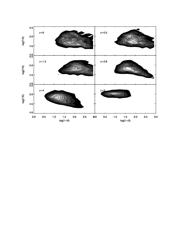
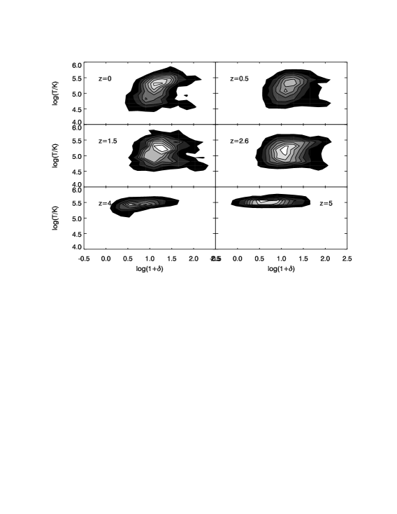
Figure 12: The left panel shows the column density-weighted distribution of C IV lines in the overdensity-temperature plane at six different redshifts, $z=0,0.5,1.5,2.6,4,5$. Right panel shows the counterpart for O VI absorption lines.

Figure 12 displays the distribution of C IV (left) and O VI (right) absorbers in the overdensity-temperature plane at redshift $z=0,0.5,1.5,3,4,5$. We again see relatively narrow peaked temperature distribution at redshift $z=4-5$ for O VI absorbers, whereas at the same redshifts the C IV absorbers have a relatively broader temperature distribution. Towards lower redshift there appears to be a multi-modal distribution in temperature for C IV absorbers, with the lower temperature peak at $T\sim 10^{4.2-4.5}$K being progressively more important with decreasing redshift and becoming dominant by $z=0$. The lower temperature peak is photoionized. At redshift $z=1.5-2.6$ a higher temperature peak at $T\sim 10^{4.5-4.8}$K is dominant, which is likely a mixture of collisional and photoionization. It is interesting to note that at $z=2.6$ the radiation background is high enough to allow for the existence of a small peak at ($\delta\geq 200$, $T=10^{4.2}$K) for C IV absorbers, clearly arising from gas that is within virialized regions. At redshift $z=0-0.5$ the peak at $T\sim 10^{4.5-4.8}$K is still prominent. But, another peak at still higher temperature of $T\sim 10^{5.0-5.2}$K emerges, which is likely dominated by collisional ionization. Overall, the composition of C IV absorbers changes from being dominated by collisional ionization at $z=4-5$, through a mixture of collisional and photoionization at $z=1.5-2.6$, to being dominated by photoionization by $z=0$. The distinct high temperature peak at $T\sim 10^{5}$K and density $\delta\sim 20$ at $z=0$ is rooted in the Warm-Hot Intergalactic Medium (WHIM; Cen & Ostriker (1999b); Davé et al. (2001); Cen & Ostriker (2006)), where the intergalactic medium has been heated up by gravitational shocks due to the formation of the large-scale structure.

A similar progression from mainly collisionally ionized to a mixture of collisional and photoionization for O VI absorbers is also seen. However, for O VI absorbers, the photoionization peak at $T\leq 10^{5}$K never dominates at any redshift. For both C IV and O VI absorbers there is no visible correlation between overdensity and temperature for O VI absorbers at all redshifts. For example, there is no evidence of these regions obeying the so-called equation of state (Hui & Gnedin, 1997) that is applicable to low redshift ${\rm Ly}\alpha$ forest clouds. This just reinforces the statement that these regions are shock heated, in a dynamical state and perhaps transient, and do not resemble photo-heated ${\rm Ly}\alpha$ forest region. We have also plotted (not shown) the distribution of C IV and O VI absorbers in the overdensity-metallicity plane and find no visible correlation between them.

Figure 13: Left panel shows the distribution of Doppler width of computed CIV absorption lines at six different redshifts, $z=0,0.5,1.5,2.6,4,5$, separately for three subsets of lines of column density in the range of $\log$N${}_{C~{}IV\ }{\rm cm}^{2}$=[12,13],[13,14],[14,15], respectively. Right panel shows the distribution of the parameter $\eta$ at four different redshifts, $z=1.5,2.6,4,5$, separately for three subsets of lines of column density in the range of $\log$N${}_{C~{}IV\ }{\rm cm}^{2}$=[12,13],[13,14],[14,15], respectively. We note that $\eta=1$ corresponds to a Doppler width that is 100% thermally broadened, whereas $\eta=0$ corresponds to a Doppler width that has no thermal contribution.

The left panel of Figure 13 shows the distribution of Doppler width of computed C IV absorption lines. The Doppler width distributions generally peak at $10-20$km/s at all redshifts. Such a Doppler width peak is consistent with thermal broadening by gas temperature $T\sim 10^{4.5}-10^{5}$K as seen Figure 11. Because of the different definition of absorption lines we use compared to Voigt profile fitting procedure for obtaining lines observationally, a direct comparison is not possible. Nonetheless, our results are consistent with the Doppler widths of the CIV absorber sample in Danforth & Shull (2008), the mean Doppler parameter at $\langle z\rangle=0.06$ is $\langle b_{C~{}IV\ }\rangle=23\pm 13$, while for our whole sample at $z=0$, the mean is $\langle b_{C~{}IV\ }\rangle 15.6\pm 7.1$ (1$\sigma$ interval). Comparisons to other samples, such as the one in Boksenberg et al. (2003), are difficult. The reason for this is that it is common in observational investigations to fit a several number of components (with a Gaussian velocty distribution each) to each absorption line. This “component” vs. “system” definition makes comparisons between our work and observations subtle at least. Our definition of an absorber by establishing a flux threshold more closely resembles the standard definition of a “system”, and in general we limit our comparisons to observational samples of “systems”. Using this method, a large number of “componentes” might be fitted to one “system”. In the sample of Boksenberg et al. (2003), this is as large as $32$ components for one given system at $z=2.438$; on average, there are $4.8$ “components” per “system” in this sample ranging between $1.6<z<4.4$.

The right panel of Figure 13 characterizes the nature of the Doppler width of computed C IV absorption lines using parameter $\eta$ $\equiv\sqrt{\frac{2kT}{m_{\rm ion}b^{2}}}$. It is indeed seen that most of the lower column density C IV absorbers with $\log($N${}_{C~{}IV\ }{\rm cm}^{2})=[12,13]$ are dominated by thermal broadening. However, for higher column C IV absorbers, there appears to be roughly equal contributions to the Doppler width from thermal broadening and bulk velocity broadening. What this suggests is that lower column C IV absorbers tend to lie in quiescent regions, whereas high column ones typically reside in regions with significant velocity structures. This was seen earlier in Figures 4, 5, 6. Once again, it is important to stress that, even though the relative contribution to the line width from velocity structure is moderate for most C IV lines, the most likely physical explanation for the C IV producing regions is that they were shock heated by sweeping feedback shocks originating from nearby galaxies, have cooled to about $10^{4.5}-10^{5}$K and perhaps somewhat compressed in the process. Most C IV lines are far from shock fronts, whose velocity structures would otherwise make the lines significantly wider. Rauch et al. (1996) suggested that the quiescence of C IV lines may be due to the adiabatic compression of gas, which would not produce large velocity gradients. We show that this explanation may be incorrect given that most of the regions producing C IV lines at $z>2$ lie outside virialized regions. Rather, the quiescence is due to a combination of two things: the thermalization of previous shocks that reduces the random velocities and velocity gradients, and the narrow range of the region in physical space that produces the C IV line, which limits the velocity difference.

Figure 14: Left panel shows the distribution of Doppler width of computed O VI absorption lines at four different redshifts, $z=1.5,2.6,4,5$, separately for three subsets of lines of column density in the range of $\log$N${}_{O~{}VI\ }{\rm cm}^{2}$=[12,13],[13,14],[14,15], respectively. Right panel shows the distribution of the parameter $\eta$ at four different redshifts, $z=1.5,2.6,4,5$, separately for three subsets of lines of column density in the range of $\log$N${}_{O~{}VI\ }{\rm cm}^{2}$=[12,13],[13,14],[14,15], respectively. We note that $\eta=1$ corresponds to a Doppler width that is 100% thermally broadened, whereas $\eta=0$ corresponds to a Doppler width that has no thermal contribution.

The left panel of Figure 14 shows the distribution of Doppler width of computed O VI absorption lines. For the OVI absorber sample of Danforth & Shull (2008), the mean Doppler parameter at $\langle z\rangle=0.06$ is $\langle b_{O~{}VI\ }\rangle=30\pm 16$, while for our whole sample at $z=0$, the mean is $\langle b_{O~{}VI\ }\rangle 22\pm 13$ (1$\sigma$ interval is quoted in both cases). In Thom & Chen (2008a), Voigt profile fitting yields a mean number of $\sim 1.4$ “components” in $27$ absorbers along 16 lines-of-sight towards QSOs, with a mean redshift of $\sim 0.25$ and a corresponding Doppler width and $1\sigma$ of $\langle b_{O~{}VI\ }\rangle=27\pm 17$. Thus, within the errorbars our results agree with both observations. A comparison with C IV lines shown Figure 13 is instructive. First, while the distributions for C IV and O VI lines of $\log$N${}_{O~{}VI\ }\,{\rm cm}^{2}$=[12,13] peak at comparable $b\sim 10{\rm\,km/s}$ at $z=1.5$ and $z=2.6$, suggesting limited velocity contribution to the widths of both lines, the distribution for O VI lines peaks at $b\sim 20{\rm\,km/s}$ at $z=4-5$, significantly higher than that of C IV lines at the same redshifts. This is indeed to be expected: the ratios of C IV and C ($f_{C~{}IV\ }$) and of O VI and O ($f_{O~{}VI\ }$) have a different dependence on density and temperature. At these densities and high temperatures, $f_{C~{}IV\ }$ increases with increasing density, whereas $f_{O~{}VI\ }$ decreases with increasing density. So If you are looking for broad lines, you will in C IV have an advantage going to high-z (where physical gas densities are higher), but not in O VI . Second, it is clear that a significant larger fraction of higher column O VI lines of $\log$N$\,{\rm cm}^{2}$=[13,15] have larger Doppler width with $b\geq 40{\rm\,km/s}$ at all redshifts than C IV lines, suggesting that there are significantly more O VI lines that C IV lines that are in dynamically hot regions, such as around shocks where velocity gradients are high. Since these dynamically hot regions likely also have higher temperatures, collisional ionization would make a larger contribution to O VI lines than C IV lines, consistent with our earlier statements. Third, let us take a close look at $\eta$ distribution for $\log($N${}_{O~{}VI\ }\,{\rm cm}^{2})$=[13,14] O VI lines and compare to that of C IV in Figure 13: for O VI lines it appears that the velocity contribution to the Doppler width is highest (i.e., lowest $\eta$) at $z=2.6$, whereas for C IV lines that occurs at $z=4$, suggesting that the fraction of C IV that are in dynamically hot regions peaks at a higher redshift than that for O VI lines. This is intriguing and likely due to a combination of several factors, including the evolution of the mixture of photoionized and collisionally ionized absorbers, evolution of metal enrichment and feedback shock strengths as a function of redshift. Potentially, useful and quantitative measures may be constructed to probe feedback processes using C IV , O VI and other lines jointly.

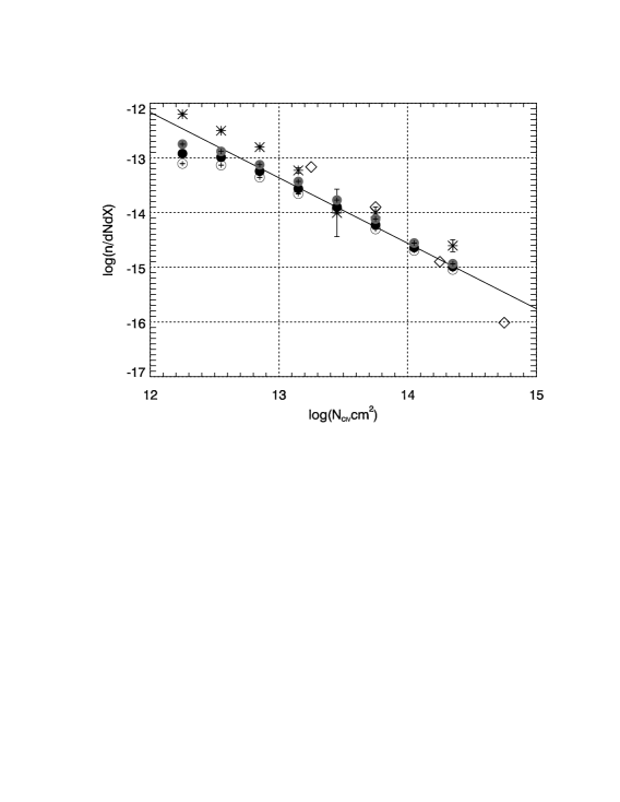
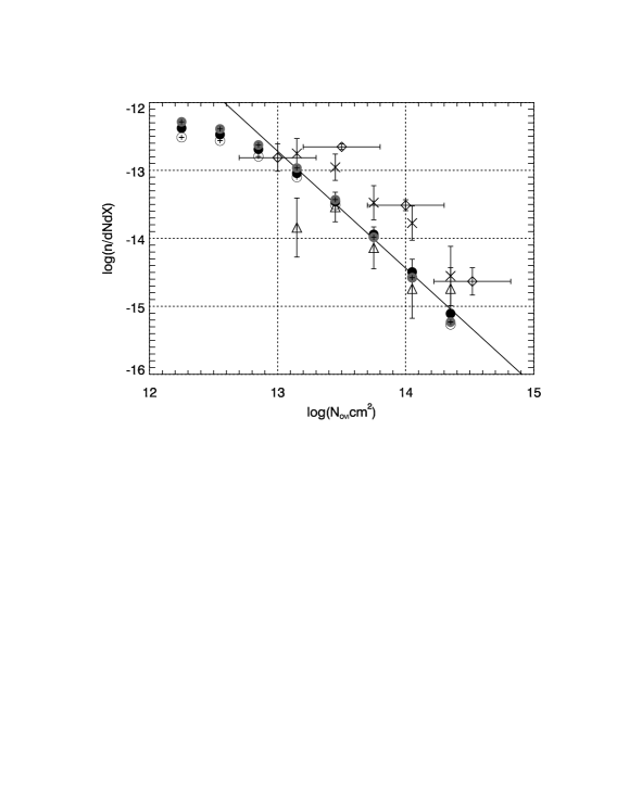
Figure 15: Left panel: the computed column density distribution for the C IV absorption line at $z=2.5$ for runs “M” (filled black circles), “MR” (open circles) and “M2” (filled grey circles). The solid line is the best power-law fit to our simulated results from run “M” performed for column densities in the range $[13,14.5]$. The slope of the fit is $-1.196\pm 0.028$. Diamonds are observational data from Songaila (2005) and Boksenberg et al. (2003) at a mean redshift of $2.7$ and $2.6$, respectively, corrected for our cosmology. Right panel: the computed column density distribution for the O VI absorption line at $z=2.5$ is shown as the solid line, which is the best power-law fit to our simulated results, with slope $-1.723\pm 0.075$. The circles have the same meaning as in the left panel. The observational data are drawn from Carswell et al. (2002) (squares), Bergeron & Herbert-Fort (2005) (diamonds), and Simcoe et al. (2002)(triangles) corrected for our cosmology.

3.2 C IV And O VI Absorbers As Baryonic Matter Reservoirs

Having gained a good understanding of the physical nature of C IV and O VI lines, we now turn to their overall column density distributions at $z=2.5$, where observational data is most accurate, shown in Figure 15. For both C IV and O VI , the results obtained from runs “M”, “’MR’ and “M2” show some small difference that is smaller than the magnitude of the difference between different observational studies and comparable to the difference between simulations and observations. This shows that our simulations are reasonably converged and not too sensitive to a factor $2$ or so variation in the strength of the UV backgrond. It is noted, however, that the convergence becomes much better for clouds with column density greater than $10^{13}$, indicating that our current simulation resolution probably still somewhat underestimates the abundance of clouds with columns smaller than that. The error bars are not visible for the simulated values because they lie within the symbols plotted. Overall, we find the agreement of the computed distributions from the simulation to the observed ones is at the level that we could have hoped for. We believe that differences may be contributable in part to cosmic variance, in part to our resolution at the lower column density (as evidenced by the noticeable flattening) and in part due to different methods of identifying clouds (flux thresholding in our case versus Voigt profile fitting in the observed results, with the latter often producing multiple components for a single physical system). Given the fact that our simulation has essentially only one free parameter ($e_{GSW}$) that has already been significantly constrained by the SFR history of the universe, it is really remarkable that we are able to match the observed column density distribution of both C IV and O VI lines to within a factor of 2-3. Since the regions probed by C IV lines and O VI lines are often physically different and to some extent reflect the different stages of the evolution of the feedback shocks, the fair agreement between our simulations and observations suggests that our treatment of the feedback process provides a good approximation to what happens in nature in terms of heating and enriching the IGM, and it is indirect but strong evidence that feedback from star formation plays the central role in enriching the IGM with its energy and metals. No additional, significantly energetic feedback from AGN seems required to account for the enrichment history of the IGM. Therefore, it is very encouraging to note that the overall picture of the process of star formation feedback may be jointly probed by C IV , O VI lines and other diagnostics. Detailed comparisons between simulations and observations in that regard would be the next logical step to further constrain theories of overall star formation in galaxies and feedback.

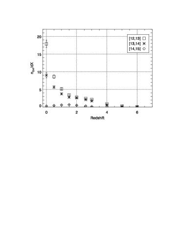
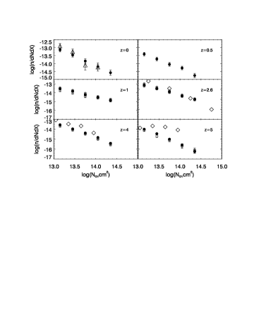
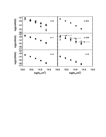
Figure 16: Top left panel: the evolution of the abundance of C IV absorbers separately for three subsets with column density in the range $\log$N${}_{C~{}IV\ }{\rm cm}^{2}$=[12,13],[13,14],[14,15], respectively. Top right panel: the same for O VI absorbers. Bottom left panel: column density distribution ($\log$f($N$)) for C IV absorbers at $z=0,0.5,1,2.6,4,5$. The results for our runs “M” (filled black circles), “MR” (open circles) and “M2” (filled grey circles) are shown. Open diamonds correspond to observations (Songaila, 2001) corrected for our adopted cosmology, except at z=2.6, when they correspond to Songaila (2005). At $z=2.6$ and $z=4$, asterisks correspond to Boksenberg et al. (2003) for $3$ and $1$ sightline respectively in a $0.5$ redshift interval around the mean redshift. At $z=0$, the observational data correspond to Danforth & Shull (2008) (triangles) and Thom & Chen (2008a) (asterisks). Bottom right panel: $\log$f($N$) for O VI absorbers at $z=0,0.5,1,2.6,4,5$. Observational data is available at redshift $z=2.5$: Carswell et al. (2002) (squares), Bergeron & Herbert-Fort (2005) (diamonds), and Simcoe et al. (2002)(triangles) corrected for our cosmology. At $z=0$ we compare our results to Danforth & Shull (2008) (triangles).

In Figure 16, we show the evolution of the abundance of absorbers for different subsets of column densities (top panels) and the evolution of $\log(f($N$))$ (bottom panels). The number of C IV absorbers per unit redshift pathlength decreases with increasing redshift at both the low redshift interval $z\sim 0-2$ and the high redshift interval $z>4$ but stays roughly constant in the redshift interval $z\sim 2-4$. For O VI absorbers, the number of absorbers per unit redshift pathlength decreases monotonically with increasing redshift for absorbers with column densities in the intervals $\log$N${\rm cm}^{2}=$[12,13],[13,14]. There are substantially fewer O VI absorbers in the high column density range and their number peaks around $z\sim 1-2$. Comparing C IV and O VI absorbers at each column density interval, we see that at $\log$N${\rm cm}^{2}=$[14,15] C IV and O VI absorbers have comparable numbers at $z\geq 1$, but C IV absorbers outnumber O VI absorbers by $z=0$ by a factor of a few, due to an upturn in C IV absorber number versus a downturn in O VI absorber number from $z=1$ to $z=0$. This is probably caused by a combination of the rapidly diminished star formation activity and a lower radiation background towards $z=0$, which create an unfavorable condition for producing O VI absorbers in denser environments either collisionally or by photoionization. At $\log$N${\rm cm}^{2}=[12,14]$ O VI absorbers outnumber C IV absorbers at all redshifts. From the lower panels we observe that the slope of $\log(f($N$))$ for C IV absorbers progressively becomes steeper at high redshifts. Our results seem to be consistent with observational results from Songaila (2005) and Boksenberg et al. (2003) at redshift $z=2.6$ where observational data have the highest accuracy. We attribute the discrepancies at high column density between our simulations and observations to cosmic variance: the size of our box is not large enough to host the higher column density structures. At $z=4-5$ the agreement is not as good, where we produce a steeper slope for $f($N$)$ than observed; this is likely in part due to cosmic variance and in part due to an underestimated UV background used.

What fraction of the metals in the IGM is directly seen in C IV and O VI absorbers? From the column density distribution of the absorbers, we can estimate the ion baryon density of the IGM. Two different methods are typically used to do so. We can estimate $\Omega_{\rm ion}$ from

$$\Omega_{\rm ion}=\frac{H_{0}m_{\rm ion}}{c\rho_{c}}\frac{\sum_{i}N_{i,\rm ion}}{\sum\Delta X}$$ (1)

where $H_{0}$ is Hubble’s constant today, $m_{\rm ion}$ is the mass of the considered ion, $\rho_{c}$ is the critical density, $N_{\rm ion}$ is the absorber column density and $\sum\Delta X$ accounts for the total redshift pathlength covered by the sample of sightlines. In a flat Friedmann universe, this quantity is given by

$$X(z)=\int_{0}^{z}dz^{\prime}\frac{(1+z^{\prime})^{2}}{[\Omega_{M}(1+z^{\prime})^{3}+\Omega_{\Lambda}]^{1/2}}$$ (2)

Another possibility is to construct the column density distribution per column density interval and unit $\Delta X$

$$f(N)=\frac{\sum_{i}N_{i,\rm ion}}{\Delta N\sum\Delta X}$$ (3)

where the sum in the numerator is carried on the column densities of the absorbers present in bin $i$ and $\Delta\log$N$=0.3$ in our case. The distribution $f(N)$ is typically fitted by a power-law $f(N)=KN^{\alpha}$. We can then obtain $\Omega_{\rm ion}$ from the fit by

$$\Omega_{\rm ion}=\frac{H_{0}m_{\rm ion}}{c\rho_{c}}\int_{N_{\rm min}}^{N^{\rm max}}Nf(N)dN$$ (4)

$$\Omega_{\rm ion}=\frac{8\pi Gm_{\rm ion}}{3H_{0}c}K\frac{N^{\alpha+2}}{\alpha+2}|_{N{\rm min}}^{N_{\rm max}}$$ (5)

Following Becker et al. (2009) and Bergeron & Herbert-Fort (2005), we will integrate $\Omega_{\rm ion}$ in the interval $\log$N$=[13,15]$, but the fit will be performed in the interval $\log$N$=[13,14.5]$ due to incompleteness of the sample at high values of $N$, as we have already mentioned.

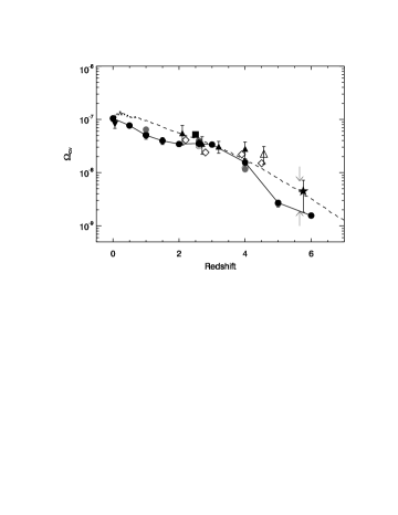
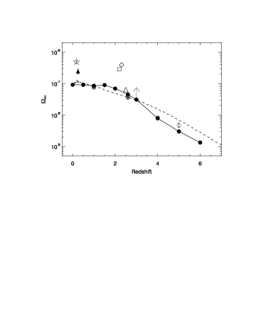
Figure 17: Top left: redshift evolution of $\Omega_{\rm CIV}$ from simulations: run “M” (filled black circles), run “MR” (open circles) and run “M2” (filled grey circles). Observational data are from Songaila (2005) (open diamonds), Becker et al. (2009) (arrows as limits), Pettini et al. (2003)(open triangle), Ryan-Weber et al. (2009) (filled star), Boksenberg et al. (2003) (filled upright triangles), Danforth & Shull (2008) (filled downright triangle) and Simcoe (2006)(filled square). The dashed curve is a simple physical model to explain the evolution of $\Omega_{\rm CIV}$ (see text in §3.2). Top right: redshift evolution of $\Omega_{\rm OVI}$. Observational data are from Carswell et al. (2002) (open square), Bergeron & Herbert-Fort (2005) (open diamond), Simcoe et al. (2002)(open triangle), Danforth & Shull (2008)(open star), Thom & Chen (2008b)(filled triangle) and Frank et al. (2008) (lower limit, arrow). Bottom left: different curves are the expected PDFs for $\Omega_{\rm CIV}$ at z=2.6, based on our simulations, for observational samples of various sizes (i.e., $\Delta X$ values). The solid vertical line indicates the median of the simulation results, whereas the vertical dashed line is Songaila (2005) value at z=2.5. Bottom right: the expected PDFs for $\Omega_{\rm OVI}$ at z=2.6. The solid vertical line indicates the median of the simulation results, whereas the vertical dashed line is Simcoe et al. (2002) value at z=2.5.

Figure 17 shows the evolution of the mass density contained in the C IV (left) and O VI (right) absorption lines, respectively. Considering the observational uncertainties and cosmic variance, it is very encouraging to see the excellent agreement between our simulated results and observations over the entire redshift range $z\sim 2-6$, where comparisons may be made.

As a new finding from our simulation, we note that a significant dispersion, i.e., cosmic variance, in $\Omega_{\rm CIV}$ is expected for available data samples with limited size (i.e., pathlength). In the bottom panels of Figure 17 we show the expected distribution based on our simulations for various sample sizes. We find that with $\Delta X=30$, the variance $\sigma=1.4\times 10^{-8}$ for C IV and $1.2\times 10^{-8}$ for O VI ; for $\Delta X=60$, $\sigma=1.0\times 10^{-8}$ for C IV and $8.5\times 10^{-9}$ for O VI ; with $\Delta X=160$, $\sigma=5.7\times 10^{-9}$ for C IV and $4.6\times 10^{-9}$ for O VI . Comparing C IV and O VI lines it is seen that the total amount of mass contained in the O VI line is comparable to that in the C IV line at all redshifts within a factor of 2 or so. Note that the size for the observational sample of Songaila (2005) is $\Delta X\leq 20$. Again, this suggests that some of the discrepancies between simulations and observations, and between observations may be accounted for by cosmic variance. For example, the slightly smaller value obtained from the observational sample of Songaila (2005) for $\Omega_{\rm CIV}$ is statistically consistent with simulations within $0.5\sigma$; the slightly larger value obtained from the observational sample of Simcoe et al. (2002) for $\Omega_{\rm OVI}$ is statistically consistent with simulations within $1\sigma$.

In agreement with observations, the mass density contained in the C IV absorption line is, within a factor of two, constant from $z=1$ to $z=4$ and subsequently drops by a factor of $\sim(10,20)$ by $z=(5,6)$. Some rather subtle difference between O VI and C IV lines may be noted. While the metal density contained in the C IV absorption line is nearly constant from $z=1$ to $z=4$, that plateau for the O VI line is attained only for $z=0-2$. Because the total amount of metals in the IGM has increased significantly in the redshift range $z=0-4$, it seems that the near constancy of $\Omega_{\rm CIV}$ at the redshift range $z=1-4$ and $\Omega_{\rm OVI}$ at the redshift range $z=0-2$ does not reflect the amount of metals in the IGM, which has already been pointed out earlier by Oppenheimer & Davé (2006). This probably reflects a “selection effect” of C IV systems of the overall metals in the IGM, which may be due to a combination of several different processes, including the evolution of the mean gas density as $(1+z)^{3}$, the evolution of the overdensity of the regions that produce C IV lines, the density dependence of the IGM metallicity and its evolution, the evolution of the radiation background and hierarchical build-up hence gravitational shock heating of the large-scale structure.

Our results contradict previous claims that observational data point towards a near constancy of $\Omega_{\rm CIV}$ with redshift (e.g., Songaila, 2001, 2005; Oppenheimer & Davé, 2006). However, more recent results have provided evidence of a downturn in $\Omega_{\rm CIV}$ towards $z\sim 6$. Becker et al. (2009) find no C IV absorbers in 4 sightlines towards $z\sim 6$ QSOs. They set limits on $\Omega_{\rm CIV}$ and attribute the downturn to a decline at least by a factor $\sim 4.4$ (to 95% confidence) in the number of C IV absorbers at $z=5.3-6$ as compared to $z=2-4.5$. The decline shown in Figure 16 is higher, at least a factor of $\sim 7$ for low column densities absorbers. Ryan-Weber et al. (2009) perform the most extensive survey of intergalactic metals at $z>5$, looking at the sightlines of 9 QSOs. They find evidence of a drop by a factor $\sim 3.5$ in the mass density of C IV from redshift $z=4.7$ to $z=5.7$. In comparison, we find a drop by a factor $\sim 1.7$ in $\Omega_{\rm CIV}$ in the interval $z=5-6$.

Figure 18: Left panel: the fraction of metals contained in C IV (circles) and O VI (squares) lines separately in terms of the overall amount of metals in the IGM at each redshift. Right panel: the fraction of metals contained in regions probed by C IV (circles) and O VI (squares) lines, respectively, in terms of the overall amount of metals in the IGM at each redshift.

Figure 19: shows the C IV ratio of $n_{C~{}IV\ }/n_{\rm C,tot}$ (open circles) and the O VI ratio of $n_{O~{}VI\ }/n_{\rm O,tot}$ (open squares) as a function of redshift. Note that at the optimal temperature with collisional ionization, $f_{max}$ for C IV and O VI is $29\%$ at $\log T_{\rm max}=5.00$ and $22\%$ at $\log T_{\rm max}=5.45$, respectively (Sutherland & Dopita, 1993).

The second point, perhaps the most overlooked, is that the amount of metals contained in the C IV and O VI absorption line is a very small fraction of the overall metals. The left panel of Figure 18 shows the ratios of mass density measured in the C IV (diamonds) and O VI lines (triangles) over the total amount of metals in the IGM as a function of redshift. We see that the amount of mass contained in the C IV line remains at $\sim 0.13\%$ within a dispersion of $40\%$, and at $\sim 0.13\%$ within a dispersion of $25\%$ for the O VI line. In the right panel of Figure 18 we show the amount of metals probed by each line as a function of redshift. Here is how we compute the metals probed by each line and use C IV as an example. For each detected C IV line, a range of spatial locations (i.e., gas cells along the line of sight) contributes to its column density (see Figures 4,5,6). Roughly speaking, the amount of metals effectively probed by the C IV line will be larger than the metals directly seen in the C IV line by a factor of $f=n_{C,tot}/n_{CIV}$ (a similar relation for the O VI line). This ratio $f$ for the C IV and O VI line is shown in Figure 19. One point worth noting is that for C IV there is an upturn of $f$ from $\sim 0.1$ at $z<2$ towards high redshift, reaching again the same value at $z=6$. This is caused from a transition from more collisionally dominated C IV absorber population at $z>4$ to a more photoionization dominated one at intermediate redshifts. The trend for the O VI line is much less pronounced, indicative of a dominance of collisionally ionized O VI absorbers over the entire redshift range $z=0-6$, with a trend that it is more so at higher redshift.

From the right panel of Figure 18 we see that, within a factor of $2$, the amount of metals probed by either C IV or O VI line is roughtly $2\%$. Combining the fact that the majority of C IV -producing regions have not collapsed and virialized (see Figure 9) and a small fraction of all metals is probed by C IV and O VI lines at all redshifts, C IV and O VI absorbers are “transients”; in other words, only a small fraction of metals in the IGM get “lit up” as the C IV or O VI line at any given time. As we demonstrated earlier, these regions that produce C IV absorption lines have a set of properties that seem to be created by a combination of physical processes including feedback shock heating and radiative cooling (see Figures 4,5,6). These close observations suggest that only a fraction of metals at any given time that has recently passed through shocks and cooled to an appropriate temperature shows up as C IV absorption lines. In this sense, C IV absorption lines trace the current feedback processes from star formation and how the current feedback energy and metal-enriched gas interact with the surrounding IGM. Similar statements about the transient nature could be made for the O VI line, except that the O VI line corresponds to somewhat different physical states of the shocked regions: they are slightly hotter in temperature and dynamically hotter.

Third, returning to Figure 17, we would like to emphasize that, consistent with recent observations (e.g., Becker et al., 2009; Ryan-Weber et al., 2009), there is indeed a sharp drop in $\Omega_{\rm CIV}$ from $z=3$ to $z=(4,5,6)$ by a factor of $\sim(2,10,20)$, respectively. This has less to do with the evolution of the total amount of metals produced, rather it is tracing the phase of C IV gas at any given time. At redshift $z\geq 3$, C IV lines at different redshifts appear to come from regions of comparable overdensity (see Figure 9) and comparable metallicity (see Figure 10). This allows us to test a very simple physical picture for the origin of C IV lines. They are produced by regions that were shock heated earlier by feedback shocks and have cooled to the temperature of $T\sim 10^{4.5}-10^{5}$K when they are seen, and the duration of each C IV line in this “C IV phase” would then be inversely proportional to the cooling time of the gas in this phase, which is proportional to $\Lambda^{-1}(T,Z)(1+z)^{-3}(1+\delta)^{-1}$, where $\Lambda(T,Z)$ is cooling function at temperature $T$ and metallicity $Z$ and the z-dependent term is due to density evolution with redshift. Then, the total amount of metals in C IV lines, $\Omega_{\rm CIV}$, will be proportional to $\dot{M}_{star}(z)\Lambda(T,Z)^{-1}(1+z)^{-3}(1+\delta)^{-1}$, where $\dot{M}_{star}(z)$ is the star formation rate at $z$. Taking $\delta$, $Z$ and $T$ as roughly being constant (see Figures  9, 10, 11), we have $\Omega_{\rm CIV}\propto\dot{M}_{star}(z)(1+z)^{-3}$, which is shown as the dashed curve on the left panel of Figure 17. It provides a reasonably good fit for the actual computed evolution of $\Omega_{\rm CIV}$.

3.3 Global Metal Enrichment of the IGM and Missing Metals

We now turn to present a global metal enrichment history of the IGM to supplement what is captured by the C IV and O VI absorption lines. As in Cen & Ostriker (1999b), in our analysis we divide the IGM into three components by temperature: (1) $T<10^{5}~{}$K cold-warm gas, which is in low density regions or cooling, star forming gas, (2) WHIM at $10^{7}~{}$K$>T>10^{5}~{}$K, (3) Hot X-ray emitting gas at $T>10^{7}$K. One additional component (4) is the baryons that have left the IGM and been condensed into stellar objects, which we designate as “stars”.

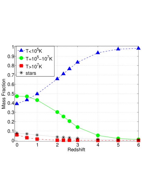
Figure 20: shows the evolution of baryons for the four mutually exclusive components: (1) $T<10^{5}~{}$K cold-warm gas, (2) WHIM at $10^{7}~{}$K$>T>10^{5}~{}$K, (3) Hot X-ray emitting gas at $T>10^{7}$K and (4) “stars”.

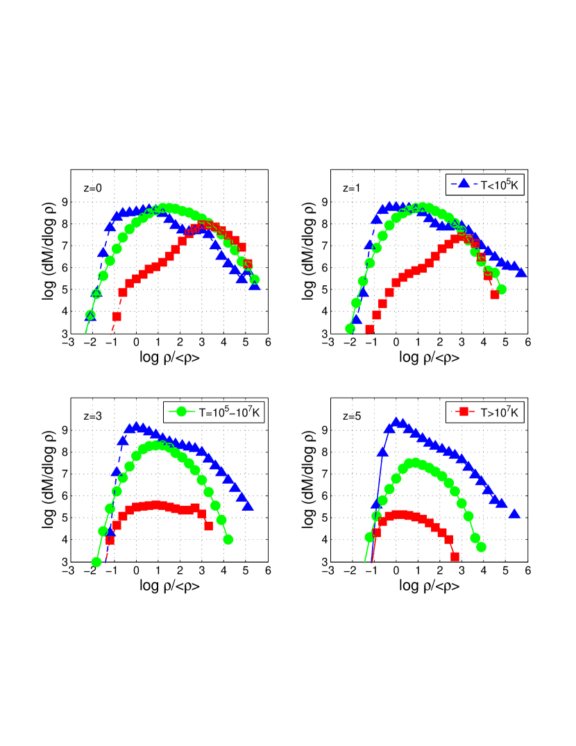
Figure 21: shows the mass distribution of the three IGM components - (1) cold-warm gas at $T<10^{5}~{}$K, (2) WHIM at $10^{7}~{}$K$>T>10^{5}~{}$K, (3) Hot X-ray emitting gas at $T>10^{7}$K - as a function of overdensity at four different redshifts $z=0,1,3,5$. Note that the area under each curve is proportional to the mass contained.

Figure 20 shows the evolution of these four components. The overall evolution of the four components are in good agreement with earlier findings (Cen & Ostriker, 1999b; Davé et al., 2001; Cen & Ostriker, 2006) and relevant observations (e.g., Fukugita et al., 1998). In particular, we see that $40-50\%$ of all baryons are in WHIM by the time $z=0$, which is in excellent agreement with our previous findings (Cen & Ostriker, 1999b; Davé et al., 2001; Cen & Ostriker, 2006). It is also noted that $\sim 40\%$ of the baryons at $z=0$ reside in a relatively cool but diffuse component with $T<10^{5}$K (the triangles in Figure 20). It is likely that a significant portion of this cool component at $z=0$, in the form of ${\rm Ly}\alpha$ forest, is already seen by UV observations (e.g., Penton et al., 2004). As we noted earlier, the strength of feedback from star formation is chosen to match the observed overall star formation history.

Each of the IGM components is composed of different regions that have gone through distinct evolutionary paths and thus spans a wide range in density, shown in Figure 21. The distribution of the cold-warm component (triangles) is always peaked at the mean density at all redshifts, reflecting the initial gaussian distribution of gas around the cosmic mean and indicating that the bulk of the IGM at mean density or lower has never been shock heated by either strong gravitational shocks or feedback shocks. The cold-warm gas extends to very high densities ($\geq 10^{5}$). It is interesting to note that the amount of cold-warm gas that could potentially feed the star formation, i.e., the cold-warm gas at density $\log\rho/\langle\rho\rangle\geq 2-3$, remains constant, within a factor of $\sim 2$, over the range redshift shown $z=0-5$. This is consistent with observations of the nearly non-evolving amount of gas probed by DLAs (e.g., Péroux et al., 2003; Zwaan et al., 2005; Rao et al., 2006; Prochaska & Wolfe, 2009; Noterdaeme et al., 2009). The physical relation between this apparently non-evolving gas and the precipitous drop of star formation rate at $z<1$ is currently unclear.

The distribution of the WHIM also appears to peak at a constant overdensity of about 10 times the mean density. This is rather intriguing. In order to properly interpret this interesting phenomenon it is useful to understand the heating sources of WHIM. There are two primary heating sources for WHIM: shocks due to the collapse of large-scale structure and GSW produced shocks. Earlier works have already shown that gravitational shock heating due to the formation of large-scale structure dominates the energy input for heating up and thus turning about $50\%$ of the IGM into WHIM by $z=0$ (Cen & Ostriker, 1999b; Davé et al., 2001; Cen & Ostriker, 2006). It is, however, expected that heating due to hydrodynamic shocks emanating from galactic superwinds become increasingly more important at higher redshifts. This is because the amount of energy from gravitational collapse of large-scale structure as well as the resulting shock velocity decreases steeply towards higher redshift. The reason for this is simple: in the standard cosmological model the amount of power is peaked at a wavelength of $\sim 300$Mpc/h and drops steeply towards small scales. To quantify the relative contribution of GSW in turning the IGM into WHIM, we compare the simulation with GSW feedback to that without GSW feedback (run N in Table 1). Then, we make the simple assertion that the difference in the amount of WHIM between the two simulations is due to GSW. Figure 22 shows the fraction of WHIM that is produced (cumulatively) by GSW as a function of redshift. Consistent with previous results (Cen & Ostriker, 1999b, 2006), the contribution from GSW to heating up WHIM by $z=0$ is subdominant at $10-20\%$. This relatively small contribution to WHIM from GSW can be understood based on simple energetics estimates. But we see the GSW fraction increases rapidly with increasing redshift. At redshift $z=1.5$ the GSW fraction is about $50\%$, then reaching $70\%$ at $z=3$ and $95\%$ at $z=5$. Thus, we see the primary heating source of WHIM at $z>1.5$ is GSW, whereas gravitational shocks due to structure formation are mostly responsible for heating the WHIM at $z<1.5$.

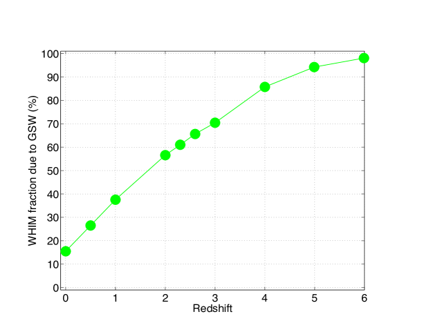
Figure 22: shows the (cumulative) fraction of WHIM that is produced by GSW as a function of redshift.

From Figure 21 it seems clear that WHIM does not distinguish between gravitational shocks and feedback shocks. In both cases shocks have largely stopped at overdensity of about $10$. Let us try to understand why that happened. First we note that the shocks originate approximately from the central regions of filaments, where pancakes collapse and shock for the case of gravitational shocks and galaxies are generally located for the case of GSW shocks. For gas shock heated to $10^{5}$K the shock velocity is roughly $70{\rm\,km/s}$. With that velocity the shock will be able to travel roughly $700(1+z)^{-1}$kpc comoving over the Hubble time at any redshift. Therefore, one should expect to see shocks have reached a few hundred kpc comoving at any redshift, which are about one to a few times the virial radius of typical large galaxies, which in turn correspond an overdensity in the vicinity of $10$ and are thus in good agreement with simulation results. Some shocks penetrate deeper into the IGM, especially along directions with lower densities and steeper density gradients, as seen in Figure 3; but the amount of mass effected in these low density regions is small, corresponding to the sharp drop of WHIM mass at the low density end (Figure 21). This last point is best corroborated by the distribution of the hot gas at high redshift ($z=3,5$), in the bottom two panels of Figure 21. There we see a small amount of hot gas heated up by GSW shocks is indeed produced in regions of density lower than the mean density and traces a larger amount of WHIM gas that is also produced there. At $z\leq 1$, some comparable, small amount of hot gas is still produced at low density regions. But the vast majority of hot X-ray emitting gas is now residing in the deep potential wells of X-ray clusters of galaxies, when the cluster scale turns nonlinear and collapses.

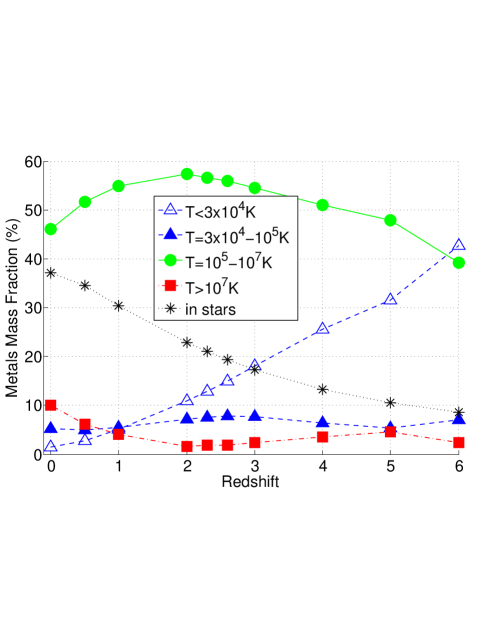
Figure 23: shows the evolution of fractions of all metals produced that are contained in each of the five components, as a function of redshift: (1C) $T<3\times 10^{4}~{}$K cold gas, (1W) $T=3\times 10^{4}-10^{5}~{}$K warm gas, (2) WHIM at $10^{7}~{}$K$>T>10^{5}~{}$K, (3) Hot X-ray emitting gas at $T>10^{7}$K, (4) “stars”.

Having obtained an overview of the thermal history of the IGM, we now turn to the metal story. We will first focus our attention on the WHIM here, because that is where most of the energy and metal exchanges between galaxies and the IGM take place, as shown in Figure 21. Observationally, integrating the observed star formation rate history from high redshift down to $z=2.5$ suggests that the vast majority (possibly $\geq 80\%$) of cosmic metals at $z\sim 2.5$ appear to be missing (e.g., Pagel, 1999; Pettini, 1999). Note that this conclusion is insensitive to the choice of IMF, since both UV light and metals are, to zeroth order, produced by the same massive stars. Metals that have been accounted for in the estimates include those in stars of Lyman break galaxies (LBG), damped Lyman alpha systems (DLAs) and ${\rm Ly}\alpha$ forest, i.e., cold-warm gas and stars. Given the dominant heating of WHIM by GSW, one may immediately ask: Could a significant fraction of metals that accompanies the GSW energy be heated up and in a phase like WHIM that is different from those where metals have been inventoried? To better address this open question, we further break down the IGM component (1) ($T<10^{5}~{}$K cold-warm gas) into two sub-components with (1C) ($T<3\times 10^{4}$K cold gas) and (1W) ($T=3\times 10^{4}-10^{5}$K warm gas). The purpose of this finer division is to separate out the cold gas (1C), which can be more appropriately identified with ${\rm Ly}\alpha$ forest clouds and DLAs. The results are shown in Figure 23. We see that about one third of all metals produced by $z=0$ is locked up in stars, decreasing monotonically towards high redshift, dropping to about $10\%$ by $z=5$. The fraction of metals in the hot X-ray emitting component is at about $10\%$ level at $z=0$, plummeting to about $2\%$ at $z=2$ and slowly rising back to about $6\%$ at $z=6$. It is likely that the metal fraction in the hot X-ray component at $z<1$ be somewhat underestimated given the relatively moderate simulation boxsize. The remaining metals are in the general photoionized ${\rm Ly}\alpha$ forest and the WHIM. At $z=6$ the ${\rm Ly}\alpha$ forest ($T<3\times 10^{4}$K, open triangles) contains about $43\%$ of all metals, while WHIM ($T=10^{5}-10^{7}$K, open circles), and warm IGM ($T=3\times 10^{4}-10^{5}$K, solid triangles) contain $39\%$ and $7\%$, respectively. But the fraction of metals in the ${\rm Ly}\alpha$ forest decreases steadily with time and becomes a minor component by $z=0$ at $<3\%$. Most of the metals is seen to be contained in the WHIM at all times below redshift five at $50-60\%$, peaking at $\sim 60\%$ at redshift $z\sim 2$. In total, the amount of metals contained in the IGM with temperature $T>3\times 10^{4}$ constitutes about 2/3 of all metals produced by $z=2.5$. Metals in this temperature range were not accounted for in the quoted observational inventory at $z=2.5$. Thus, it seems probable that the missing metals problem at $z=2-3$ can be largely rectified, if one counts the metals in the IGM at $T>3\times 10^{4}$K.

By now we have learned that a large amount of metals could be hidden in the WHIM of temperature $10^{5}-10^{7}$K spanning a wide range in density. Since the metallicity is a strong function of density, it is still unclear the location of the WHIM that dominates the missing metals. Figure 24 shows the mean metallicity of the three IGM components as a function of overdensity at four different redshifts. It is evident that within each IGM component there is a wide range in metallicity that is a non-trivial function of overdensity. Let us examine their behaviors in detail. For all three IGM components there is a strong correlation between the mean metallicity and overdensity at overdensity $\delta\geq 10$ and they converge at the highest density. While the metallicity of the cold-warm gas at the high density end remains at about solar at high density, its mean metallicity at the low overdensity drops rapidly with increasing redshift. For example, at $\delta=10$, the mean metallicity is (-2, -2.5, -3, -4) in solar units at $z=(0,1,3,5)$.

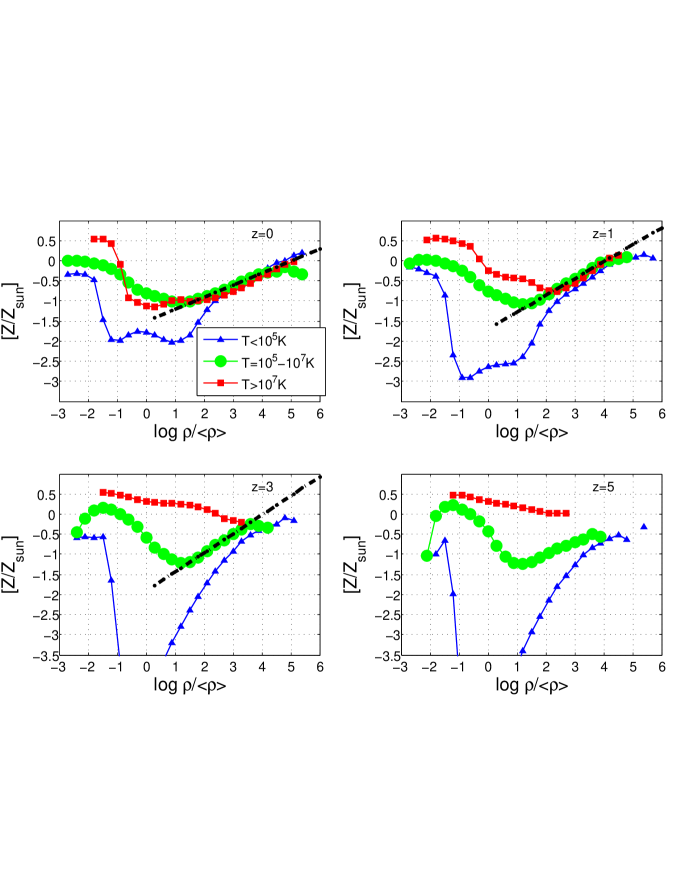
Figure 24: shows the metallicity of the three IGM components - (1) cold-warm gas at $T<10^{5}~{}$K, (2) WHIM at $10^{7}~{}$K$>T>10^{5}~{}$K, (3) Hot X-ray emitting gas at $T>10^{7}$K - as a function of overdensity at four different redshifts $z=0,1,3,5$.

One may notice that all three distributions exhibit a minimum metallicity at some intermediate density range, $\delta=0.1-10$ for the cold warm-gas, $\delta=10$ for the WHIM and $\delta=1-100$ for hot gas (only at $z=0-1$). This is entirely in agreement with the physical picture that we described earlier for the GSW shock propagation through the IGM. Figure 24 confirms that the transformation of cold gas to WHIM roughly stops at $\delta=10$. Additional metal-enriched gas is further transported along some directions, such as those perpendicular to the filaments, to very low density regions and enrich these regions to higher metallicity (due to a negligible amount of pre-existing gas there). The behavior of cold and hot components at the low density end can be understood in the same way as the WHIM. The metallicity of hot gas at the centers of clusters of galaxies (at overdensity $\rho/\langle\rho\rangle\geq 500$) appear to stay in narrow range around $[Z/{\rm\,Z_{\odot}}]\sim-0.5$ over the redshift range $z=0-1$, consistent with observations (e.g., Arnaud et al., 1994; Mushotzky et al., 1996; Tamura et al., 1996; Mushotzky & Loewenstein, 1997). There is some indication of a still higher metallicity towards higher density regions, which may be in agreement with observations (e.g., Iwasawa et al., 2001). The metallicity of the WHIM at the peak of its mass distribution ($\rho/\langle\rho\rangle\sim 10$) at $z=0$ is $[Z/{\rm\,Z_{\odot}}]\sim-1$, in good agreement with observations (e.g., Danforth & Shull, 2005). We find that the following formula fits well the metallicity of the WHIM as a function of overdensity $\rho/\langle\rho\rangle$ at the redshift range $z=0-3$:

$$[Z/Z_{\odot}]_{WHIM}=-1.2-0.08z+(0.3+0.12z^{1/3})(\log\rho/\langle\rho\rangle-1),$$ (6)

which are shown as the straight lines in the three panels of Figure 24.

Figure 25: shows the distributions of metals mass for the three IGM components - (1) cold-warm gas at $T<10^{5}~{}$K, (2) WHIM at $10^{7}~{}$K$>T>10^{5}~{}$K, (3) Hot X-ray emitting gas at $T>10^{7}$K - as a function of overdensity at four different redshifts $z=0,1,3,5$. Note that the area under each curve is proportional to the metals mass contained.

We now examine directly the distribution of metal mass as a function of density for each IGM component, shown in Figure 25. A very interesting result is that at high redshift ($z=3,5$) the metals mass in the WHIM tends to peak at a somewhat lower overdensity than that for the overall WHIM mass, thanks to the upturn of metallicity of the WHIM at low overdensity end. Specifically, at $z=3-5$ it appears that the metals mass peaks at $\delta\sim 2$, whereas the total WHIM mass peaks at $\delta\sim 10$. This trend is reversed at lower redshift; for example, at $z=0$ the metals in WHIM is now broadly peaked at $\delta\sim 100$, while the WHIM mass peaks at $\delta\sim 10$. This reversal is likely due to accretion of metal-enriched gas onto high density regions during recent formation of large-scale structures. Quantitatively, we find that, at $z=2.5$, only about $15\%$ of the metals in warm and WHIM gas is located within virialized regions. About $73\%$ of the metals in warm and WHIM gas resides in the IGM with $\delta=1-100$, with the remaining $12\%$ in underdense regions. This confirms an earlier expectation that some of the missing metals may be in the hot halos of galaxies (e.g., Pettini, 1999; Ferrara et al., 2005); but that accounts for only a small fraction of the total missing metals. Combining with our earlier statements on missing metals at $z=2-3$, our finding on missing metals is that most of the missing metals are in the warm and WHIM gas with moderate overdensity broadly distributed between $\delta\sim 1-10$.

Figure 26: shows metallicity evolution as a function of redshift at four fixed densities, $\rho /⟨\rho ⟩=$

References

- Adelberger et al. (2003) Adelberger, K. L., Steidel, C. C., Shapley, A. E., & Pettini, M. 2003, ApJ, 584, 45
- Aguirre et al. (2008) Aguirre, A., Dow-Hygelund, C., Schaye, J., & Theuns, T. 2008, ApJ, 689, 851
- Aguirre et al. (2001) Aguirre, A., Hernquist, L., Schaye, J., Katz, N., Weinberg, D. H., & Gardner, J. 2001, ApJ, 561, 521
- Aguirre et al. (2005) Aguirre, A., Schaye, J., Hernquist, L., Kay, S., Springel, V., & Theuns, T. 2005, ApJ, 620, L13
- Arnaud et al. (1994) Arnaud, K. A., Mushotzky, R. F., Ezawa, H., Fukazawa, Y., Ohashi, T., Bautz, M. W., Crewe, G. B., Gendreau, K. C., Yamashita, K., Kamata, Y., & Akimoto, F. 1994, ApJ, 436, L67
- Bahcall & Spitzer (1969) Bahcall, J. N. & Spitzer, Jr., L. 1969, ApJ, 156, L63+
- Barger et al. (2000) Barger, A. J., Cowie, L. L., & Richards, E. A. 2000, AJ, 119, 2092
- Becker et al. (2009) Becker, G. D., Rauch, M., & Sargent, W. L. W. 2009, ApJ, 698, 1010
- Bergeron et al. (2002) Bergeron, J., Aracil, B., Petitjean, P., & Pichon, C. 2002, A&A, 396, L11
- Bergeron & Herbert-Fort (2005) Bergeron, J. & Herbert-Fort, S. 2005, ArXiv Astrophysics e-prints
- Blanchard et al. (1992) Blanchard, A., Valls-Gabaud, D., & Mamon, G. A. 1992, A&A, 264, 365
- Boksenberg et al. (2003) Boksenberg, A., Sargent, W. L. W., & Rauch, M. 2003, ArXiv Astrophysics e-prints
- Bouwens et al. (2005) Bouwens, R. J., Illingworth, G. D., Thompson, R. I., & Franx, M. 2005, ApJL, 624, L5
- Burles et al. (2001) Burles, S., Nollett, K. M., & Turner, M. S. 2001, ApJ, 552, L1
- Carswell et al. (2002) Carswell, B., Schaye, J., & Kim, T. 2002, ApJ, 578, 43
- Cen et al. (1995) Cen, R., Kang, H., Ostriker, J. P., & Ryu, D. 1995, ApJ, 451, 436
- Cen et al. (1994) Cen, R., Miralda-Escude, J., Ostriker, J. P., & Rauch, M. 1994, ApJ, 437, L9
- Cen et al. (2005) Cen, R., Nagamine, K., & Ostriker, J. P. 2005, ApJ, 635, 86
- Cen & Ostriker (1999a) Cen, R. & Ostriker, J. P. 1999a, ApJ, 519, L109
- Cen & Ostriker (1999b) —. 1999b, ApJ, 514, 1
- Cen & Ostriker (2006) —. 2006, ApJ, 650, 560
- Cen et al. (2001) Cen, R., Tripp, T. M., Ostriker, J. P., & Jenkins, E. B. 2001, ApJ, 559, L5
- Chaffee et al. (1986) Chaffee, Jr., F. H., Foltz, C. B., Bechtold, J., & Weymann, R. J. 1986, ApJ, 301, 116
- Cole (1991) Cole, S. 1991, ApJ, 367, 45
- Cole et al. (2001) Cole, S., Norberg, P., Baugh, C. M., Frenk, C. S., Bland-Hawthorn, J., Bridges, T., Cannon, R., Colless, M., Collins, C., Couch, W., Cross, N., Dalton, G., De Propris, R., Driver, S. P., Efstathiou, G., Ellis, R. S., Glazebrook, K., Jackson, C., Lahav, O., Lewis, I., Lumsden, S., Maddox, S., Madgwick, D., Peacock, J. A., Peterson, B. A., Sutherland, W., & Taylor, K. 2001, MNRAS, 326, 255
- Cooksey et al. (2009) Cooksey, K. L., Thom, C., Prochaska, J. X., & Chen, H. 2009, ArXiv e-prints
- Cowie et al. (1999) Cowie, L. L., Songaila, A., & Barger, A. J. 1999, AJ, 118, 603
- Dalla Vecchia & Schaye (2008) Dalla Vecchia, C. & Schaye, J. 2008, MNRAS, 387, 1431
- Danforth & Shull (2005) Danforth, C. W. & Shull, J. M. 2005, ApJ, 624, 555
- Danforth & Shull (2008) —. 2008, ApJ, 679, 194
- Davé (2008) Davé, R. 2008, MNRAS, 385, 147
- Davé et al. (2001) Davé, R., Cen, R., Ostriker, J. P., Bryan, G. L., Hernquist, L., Katz, N., Weinberg, D. H., Norman, M. L., & O’Shea, B. 2001, ApJ, 552, 473
- D’Odorico et al. (2009) D’Odorico, V., Calura, F., Cristiani, S., & Viel, M. 2009, ArXiv e-prints
- Ferland et al. (1998) Ferland, G. J., Korista, K. T., Verner, D. A., Ferguson, J. W., Kingdon, J. B., & Verner, E. M. 1998, PASP, 110, 761
- Ferrara et al. (2005) Ferrara, A., Scannapieco, E., & Bergeron, J. 2005, ApJ, 634, L37
- Frank et al. (2008) Frank, S., Mathur, S., & York, D. G. 2008, ArXiv e-prints
- Fukugita et al. (1998) Fukugita, M., Hogan, C. J., & Peebles, P. J. E. 1998, ApJ, 503, 518
- Gabasch et al. (2004) Gabasch, A., Salvato, M., Saglia, R. P., Bender, R., et al. 2004, ApJ, 616, L83
- Giavalisco et al. (2004) Giavalisco, M., Dickinson, M., Ferguson, H. C., Ravindranath, S., Kretchmer, C., Moustakas, L. A., Madau, P., Fall, M., et al. 2004, ApJ, 600, L103
- Gnedin & Ostriker (1997) Gnedin, N. Y. & Ostriker, J. P. 1997, ApJ, 486, 581
- Haardt & Madau (1996) Haardt, F. & Madau, P. 1996, ApJ, 461, 20
- Heavens et al. (2004) Heavens, A. F., Panter, B., Jimenez, R., & Dunlop, J. 2004, Nature, 428, 625
- Heckman (2001) Heckman, T. M. 2001, in Astronomical Society of the Pacific Conference Series, Vol. 240, Gas and Galaxy Evolution, ed. J. E. Hibbard, M. Rupen, & J. H. van Gorkom, 345
- Hopkins et al. (2006) Hopkins, P. F., Hernquist, L., Cox, T. J., Robertson, B., Di Matteo, T., & Springel, V. 2006, ApJ, 639, 700
- Hui & Gnedin (1997) Hui, L. & Gnedin, N. Y. 1997, MNRAS, 292, 27
- Iwasawa et al. (2001) Iwasawa, K., Fabian, A. C., Allen, S. W., & Ettori, S. 2001, MNRAS, 328, L5
- Katz et al. (1996) Katz, N., Weinberg, D. H., & Hernquist, L. 1996, ApJS, 105, 19
- Komatsu et al. (2009) Komatsu, E., Dunkley, J., Nolta, M. R., Bennett, C. L., Gold, B., Hinshaw, G., Jarosik, N., Larson, D., Limon, M., Page, L., Spergel, D. N., Halpern, M., Hill, R. S., Kogut, A., Meyer, S. S., Tucker, G. S., Weiland, J. L., Wollack, E., & Wright, E. L. 2009, ApJS, 180, 330
- Krumholz & Tan (2007) Krumholz, M. R. & Tan, J. C. 2007, ApJ, 654, 304
- Li et al. (2008) Li, S., Li, H., & Cen, R. 2008, ApJS, 174, 1
- Lilly et al. (1996) Lilly, S. J., Fèvre, O. L., Hammer, F., & Crampton, D. 1996, ApJ, 460, L1
- Lu et al. (1998) Lu, L., Sargent, W. L. W., Barlow, T. A., & Rauch, M. 1998, ArXiv Astrophysics e-prints
- Mac Low & Ferrara (1999) Mac Low, M. & Ferrara, A. 1999, ApJ, 513, 142
- Mathur et al. (2003) Mathur, S., Weinberg, D. H., & Chen, X. 2003, ApJ, 582, 82
- McDonald et al. (2000) McDonald, P., Miralda-Escudé, J., Rauch, M., Sargent, W. L. W., Barlow, T. A., Cen, R., & Ostriker, J. P. 2000, ApJ, 543, 1
- Mushotzky et al. (1996) Mushotzky, R., Loewenstein, M., Arnaud, K. A., Tamura, T., Fukazawa, Y., Matsushita, K., Kikuchi, K., & Hatsukade, I. 1996, ApJ, 466, 686
- Mushotzky & Loewenstein (1997) Mushotzky, R. F. & Loewenstein, M. 1997, ApJ, 481, L63+
- Nakamura et al. (2004) Nakamura, O., Fukugita, M., Brinkmann, J., & Schneider, D. P. 2004, AJ, 127, 2511
- Nicastro et al. (2009) Nicastro, F., Krongold, Y., Fields, D., Conciatore, M. L., Zappacosta, L., Elvis, M., Mathur, S., & Papadakis, I. 2009, ArXiv e-prints
- Norman et al. (2004) Norman, C., Ptak, A., Hornschemeier, A., Hasinger, G., Bergeron, J., Comastri, A., Giacconi, R., Gilli, R., et al. 2004, ApJ, 607, 721
- Norris et al. (1983) Norris, J., Peterson, B. A., & Hartwick, F. D. A. 1983, ApJ, 273, 450
- Noterdaeme et al. (2009) Noterdaeme, P., Petitjean, P., Ledoux, C., & Srianand, R. 2009, A&A, 505, 1087
- Oppenheimer & Davé (2006) Oppenheimer, B. D. & Davé, R. 2006, MNRAS, 373, 1265
- Ouchi et al. (2004) Ouchi, M., Shimasaku, K., Okamura, S., Furusawa, H., Kashikawa, N., Ota, K., Doi, M., Hamabe, M., Kimura, M., Komiyama, Y., Miyazaki, M., Miyazaki, S., Nakata, F., Sekiguchi, M., Yagi, M., & Yasuda, N. 2004, ApJ, 611, 660
- Pagel (1999) Pagel, B. E. J. 1999, ArXiv Astrophysics e-prints
- Pen (1999) Pen, U. 1999, ApJ, 510, L1
- Penton et al. (2004) Penton, S. V., Stocke, J. T., & Shull, J. M. 2004, ApJS, 152, 29
- Péroux et al. (2003) Péroux, C., McMahon, R. G., Storrie-Lombardi, L. J., & Irwin, M. J. 2003, MNRAS, 346, 1103
- Pettini (1999) Pettini, M. 1999, in Chemical Evolution from Zero to High Redshift, ed. J. R. Walsh & M. R. Rosa, 233–+
- Pettini et al. (2003) Pettini, M., Madau, P., Bolte, M., Prochaska, J. X., Ellison, S. L., & Fan, X. 2003, ApJ, 594, 695
- Pettini et al. (1997) Pettini, M., Smith, L. J., King, D. L., & Hunstead, R. W. 1997, ApJ, 486, 665
- Prochaska et al. (2003) Prochaska, J. X., Gawiser, E., Wolfe, A. M., Castro, S., & G., G. D. 2003, ApJ, 595, L9
- Prochaska & Wolfe (2009) Prochaska, J. X. & Wolfe, A. M. 2009, ApJ, 696, 1543
- Rao et al. (2006) Rao, S. M., Turnshek, D. A., & Nestor, D. B. 2006, ApJ, 636, 610
- Rauch et al. (1996) Rauch, M., Sargent, W. L. W., Womble, D. S., & Barlow, T. A. 1996, ApJ, 467, L5+
- Reddy et al. (2005) Reddy, N. A., Erb, D. K., Steidel, C. C., Shapley, A. E., Adelberger, K. L., & Pettini, M. 2005, ApJ, 633, 748
- Ryan-Weber et al. (2006) Ryan-Weber, E. V., Pettini, M., & Madau, P. 2006, MNRAS, 371, L78
- Ryan-Weber et al. (2009) Ryan-Weber, E. V., Pettini, M., Madau, P., & Zych, B. J. 2009, MNRAS, 395, 1476
- Schaye et al. (2003) Schaye, J., Aguirre, A., Kim, T., Theuns, T., Rauch, M., & Sargent, W. L. W. 2003, ApJ, 596, 768
- Schramm & Turner (1998) Schramm, D. N. & Turner, M. S. 1998, Reviews of Modern Physics, 70, 303
- Shen et al. (2010) Shen, S., Wadsley, J., & Stinson, G. 2010, MNRAS, 407, 1581
- Simcoe (2006) Simcoe, R. A. 2006, ApJ, 653, 977
- Simcoe et al. (2002) Simcoe, R. A., Sargent, W. L. W., & Rauch, M. 2002, ApJ, 578, 737
- Simcoe et al. (2004) —. 2004, ApJ, 606, 92
- Songaila (2001) Songaila, A. 2001, ApJ, 561, L153
- Songaila (2005) —. 2005, AJ, 130, 1996
- Springel & Hernquist (2003) Springel, V. & Hernquist, L. 2003, MNRAS, 339, 289
- Steidel et al. (1999) Steidel, C. C., Adelberger, K. L., Giavalisco, M., Dickinson, M., & Pettini, M. 1999, ApJ, 519, 1
- Steidel & Sargent (1992) Steidel, C. C. & Sargent, W. L. W. 1992, ApJS, 80, 1
- Steinmetz (1996) Steinmetz, M. 1996, MNRAS, 278, 1005
- Sutherland & Dopita (1993) Sutherland, R. S. & Dopita, M. A. 1993, ApJS, 88, 253
- Tamura et al. (1996) Tamura, T., Day, C. S., Fukazawa, Y., Hatsukade, I., Ikebe, Y., Makishima, K., Mushotzky, R. F., Ohashi, T., Takenaka, K., & Yamashita, K. 1996, PASJ, 48, 671
- Theuns et al. (2002a) Theuns, T., Schaye, J., Zaroubi, S., Kim, T.-S., Tzanavaris, P., & Carswell, B. 2002a, ApJ, 567, L103
- Theuns et al. (2002b) Theuns, T., Viel, M., Kay, S., Schaye, J., Carswell, R. F., & Tzanavaris, P. 2002b, ApJ, 578, L5
- Thom & Chen (2008a) Thom, C. & Chen, H. 2008a, ApJS, 179, 37
- Thom & Chen (2008b) —. 2008b, ApJ, 683, 22
- Tripp et al. (2008) Tripp, T. M., Sembach, K. R., Bowen, D. V., Savage, B. D., Jenkins, E. B., Lehner, N., & Richter, P. 2008, ApJS, 177, 39
- Tytler & Fan (1994) Tytler, D. & Fan, X. 1994, ApJ, 424, L87
- White & Frenk (1991) White, S. D. M. & Frenk, C. S. 1991, ApJ, 379, 52
- Wu et al. (2001) Wu, K. K. S., Fabian, A. C., & Nulsen, P. E. J. 2001, MNRAS, 324, 95
- Yepes et al. (1997) Yepes, G., Kates, R., Khokhlov, A., & Klypin, A. 1997, MNRAS, 284, 235
- Young et al. (1982) Young, P., Sargent, W. L. W., & Boksenberg, A. 1982, ApJS, 48, 455
- Zhang et al. (2009) Zhang, W., Li, C., Kauffmann, G., Zou, H., Catinella, B., Shen, S., Guo, Q., & Chang, R. 2009, MNRAS, 397, 1243
- Zwaan et al. (2005) Zwaan, M. A., Meyer, M. J., Staveley-Smith, L., & Webster, R. L. 2005, MNRAS, 359, L30