Optimization of dividend and reinsurance strategies under ruin probability constraint

Abstract.

This paper considers nonlinear regular-singular stochastic optimal control of large insurance company. The company controls the reinsurance rate and dividend payout process to maximize the expected present value of the dividend pay-outs until the time of bankruptcy. However, if the optimal dividend barrier is too low to be acceptable, it will make the company result in bankruptcy soon. Moreover, although risk and return should be highly correlated, over-risking is not a good recipe for high return, the supervisors of the company have to impose their preferred risk level and additional charge on firm seeking services beyond or lower than the preferred risk level. These indeed are nonlinear regular-singular stochastic optimal problems under ruin probability constraints. This paper aims at solving this kind of the optimal problems, that is, deriving the optimal retention ratio,dividend payout level, optimal return function and optimal control strategy of the insurance company. As a by-product, the paper also sets a risk-based capital standard to ensure the capital requirement of can cover the total given risk, and the effect of the risk level on optimal retention ratio, dividend payout level and optimal control strategy are also presented. MSC(2000): Primary 91B30,91B70,93E20; Secondary 60H30, 60H10. Keywords: Nonlinear regular-singular stochastic optimal control; Ruin probability ; Optimal retention ratio; Optimal dividend payout; Optimal return function.

1. Introduction

In the present paper we consider nonlinear stochastic optimal control of insurance company. The company controls the reinsurance rate and dividend payout process to maximize the expected present value of the dividend pay-outs until the time of bankruptcy. It is well known that over-risking is not a good recipe for high return although risk and return should be highly correlated. In fact, to reduce the risk, a risk-averse re-insurers may have their preferred risk level and impose additional service charge on firms seeking services beyond the target level, other re-insurers may demand additional charges for those seeking services with risk level lower than its preferred level as an aggressive move to gain market shares. This indeed is nonlinear regular-singular stochastic optimal problem. The objective of the company is to find a strategy, consisting of optimal retention ratio and dividend payment scheme, which maximizes the expected total discounted dividend pay-outs until the time of bankruptcy. This is a mixed regular-singular control problem on diffusion model which has been a renewed interest recently,We refer readers to He, Liang and et al. [12, 13, 14](2008,2009)and references therein, Højgaard and Taksar[16, 17, 15](1999, 1998, 2001),Asmussen et all[2, 3](1997,2000), Taksar[28](2000), Guo Xin, Liu Jun and Zhou Xunyu[11](2004), Harrison and Taksar[19](1983), Paulsen and Gjessing [24](1997), and Radner and Sheep[25](1996),and other authors’ works. Recent surveys can be found in Avanzi [4].

However, we notice that the optimal dividend barrier in the nonlinear regular-singular stochastic optimal problem may be so low that it would make the company result in bankruptcy soon( see theorem 4.1), the company may reject this optimal control strategy and may be prohibited to pay dividend at such a low barrier because the insurance company is a business affected with a public interest, and insureds and policy-holders should be protected against insurer insolvencies (see Williams and Heins[30](1985), Riegel and Miller[26](1963), and Welson and Taylor[29](1959)). The strategy, making the company go bankrupt before termination of contract between insurer and policy holders or the strategy of low solvency(1 minus ruin probability(see [5])), is not the best way and should be prohibited even though it can win the highest profit. So the supervisor of the company will impose some constraints on its ruin probability and find the best equilibrium strategy between making profit and improving security. These are turned out to be nonlinear regular-singular stochastic optimal problems under low ruin probability constraint. This paper aims at solving these kinds of stochastic optimal problems

Unfortunately, there are very few results concerning on these kinds of optimal control problem with lower ruin probability and higher security. He, Hou and Liang[13](2008) investigated the optimal control problem for linear Brownian model, Paulsen[22](2003) and Taksar and Markussen [6](2004) studied also similar optimal controls linear diffusion model via properties of return function. Since the model treated in the present paper is very complicate and different from He, Hou and Liang[13](2008) and Paulsen[22](2003), our results can not be directly deduced from the [13, 22]. Therefore, to solve these the problems we need to use initiated idea from the [13](2008), stochastic analysis and PDE method to establish a complete setting for further discussing optimal control problem of a large insurance company under lower ruin probability constraint. This paper is the first complete presentation of the topic, and the approach here is rather general, so we anticipate that it can deal with other models. We aim at deriving the optimal return function, the optimal retention rate and dividend payout level. The main result of this paper will be presented in section 3 below. As a by-product, the paper theoretically sets a risk-based capital standard to ensure the capital requirement of can cover the total given risk. Moreover, based on our main result, we also discuss how the risk affect the optimal reactions of the insurance company by the implicit types of solutions and how the optimal retention ratio, dividend payout level and risk-based capital standard are affected by risk faced by the insurance company, and how the initial capital and the premium rate impact on the company’s profit.

The paper is organized as follows: In next section, we establish nonlinear stochastic control model of a large insurance company with ruin probability constraint. In section 3 we present main result of this paper and its economic and financial interpretations, and discuss how the risk affect the optimal reactions of the insurance company by the implicit types of solutions and how the optimal retention ratio, dividend payout level and risk-based capital standard are affected by risk faced by the insurance company, and how the initial capital and the premium rate impact on the company’s profit. In section 4 we give analysis on risk of stochastic control model treated in the present paper to explain why we study nonlinear regular-singular stochastic optimal control of insurance company. In section 5 we give some numerical samples to portray how the risk impacts on optimal dividend payout level and risk-based capital based on PDE (6.25) below, and how the premium rate, preferred reinsurance level and volatility effect on the company’s profit. The proofs of theorems and lemmas which study properties of probability of bankruptcy and optimal return function will be given in section 6 and appendix.

2. Nonlinear Mathematical Model

To give a mathematical formulation of the stochastic control problem treated in this paper, let $(\Omega,\mathcal{F},\{\mathcal{F}_{t}\}_{t\geq 0},\mathbb{P})$ denote a filtered probability space. $\{\mathcal{W}_{t},t\geq 0\}$ is a standard Brownian motion on this probability space. $\mathcal{F}_{t}$ represents the information available at time $t$ and any decision is made based on this information. For the intuition of our diffusion model we start from the classical Cramér-Lundberg model of a reserve(risk) process to portray that if the insurance company shares risk with the reinsurance and takes no dividend pay-out then its reserve process can be approximated by the following diffusion process

$$dR_{t}=\mu_{1}U(t)dt+\sigma U(t)d\mathcal{W}_{t},$$ (2.1)

where $U(t)$ denotes retention level. In the classical Cramér-Lundberg model claims arrive according to a Poisson process $N_{t}$ with intensity $\lambda$ on $(\Omega,\mathcal{F},\{\mathcal{F}_{t}\}_{t\geq 0},\mathbb{P})$. The size of each claim is $X_{i}$. Positive random variables $X_{i}$ are i.i.d. and are independent of the Poisson process $N_{t}$ with finite first and second moments given by $\mu$ and $\sigma^{2}$ respectively. If there is no reinsurance, dividend pay-outs, the reserve (risk) process of insurance company is described by

$$r_{t}=r_{0}+pt-\sum^{N_{t}}_{i=1}X_{i},$$

where $p$ is the premium rate. If $\eta>0$ denotes the safety loading, the $p$ can be calculated via the expected value principle as

$$p=(1+\eta)\lambda\mu.$$

In a case where the insurance company shares risk with the reinsurance, the sizes of the claims held by the insurer become $X^{(U)}_{i}$, where $U$ is a (fixed) retention level. For proportional reinsurance, $U$ denotes the fraction of the claim covered by the insurance company . Consider the case of cheap reinsurance for which the reinsuring company uses the same safety loading as the insurance company, the reserve process of the insurance company is given by

$$r^{(U,\eta)}_{t}=u+p^{(U,\eta)}t-\sum^{N_{t}}_{i=1}X^{(U)}_{i},$$

where

$$p^{(U,\eta)}=(1+\eta)\lambda\mathbb{E}\{X^{(U)}_{i}\}.$$

Then by center limit theorem it is well known that for large enough $\lambda$

$$r_{t}^{(U,\eta)}\stackrel{{\scriptstyle d}}{{\approx}}BM(\mu Ut,\sigma^{2}U^{2}t).$$

in $\mathcal{D}[0,\infty)$ (the space of right continuous functions with left limits endowed with the skorohod topology), where $\mu=\eta\lambda E(X_{i})$, $\sigma=\sqrt{\lambda E(X_{i}^{2})}$ and $BM(\mu,\sigma^{2})$ stands for Brownian motion with the drift coefficient $\mu$ and diffusion coefficient $\sigma$ on $(\Omega,\mathcal{F},\{\mathcal{F}_{t}\}_{t\geq 0},\mathbb{P})$. So the passage to the limit works well in the presence of a big portfolios, the reserve (risk) process of the insurance company can be described by (2.1). We refer the reader for this fact and for the specifies of the diffusion approximations to Emanuel, Harrison and Taylor [7](1975), Grandell[8, 9, 10](1977,1978,1990), Harri-son [18](1985), Iglehart[20](1969), Schmidli[27](1994). It is well known that over-risking is not a good recipe for high return although risk and return are highly correlated. This leads to question how an optimal strategy would change when the risk and return are not linearly dependent on each other. Moreover, while a risk-averse re-insurers may have their preferred risk level and impose additional service charge on firms seeking services beyond the target level, other re-insurers may demand additional charges for those seeking services with risk level lower than its preferred level as an aggressive move to gain market shares. These make the reserve process of the company should be the following

$$dR(t)=[\mu_{1}U(t)-a(U(t)-p)^{2}]dt+\sigma U(t)d\mathcal{W}_{t},\ R(0)=x,$$ (2.2)

where p is the preferred reinsurance level imposed by the re-insurer and $a$ is the additional rate of charge for the deviation from the preferred level which ensures that larger deviation is penalized heavily. If we let $\mu=u_{1}+2ap$, $\delta=ap^{2}$, then the (2.2) becomes

$$dR_{t}=(\mu U(t)-aU^{2}(t)-\delta)dt+\sigma U(t)d\mathcal{W}_{t},\ \ R(0)=x,$$ (2.3)

A strategy $\pi$ is a pair of non-negative càdlàg $\mathcal{F}_{t}$-adapted processes $\{U_{\pi}(t),L_{t}^{\pi}\}$, where $U_{\pi}(t)\in[l,1](l>0)$ corresponds to the risk exposure at time $t$ and $L_{t}^{\pi}$ corresponds to the cumulative amount of dividend pay-outs distributed up to time $t$. A strategy $\pi=\{U_{\pi}(t),L_{t}^{\pi}\}$ is called admissible if $l\leq U_{\pi}(t)\leq 1$ and $L_{t}^{\pi}$ is a nonnegative, non-decreasing, right-continuous function. When $\pi$ is applied, the resulting reserve process is denoted by $\{R_{t}^{\pi}\}$. We assume that the initial reserve $R^{\pi}_{0}$ is a deterministic value $x$. In view of (2.3) the dynamics for $R_{t}^{\pi}$ is given by

$$dR^{\pi}_{t}=[\mu U_{\pi}(t)-a(U_{\pi}(t))^{2}-\delta]dt+\sigma U_{\pi}(t)d\mathcal{W}_{t}-dL^{\pi}_{t},\ R^{\pi}_{0}=x.$$ (2.4)

In this case, we assume the company needs to keep its reserve above $0$. The company is considered ruin as soon as the reserves fall below $0$. We define the time of bankruptcy by $\tau^{\pi}_{x}=\inf\{t\geq 0:R^{\pi}_{t}\leq 0\}$. Obviously, $\tau^{\pi}_{x}$ is an $\mathcal{F}_{t}$ -stopping time. So the management of the insurance company should maximize the expected present value of the dividend payout by control strategy $\pi$. Guo, Liu and Zhou[11] proved that there exists a dividend level $b_{0}$, control strategy $\pi^{*}_{b_{0}}$ and the time of bankruptcy $\tau_{x}^{b_{0}}$ maximizing the expected present value of the dividend payout before bankruptcy,

$$J(x,\pi) = {\bf E}\large[(\int_{0}^{\tau}e^{-cs}dL^{\pi}_{s})],$$ (2.5)

$$V(x,b_{0}) = \sup\limits_{\pi\in\Pi}J(x,\pi)=J(x,\pi^{*}_{b_{0}}),$$ (2.6)

where $c$ denotes the discount rate, $\Pi$ is the set of all admissible strategies. If the optimal dividend level $b_{0}$ is unacceptably low, then it will result in the company go to bankruptcy early ( see theorem 4.1 below). To take security and solvency into consideration and set a risk-based capital and dividend standard to ensure the capital and dividend requirement of can cover the total risk, we introduce our optimal control problem of nonlinear stochastic model (2.4) as follows.Let $\Pi_{b}=\{\pi\in\Pi:\int_{0}^{\infty}I_{\{s:R^{\pi}(s)<b\}}dL_{s}^{\pi}=0\}$ for $b\geq 0$ . Then it is easy to see that $\Pi=\Pi_{0}$ and $b_{1}>b_{2}\Rightarrow\Pi_{b_{1}}\subset\Pi_{b_{2}}$. For a given admissible strategy $\pi$ we define the optimal return function $V(x)$ by

$$J(x,\pi) = {\bf E}\big{\{}\int_{0}^{\tau^{\pi}_{x}}e^{-ct}dL_{t}^{\pi}\big{\}},$$

$$V(x,b) = \sup_{\pi\in\Pi_{b}}\{J(x,\pi)\},$$ (2.7)

$$V(x) = \sup_{b\in\mathfrak{B}}\{V(x,b)\}$$ (2.8)

and the optimal strategy $\pi^{*}$ by

$$J(x,\pi^{*})=V(x),$$ (2.9)

where

$$\mathfrak{B}:=\big{\{}b\ :\ \mathbb{P}[\tau_{b}^{\pi_{b}}\leq T]\leq\varepsilon\ ,\ J(x,\pi_{b})=V(x,b)\mbox{ and}\ \pi_{b}\in\Pi_{b}\big{\}},$$

$c>0$ is a discount rate, $\tau_{b}^{\pi_{b}}$ is the time of bankruptcy $\tau_{x}^{\pi_{b}}$ when the initial reserve $x=b$ and the control strategy is $\pi_{b}$. $1-\varepsilon$ is the standard of security and less than solvency for given risk level $\varepsilon>0$.

The main purpose of this paper is to derive the optimal return function $V(x)$, the optimal retention rate $U^{*}(t)$ and dividend payout level $b^{*}$ as well as a risk-based capital $x(\varepsilon,b^{*})$ to ensure the capital requirement of can cover the total risk $\varepsilon$.

3. Main result

In this section we first present main result of this paper, then give its economic and financial interpretations .

Theorem 3.1.

Let level of risk $\varepsilon\in(0,1)$ and time horizon $T$ be given. (i) If $\mathbf{P}[\tau_{b_{0}}^{\pi^{*}_{b_{0}}}\leq T]\leq\varepsilon$,then the optimal return function $V(x)$ is $f(b_{0},x)$ defined by (6.1) below, and $V(x)=f(b_{0},x)=J(x,\pi_{b_{o}}^{\ast})$. The optimal strategy $\pi_{b_{o}}^{\ast}$ is $\{U^{\ast}(R^{\pi_{b_{o}}^{\ast}}_{t}),L^{\pi_{b_{o}}^{\ast}}_{t}\}$, where $\{R^{\pi_{b_{o}}^{\ast}}_{t},L^{\pi_{b_{o}}^{\ast}}_{t}\}$ is uniquely determined by the following stochastic differential equation

$$\left\{\begin{array}[]{l l l}dR_{t}^{\pi_{b_{o}}^{\ast}}=(\mu U^{*}_{b_{0}}(R^{\pi_{b_{o}}^{\ast}}_{t})-a{U^{*}_{b_{0}}}^{2}(R^{\pi_{b_{o}}^{\ast}}_{t})-\delta)dt+\sigma U^{*}_{b_{0}}(R^{\pi_{b_{o}}^{\ast}}_{t})d{W}_{t}-dL_{t}^{\pi_{b_{o}}^{\ast}},\\ R_{0}^{\pi_{b_{o}}^{\ast}}=x,\\ 0\leq R^{\pi_{b_{o}}^{\ast}}_{t}\leq b_{0},\\ \int^{\infty}_{0}I_{\{t:R^{\pi_{b_{o}}^{\ast}}_{t}<b_{0}\}}(t)dL_{t}^{\pi_{b_{o}}^{\ast}}=0.\end{array}\right.$$ (3.5)

The solvency of the company is bigger than $1-\varepsilon$. (ii)If $\mathbf{P}[\tau_{b_{0}}^{\pi^{*}_{b_{0}}}\leq T]>\varepsilon$, there is a unique optimal dividend $b^{\ast}(\geq b_{0})$ satisfying $\mathbb{P}[\tau_{b^{\ast}}^{\pi_{b^{*}}^{\ast}}\leq T]=\varepsilon$. The optimal return function $V(x)$ is $g(x,b^{*})$ defined by (6.8), that is,

$$V(x)=g(x,b^{*})=\sup_{b\in\mathfrak{B}}\{V(x,b)\},$$ (3.6)

and

$$b^{*}\in\mathfrak{B}:=\big{\{}b:\mathbb{P}[\tau_{b}^{\pi^{*}_{b}}\leq T]\leq\varepsilon,\ J(x,\pi^{*}_{b})=V(x,b)\mbox{ and}\ \pi^{*}_{b}\in\Pi_{b}\ \big{\}}.$$ (3.7)

The optimal strategy $\pi_{b^{*}}^{\ast}$ is $\{U^{\ast}_{b^{*}}(R^{\pi_{b^{*}}^{\ast}}_{t}),L^{\pi_{b^{*}}^{\ast}}_{t}\}$, where $\{R^{\pi_{b^{*}}^{\ast}}_{t},L^{\pi_{b^{*}}^{\ast}}_{t}\}$ is uniquely determined by the following stochastic differential equation

$$\left\{\begin{array}[]{l l l}dR_{t}^{\pi_{b^{*}}^{\ast}}=(\mu U^{*}_{b^{*}}(R^{\pi_{b^{*}}^{\ast}}_{t})-a{U^{*}_{b^{*}}}^{2}(R^{\pi_{b^{*}}^{\ast}}_{t})-\delta)dt+\sigma U^{*}_{b^{*}}(R^{\pi_{b^{*}}^{\ast}}_{t})d{W}_{t}-dL_{t}^{\pi_{b^{*}}^{\ast}},\\ R_{0}^{\pi_{b^{*}}^{\ast}}=x,\\ 0\leq R^{\pi_{b^{*}}^{\ast}}_{t}\leq b^{*},\\ \int^{\infty}_{0}I_{\{t:R^{\pi_{b^{*}}^{\ast}}_{t}<b^{*}\}}(t)dL_{t}^{\pi_{b^{*}}^{\ast}}=0.\end{array}\right.$$ (3.12)

The solvency of the company is $1-\varepsilon$. (3) Moreover,

$$\frac{g(x,b^{*})}{g(x,b_{0})}\leq 1.$$ (3.13)

Where $U^{*}_{b}(x)$ is defined by (6.21) and (6.29) below.

Economic and financial explanation of theorem 3.1 is as follows.(1) For a given level of risk and time horizon, if ruin probability is less than the level of risk, the optimal control problem of (2) and (2.8) is the traditional (2.5) and (2.6), the company has higher solvency, so it will have good reputation. The solvency constraints here do not work. This is a trivial case. (2) If ruin probability is large than the level of risk $\varepsilon$, the traditional optimal strategy will not meet the standard of security and solvency, the company needs to find a sub-optimal strategy $\pi_{b^{*}}^{\ast}$ to improve its solvency. The sub-optimal reserve process $R^{\pi_{b^{*}}^{\ast}}_{t}$ is a diffusion process reflected at $b^{*}$, the process $L^{\pi_{b^{*}}^{\ast}}_{t}$ is the process which ensures the reflection. The sub-optimal action is to pay out everything in excess of $b^{*}$ as dividend and pay no dividend when the reserve is below $b^{*}$, and $U_{b^{*}}^{*}(x)$ is the sub-optimal feedback control function. The solvency is $1-\varepsilon$. (3) On the one hand, the inequality (3.13) states that $\pi_{b^{*}}^{\ast}$ will reduce the company’s profit, on the other hand, in view of (3.13) and $\mathbb{P}[\tau_{b^{\ast}}^{\pi_{b^{*}}^{\ast}}\leq T]=\varepsilon$ as well as lemma 6.4 below, the cost of improving solvency is minimal $g(x,b_{0})-g(x,b^{*})$. Therefore the strategy $\pi_{b^{*}}^{\ast}$ is the best equilibrium action between making profit and improving solvency. (4) The risk-based capital $x(\varepsilon,b^{*})$ to ensure the capital requirement of can cover the total risk $\varepsilon$ can be determined by numerical solution of $1-\phi^{b^{*}}(x,b^{*})=\varepsilon$ based on (6.25). We see from the figure 5 that risk-based capital $x(\varepsilon,b^{*})$ decreases with risk $\varepsilon$, i.e., $x(\varepsilon,b^{*})$ increases with solvency , so does risk-based dividend level $b^{*}(\varepsilon)$ (see the figure 1). (5) We also see from the figures 2 and 4 below that the premium rate will increase the company’s profit, higher risk will get higher return. (6) We also see from the figure 3 below shows that the value function $g(x,p)$ increases with $(x,p)$, i.e., the initial capital and the premium rate will increases the company’s profit.

4. Analysis of risk on model (2.4)

The first result of this section is the following, which states that the company has to find optimal strategy to improve its solvency.

Theorem 4.1.

Let $\{R^{\pi_{b_{0}}^{\ast}}_{t},L^{\pi_{b_{0}}^{\ast}}_{t}\}$ be defined by the following SDE( see Lions and Sznitman [23](1984))

$$\left\{\begin{array}[]{l l l}dR_{t}^{\pi_{b_{o}}^{\ast}}=(\mu U^{*}_{b_{0}}(R^{\pi_{b_{o}}^{\ast}}_{t})-a{U^{*}_{b_{0}}}^{2}(R^{\pi_{b_{o}}^{\ast}}_{t})-\delta)dt+\sigma U^{*}_{b_{0}}(R^{\pi_{b_{o}}^{\ast}}_{t})d{W}_{t}-dL_{t}^{\pi_{b_{o}}^{\ast}},\\ R_{0}^{\pi_{b_{o}}^{\ast}}=x,\\ 0\leq R^{\pi_{b_{o}}^{\ast}}_{t}\leq b_{0},\\ \int^{\infty}_{0}I_{\{t:R^{\pi_{b_{o}}^{\ast}}_{t}<b_{0}\}}(t)dL_{t}^{\pi_{b_{o}}^{\ast}}=0.\end{array}\right.$$ (4.5)

Then for any $x\in(0,b_{0}]$ we have

$${\bf P}(\tau_{x}^{b_{0}}\leq T)\geq\varepsilon_{0}(b_{0},\sigma^{2},\mu,p,l,a)\equiv\frac{4[1-\Phi(\frac{b_{0}}{l\sigma\sqrt{T}})]^{2}}{\exp\{\frac{(\mu-a-\delta)^{2}T}{\sigma^{2}}\}}>0,$$ (4.6)

where $\Phi(\cdot)$ is the standard normal distribution function.

The economic interpretation of theorem 4.1 is the following.(1) The lower boundary $\varepsilon_{0}(b_{0},\sigma^{2},\mu,p,l,a)$ of ruin probability for the company is an increasing function of $(\sigma^{2},l)$, thus higher volatility $\sigma^{2}$ and fraction of the claim covered by the company will make the company have larger risk. (2)  The lower boundary $\varepsilon_{0}(b_{0},\sigma^{2},\mu,p,l,a)$ of ruin probability for the company is a decreasing function of $(b_{0},\mu,p,a)$, so early making dividend will increasing the company’s risk. The premium rate, preferred reinsurance level and additional rate of charge for the deviation from the preferred level will decrease the company’s risk.

Proof.

Let $\{R^{(1)}_{t}\}$ be a stochastic process satisfying

$$\left\{\begin{array}[]{l l l}dR^{(1)}_{t}=(\mu U^{*}_{b_{0}}(R^{(1)}_{t})-a{U^{*}_{b_{0}}}^{2}(R^{(1)}_{t})-\delta)dt+\sigma U^{*}_{b_{0}}(R^{(1)}_{t})d{W}_{t},\\ R^{(1)}_{0}=b_{0}\\ \end{array}\right.$$ (4.9)

where $U^{*}_{b_{0}}(\cdot)$ is defined by (6.29). Define a measure ${\bf Q}$ on $\mathcal{F}_{T}$ by

$$d{\bf Q}(\omega)=M_{1}(T)dP(\omega)$$

where

$$M_{1}(t) \equiv \exp\big{\{}-\int_{0}^{t}\frac{(\mu U^{*}_{b_{0}}(R_{t}^{(1)})-a[U^{*}_{b_{0}}(R_{t}^{(1)})]^{2}-\delta)}{\sigma U^{*}_{b_{0}}(R_{t}^{(1)})}dW_{s}$$

$$- \frac{1}{2}\int_{0}^{t}\frac{(\mu U^{*}_{b_{0}}(R_{t}^{(1)})-a[U^{*}_{b_{0}}(R_{t}^{(1)})]^{2}-\delta)^{2}}{[\sigma U^{*}_{b_{0}}(R_{t}^{(1)})]^{2}}ds\big{\}}.$$

Since $\{M_{1}(t)\}$ is a martingale w.r.t.$\mathcal{F}_{t}$, ${\bf E}\big{[}M_{1}(T)\big{]}=1$. Using Girsanov theorem, ${\bf Q}$ is a probability measure on $\mathcal{F}_{T}$ and the process $\{R^{(1)}_{t}\}$ satisfies the following SDE

$$dR_{t}^{(1)}=U^{*}_{b_{0}}(R_{t}^{(1)})\sigma d\tilde{W}_{t},R_{0}^{(1)}=b_{0}$$ (4.10)

where $\tilde{W}_{t}$ is a Brownian motion on $(\Omega,\mathcal{F},\{\mathcal{F}_{t}\}_{t\geq 0},{\bf Q})$. Define a time changes $\rho(t)$ by

$$\dot{\rho}(t)=\frac{1}{{U^{*}_{b_{0}}}^{2}(R_{t}^{(1)})\sigma^{2}},$$ (4.11)

and $\hat{R}_{t}^{(1)}$ by $R_{\rho(t)}^{(1)}$. Then $\rho(t)$ is a strictly increasing function and

$$\hat{R}_{t}^{(1)}=b+\hat{W}_{t}$$

where $\hat{W}_{t}$ is also a standard Brownian motion on $(\Omega,\mathcal{F},\{\mathcal{F}_{t}\}_{t\geq 0},{\bf Q})$. Noticing that ${U^{*}_{b_{0}}}^{2}(R_{t}^{(1)})\geq l^{2}>0$, where $l$ is a positive low boundary of optimal retention ratio $U^{*}_{b_{0}}\in[l,1]$, we have

$$\dot{\rho}(t)\leq\frac{1}{l^{2}\sigma^{2}}.$$ (4.12)

Moreover, $\rho(t)\leq\frac{1}{l^{2}\sigma^{2}}t$ and $\rho^{-1}(t)\geq l^{2}\sigma^{2}t$. So

$${\bf{Q}}[\tau^{(1)}\leq T] = {\bf{Q}}[\inf\{t:\hat{R}_{\rho^{-1}(t)}^{(1)}\leq 0\}\leq T]$$

$$= {\bf{Q}}[\inf\{\rho(t):b_{0}+\hat{W}_{t}\leq 0\}\leq T]$$

$$= {\bf{Q}}[\inf\{t:\hat{W}_{t}\leq-b_{0}\}\leq\rho^{-1}(T)]$$

$$\geq {\bf{Q}}[\inf\{t:\hat{W}_{t}\leq-b_{0}\}\leq l^{2}\sigma^{2}T]$$

$$= 2[1-\Phi(\frac{b_{0}}{l\sigma\sqrt{T}})]>0,$$

where $\tau^{(1)}=\inf\{t>0;R_{t}^{(1)}\leq 0\}$ is a stopping time. Using comparison theorem for one-dimensional Itô process, we have ${\bf{P}}[R^{\pi_{b_{o}}^{\ast}}_{t}\leq R_{t}^{(1)}]=1$. By ${\bf{E}}^{\bf{P}}[M_{1}(T)^{2}]\leq\exp\{\frac{(\mu-a-\delta)^{2}T}{\sigma^{2}}\}$ and Hölder inequalities we have

$${\bf{P}}[\tau_{x}^{b_{0}}\leq T] \geq {\bf{P}}[\tau_{b_{0}}^{b_{0}}\leq T]$$

$$\geq {\bf{P}}[\tau^{(1)}\leq T]$$

$$\geq {\bf{Q}}[\tau^{(1)}\leq T]^{2}/{\bf{E}}^{{\bf{P}}}[M_{1}(T)^{2}]$$

$$\geq \frac{4[1-\Phi(\frac{b_{0}}{l\sigma\sqrt{T}})]^{2}}{\exp\{\frac{(\mu-a-\delta)^{2}T}{\sigma^{2}}\}}>0.$$

∎

The second result of this section is the following. It sates that the restrained set $\mathfrak{B}$ above is non-empty for any $\varepsilon>0$. So the (2),(2.8) and (2.9) are well defined.

Theorem 4.2.

Let $(R^{\pi_{b}^{\ast}}_{t},L_{t}^{\pi_{b}^{\ast}})$ be defined by

$$\left\{\begin{array}[]{l l l}dR_{t}^{\pi_{b}^{\ast}}=(\mu U^{*}_{b}(R^{\pi_{b}^{\ast}}_{t})-a{U^{*}_{b}}^{2}(R^{\pi_{b}^{\ast}}_{t})-\delta)dt+\sigma U^{*}_{b}(R^{\pi_{b}^{\ast}}_{t})d{W}_{t}-dL_{t}^{\pi_{b}^{\ast}},\\ R_{0}^{\pi_{b}^{\ast}}=b,\\ 0\leq R^{\pi_{b}^{\ast}}_{t}\leq b,\\ \int^{\infty}_{0}I_{\{t:R^{\pi_{b}^{\ast}}_{t}<b\}}(t)dL_{t}^{\pi_{b}^{\ast}}=0,\end{array}\right.$$ (4.17)

and $\tau^{b}_{b}:=\tau_{b}^{\pi_{b}^{*}}=\inf\{t\geq 0:R^{\pi_{b}^{\ast}}_{t}<0\}$. Then

$$\lim_{b\rightarrow\infty}{\bf P}[\tau_{b}^{b}\leq T]=0.$$ (4.18)

Proof.

Let $x_{2}$ be defined as in (6.17). For $b>x_{2}$, by comparison theorem for SDE, we have

$${\bf P}\{\tau_{b}^{b}\leq T\}\leq{\bf P}\{\tau_{(b+x_{2})/2}^{b}\leq T\}.$$

It is easy to see that

$${\bf P}\{\tau_{(b+x_{2})/2}^{\pi^{*}_{b}}\leq T\} \leq {\bf P}\{R_{t}^{(2)}=x_{2}\ \mbox{or}\ R_{t}^{(2)}=b\ \mbox{for some $t\geq 0$ }\}$$

$$\leq {\bf P}\{\sup_{0\leq t\leq T}R_{t}^{(2)}\geq b\}+{\bf P}\{\inf_{0\leq t\leq T}R_{t}^{(2)}\leq x_{2}\},$$

where $\{R_{t}^{(2)}\}$ is the unique solution of the following SDE

$$\left\{\begin{array}[]{l l l}dR^{(2)}_{t}=(\mu U^{*}_{b}(R^{(2)}_{t})-a{U^{*}_{b}}^{2}(R^{(2)}_{t})-\delta)dt+\sigma U^{*}_{b}(R^{(2)}_{t})d{W}_{t},\\ R^{(2)}_{0}=(b+x_{2})/2.\end{array}\right.$$ (4.21)

Define a measure $\mathbb{Q}_{1}$ on $\mathcal{F}_{T}$ by

$$d{\bf P}(\omega)=\widetilde{M}_{T}(\omega)d\mathbb{Q}_{1}(\omega),$$

where

$$\widetilde{M}_{t} = \exp\big{\{}\int_{0}^{t}\frac{(\mu U^{*}_{b}(R^{(2)}_{t})-a{U^{*}_{b}}^{2}(R^{(2)}_{t})-\delta)}{\sigma U_{b}^{*}(R_{t}^{(2)})}dW_{s}$$

$$+ \frac{1}{2}\int_{0}^{t}\frac{(\mu U^{*}_{b}(R^{(2)}_{t})-a{U^{*}_{b}}^{2}(R^{(2)}_{t})-\delta)^{2}}{[\sigma U_{b}^{*}(R_{t}^{(2)})]^{2}}ds\big{\}}$$

is a martingale. Then $\mathbb{Q}_{1}$ is a probability measure on $\mathcal{F}_{T}$. By Girsanov theorem

$$\hat{\mathcal{W}_{t}}:=\int_{0}^{t}\frac{(\mu U^{*}_{b}(R^{(2)}_{t})-a{U^{*}_{b}}^{2}(R^{(2)}_{t})-\delta)}{\sigma U_{b}^{*}(R_{s}^{(2)})}ds+\mathcal{W}_{t},t\leq T$$

is a standard Brownian motion on $(\Omega,\mathcal{F},\{\mathcal{F}_{t}\}_{t\geq 0},\mathbb{Q}_{1})$. So the (4.21) becomes

$$dR_{t}^{(2)}=\sigma U^{*}_{b}(R^{(2)}_{t})\hat{\mathcal{W}_{t}},\ R^{(2)}_{0}=(b+x_{2})/2.\ \mbox{a.e.},\ \mathbb{Q}_{1}$$

Firstly, we now estimate ${\bf P}\{\sup_{0\leq t\leq T}R_{t}^{(2)}\geq b\}$. By SDE (4.21), Hölder’s inequalities,Chebyshev inequalities and B-D-G inequalities for martingales (see Ikeda and Watanabe [21](1981))

$${\bf P}\{\sup_{0\leq t\leq T}R_{t}^{(2)}\geq b\} \leq [{\bf E}^{\mathbb{Q}_{1}}\{\widetilde{M}^{2}_{T}\}]^{\frac{1}{2}}\mathbb{Q}_{1}\{\sup_{0\leq t\leq T}R_{t}^{(2)}\geq b\}^{\frac{1}{2}}$$ (4.22)

and

$$\mathbb{Q}_{1}\{\sup_{0\leq t\leq T}R_{t}^{(2)}\geq b\} \leq {\mathbb{Q}_{1}}\{\sup_{0\leq t\leq T}|\int_{0}^{t}\sigma U^{*}_{b}(R^{(2)}_{s})d\hat{\mathcal{W}_{s}}|\geq\frac{b-x_{2}}{2}\}$$ (4.23)

$$\leq \frac{4{\bf E}^{\mathbb{Q}_{1}}\{\sup_{0\leq t\leq T}|\int_{0}^{t}\sigma U^{*}_{b}(R^{(2)}_{s})d\hat{\mathcal{W}_{s}}|\}^{2}}{(b-x_{2})^{2}}$$

$$\leq \frac{16{\bf E}^{\mathbb{Q}_{1}}\{\int_{0}^{T}(\sigma U^{*}_{b}(R^{(2)}_{s}))^{2}ds|\}}{(b-x_{2})^{2}}$$

$$\leq \frac{16T\sigma^{2}\widetilde{B}^{2}}{(b-x_{2})^{2}},$$

where ${\bf E}^{\mathbb{Q}_{1}}$ denotes the expectation w.r.t. $\mathbb{Q}_{1}$ .
Next we estimate $P\{\inf_{0\leq t\leq T}R_{t}^{(1)}\leq x_{2}\}$. Since $U^{*}_{b}(x)=1$ for $x\geq x_{2}$,

$${\bf P}\{\inf_{0\leq t\leq T}R_{t}^{(2)}\leq x_{2}\} = 1-\mathbf{P}\{\inf_{0\leq t\leq T}R_{t}^{(2)}>x_{2}\}$$ (4.24)

$$= 1-{\bf P}\{\inf_{0\leq t\leq T}\{\mu t+\sigma W_{t}\}>-\frac{b-x_{2}}{2}\}$$

$$\rightarrow 1-1=0\ \mbox{as }\ b\rightarrow\infty.$$

Finally, since $l\leq U^{*}_{b}\leq 1$,

$${\bf E}^{\mathbb{Q}_{1}}\{\widetilde{M}^{2}_{T}\}\leq C(T)<\infty.$$ (4.25)

So the equation (4.18) follows from (4.22)-(4.25). ∎

5. Numerical examples

In this section we consider some numerical samples to demonstrate how the risk $\varepsilon$ impacts on optimal dividend payout level $b^{*}$ and risk-based capital $x$ based on PDE (6.25) below, and how the premium rate, preferred reinsurance level and volatility effect on the company’s profit.

Example 5.1.

Let $\mu=2$, $\sigma^{2}=50$, $l=0.5$,$a=0.1$, $\delta=0.01$, $c=0.05$, $T=500$ and solve $b(\varepsilon)$ by $1-\phi(T,b)=\varepsilon$, we get the figure 1 below. It shows that the risk $\varepsilon$ greatly impacts on dividend payout level $b$. The dividend payout level $b$ decreases with the risk $\varepsilon$, so the risk $\varepsilon$ increases the company’s profit.

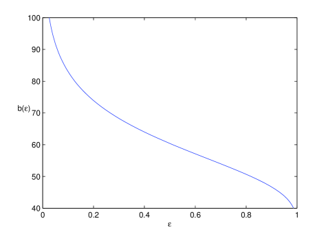
Figure 1. Dividend payout level $b$ as a function of $\varepsilon$ (Parameters: $\mu=2$, $\sigma^{2}=50$, $l=0.5$,$a=0.1$, $\delta=0.01$, $c=0.05$, $T=500$)

Example 5.2.

Let $b=100,\sigma^{2}=50,l=0.5,a=0.1,\delta=0.01,c=0.05,T=500$ the figure 2 below shows that the value function $g(x,\mu)$ increases with $(x,\mu)$, so does the company’s profit.

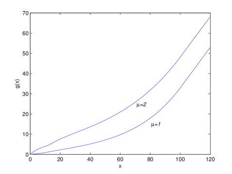
Figure 2. Value function $g(x,\mu)$ as a function of $(x,\mu)$ (Parameters: $b=100,\sigma^{2}=50,l=0.5,a=0.1,\delta=0.01,c=0.05,T=500$ )

Example 5.3.

Let $\mu=2,b=100,\sigma^{2}=50,l=0.5,a=0.5,c=0.05,T=500$. The figure 3 below shows that the value function $g(x,p)$ increases with $(x,p)$, so does the company’s profit.

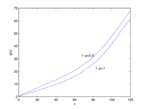
Figure 3. Value function $g(x,p)$ as a function of $(x,p)$ (Parameters: $\mu=2,b=100,\sigma^{2}=50,l=0.5,a=0.5,c=0.05,T=500$ )

Example 5.4.

Let $\mu=2,b=100,l=0.5,a=0.1,\delta=0.01,c=0.05,T=500$. The figure 4 below shows that the value function $g(x,\sigma^{2})$ increases with $(x,\sigma^{2})$, so does the company’s profit.

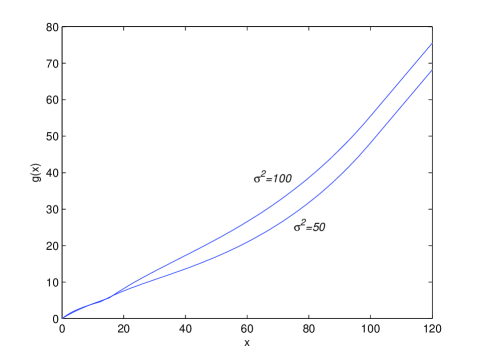
Figure 4. Value function $g(x,\sigma^{2})$ as a function of $(x,\sigma^{2})$ (Parameters: $\mu=2,b=100,l=0.5,a=0.1,\delta=0.01,c=0.05,T=500$)

Example 5.5.

Let $\mu=2,\sigma^{2}=50,l=0.5,a=0.1,\delta=0.01,c=0.05,T=500$. The figure 5 below shows that the initial capital $x(\epsilon)$ decreases with $\epsilon$.

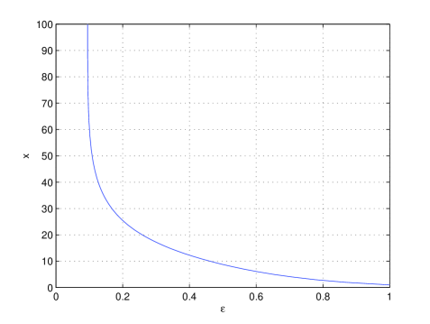
Figure 5. Initial capital $x(\epsilon)$ as a function of $\epsilon$ (Parameters: $\mu=2,\sigma^{2}=50,l=0.5,a=0.1,\delta=0.01,c=0.05,T=500$)

6. Properties on $V(x,b)$ and ruin probability

In this section, to prove Theorem 3.1, we list some lemmas on properties of $V(x,b)$ and ruin probability which will be used late. The rigorous proofs of these lemmas will be given in the appendix below. Throughout this paper we assume that $\mu/2a>1$ and $0<l\leq U(t)\leq 1$.

Lemma 6.1.

There exists $b_{0}>0$ such that if $f(x)\in C^{2}$ satisfies the following HJB equations and the boundary conditions,

$$\max\limits_{U\in[l,1]}[\frac{1}{2}\sigma^{2}U^{2}f^{{}^{\prime\prime}}(x)+(\mu U-aU^{2}-\delta)f^{{}^{\prime}}(x)-cf(x)]=0,$$ (6.1)

$$\mbox{ for}\ \ 0\leq x\leq b_{0},$$

$$f^{{}^{\prime}}(x)=1,\ \mbox{for}\ x\geq b_{0},$$

$$f^{{}^{\prime\prime}}(x)=0,\ \mbox{for}\ x\geq b_{0},$$

$$f(0)=0,$$

then we have the following,

$$\max\mathcal{L}f(x)\leq 0,f^{{}^{\prime}}(x)\geq 1,\ \mbox{ for}\ x\geq 0,$$

$$f(0)=0,$$

where $\mathcal{L}=\frac{1}{2}\sigma^{2}U^{2}\frac{d^{2}}{dx^{2}}+(\mu U-aU^{2}-\delta)\frac{d}{dx}-c$.

Lemma 6.2.

Let $b>b_{0}$ be a predetermined variable and $g\in C^{1}(R_{+})\cap C^{2}(R_{+}\setminus\{b\})$ satisfy the following HJB equations and the boundary conditions,

$$\max\limits_{U\in[l,1]}\big{[}\frac{1}{2}\sigma^{2}U^{2}g^{{}^{\prime\prime}}(x)+(\mu U-aU^{2}-\delta)g^{{}^{\prime}}(x)-cg(x)\big{]}=0,$$ (6.2)

$$\mbox{ for}\ \ 0\leq x\leq b,$$

$$g^{{}^{\prime}}(x)=1,\ \mbox{for}\ x\geq b,$$

$$g^{{}^{\prime\prime}}(x)=0,\ \mbox{for}\ x>b,$$

$$g(0)=0,$$

then we have the following,

$$\max\mathcal{L}g(x)\leq 0,\ \mbox{ for}\ x\geq 0,$$ (6.3)

$$g^{{}^{\prime}}(x)\geq 1,\ \mbox{ for}\ x\geq b,$$

$$g(0)=0,$$

where $g^{\prime\prime}(b):=g^{\prime\prime}(b-)$, $\mathcal{L}$ is defined as same as in Lemma 6.1. Indeed, the function $g(x)$ can be written as follows,

$$g(x,b)=\left\{\begin{array}[]{l l l}A\big{(}e^{\alpha_{1}x}-e^{\beta_{1}x}\big{)},&0\leq x\leq x_{1},\\ \big{(}Be^{\alpha_{2}x_{2}}+Ce^{\beta_{2}x_{2}}\big{)}\exp\big{\{}-\int_{x}^{x_{2}}\frac{c}{\frac{1}{2}\mu\eta(y)-\delta}dy\big{\}},&x_{1}<x<x_{2},\\ Be^{\alpha_{2}x}+Ce^{\beta_{2}x},&x_{2}\leq x\leq b,\\ x-b+Be^{\alpha_{2}b}+Ce^{\beta_{2}b},&x>b,\end{array}\right.$$ (6.8)

where

$$\alpha_{1}=\frac{-(\mu l-al^{2}-\delta)+\sqrt{(\mu l-al^{2}-\delta)^{2}+2c\sigma^{2}l^{2}}}{\sigma^{2}l^{2}},$$ (6.9)

$$\beta_{1}=\frac{-(\mu l-al^{2}-\delta)-\sqrt{(\mu l-al^{2}-\delta)^{2}+2c\sigma^{2}l^{2}}}{\sigma^{2}l^{2}},$$ (6.10)

$$\alpha_{2}=\frac{-(\mu-a-\delta)+\sqrt{(\mu-a-\delta)^{2}+2c\sigma^{2}}}{\sigma^{2}},$$ (6.11)

$$\beta_{2}=\frac{-(\mu-a-\delta)-\sqrt{(\mu-a-\delta)^{2}+2c\sigma^{2}}}{\sigma^{2}}$$ (6.12)

$$A=\frac{Be^{\alpha_{2}x_{2}}+Ce^{\beta_{2}x_{2}}}{e^{\alpha_{1}x_{1}}-e^{\beta_{1}x_{1}}}\exp\big{\{}-\int_{x_{1}}^{x_{2}}\frac{c}{\frac{1}{2}\mu\eta(y)-\delta}dy\big{\}},$$ (6.13)

$$B=\frac{[-c+(\frac{1}{2}\mu 1-\delta)\beta_{2}]e^{\beta_{2}x_{2}}}{[-c+(\frac{1}{2}\mu 1-\delta)\beta_{2}]e^{\beta_{2}x_{2}+\alpha_{2}b}\alpha_{2}-[-c+(\frac{1}{2}\mu 1-\delta)\alpha_{2}]e^{\alpha_{2}x_{2}+\beta_{2}b}\beta_{2}},$$

$$C=\frac{[-c+(\frac{1}{2}\mu 1-\delta)\alpha_{2}]e^{\alpha_{2}x_{2}}}{-[-c+(\frac{1}{2}\mu 1-\delta)\beta_{2}]e^{\beta_{2}x_{2}+\alpha_{2}b}\alpha_{2}+[-c+(\frac{1}{2}\mu 1-\delta)\alpha_{2}]e^{\alpha_{2}x_{2}+\beta_{2}b}\beta_{2}},$$ (6.15)

$$x_{1}=\frac{1}{\alpha_{1}-\beta_{1}}\log\big{[}\frac{c-\beta_{1}(\frac{1}{2}\mu l-\delta)}{c-\alpha_{1}(\frac{1}{2}\mu l-\delta)}\big{]}>0,$$ (6.16)

$$x_{2}=x_{1}+\frac{\sigma^{2}}{2a}\big{[}\frac{G}{G-H}\log(\frac{G-l}{G-1})-\frac{H}{G-H}\log(\frac{l-H}{1-H})\big{]},$$ (6.17)

$$G = \frac{2c\sigma^{2}+\mu^{2}+4a\delta+\sqrt{(2c\sigma^{2}+\mu^{2}+4a\delta)^{2}-16a\mu^{2}\delta}}{4a\mu},$$ (6.18)

$$H = \frac{2c\sigma^{2}+\mu^{2}+4a\delta-\sqrt{(2c\sigma^{2}+\mu^{2}+4a\delta)^{2}-16a\mu^{2}\delta}}{4a\mu},$$ (6.19)

$$K = (G-l)^{G/(G-H)}(l-H)^{-H/(G-H)},$$ (6.20)

and $\eta(x)$ is uniquely determined by

$$[G-\eta(x)]^{G/(G-H)}[\eta(x)-H]^{-H/(G-H)}=K\exp\big{[}-\frac{2a}{\sigma^{2}}(x-x_{1})\big{]}.$$ (6.21)

Lemma 6.3.

Let $g(b,x)$ be as the same as in lemma 6.2. Then $\frac{\partial}{\partial b}g(b,x)\leq 0$ holds for $b\geq b_{0}$.

Lemma 6.4.

The ruin probability $\mathbf{P}[\tau_{b}^{b}\leq T]$ is strictly increasing w.r.t. $b$ on $[x_{2},b_{K})$, where $b_{K}:=\inf\{b:\mathbf{P}[\tau_{b}^{b}\leq T]=0\}$, and $x_{2}$ is defined by (6.17), $\tau^{b}_{b}:=\tau_{b}^{\pi_{b}^{*}}$.

Lemma 6.5.

Let $\phi^{b}(t,y)\in C^{1}(0,\infty)\cap C^{2}(0,b)$ and satisfy the following partial differential equation and the boundary conditions,

$$\left\{\begin{array}[]{l l l}\phi_{t}^{b}(t,y)=\frac{1}{2}[U_{b}^{*}(y)]^{2}\sigma^{2}\phi_{yy}^{b}(t,y)+(\mu U_{b}^{*}(y)-a[U_{b}^{*}(y)]^{2}-\delta)\phi_{y}^{b}(t,y),\\ \phi^{b}(0,y)=1,\ \mbox{for}\ \ 0<y\leq b,\\ \phi^{b}(t,0)=0,\phi_{y}^{b}(t,y)=0,\ \mbox{for}\ t>0.\end{array}\right.$$ (6.25)

Then $\phi^{b}(T,y)=1-\psi^{b}(T,y)$, where $\psi^{b}(T,y):={\bf P}\big{\{}\tau_{y}^{b}<T\big{\}}$, and $U^{*}(x)$ is defined by

$$U^{*}_{b}(x)=\left\{\begin{array}[]{l l l}l,&0\leq x\leq x_{1},\\ \eta(x)&x_{1}<x<x_{2},\\ 1,&x_{2}\leq x.\end{array}\right.$$ (6.29)

Lemma 6.6.

Let the function $\phi^{b}(t,x)$ solve the equation(6.25) and $u(b)\equiv\phi^{b}(T,b)$. Then $u(b)$ is a continuous function of $b$ on $[b_{0},+\infty)$.

7. Proof of Main Result

In this section we will give the proof of Theorem 3.1. Before this proof we first prove the following.

Theorem 7.1.

Let $f(x)$, $g(x,b)$ and $U^{*}_{b}(x)$ be as the same as in lemma 6.1, lemma 6.2 and lemma 6.5,respectively.    Then
(i) If $b\leq b_{0}$ we have $V(x,b)=V(x,b_{0})=V(x)=f(x)$, the optimal strategy associated with $V(x)$ is $\pi_{b_{o}}^{\ast}=\{U^{*}_{b_{0}}(R^{\pi_{b_{o}}^{\ast}}_{\cdot}),L^{\pi_{b_{o}}^{\ast}}_{\cdot}\}$, where the process $\{R^{\pi_{b_{o}}^{\ast}}_{t},L^{\pi_{b_{o}}^{\ast}}_{t}\}$ is uniquely determined by the following SDE,

$$\left\{\begin{array}[]{l l l}dR_{t}^{\pi_{b_{o}}^{\ast}}=(\mu U^{*}_{b_{0}}(R^{\pi_{b_{o}}^{\ast}}_{t})-a{U^{*}_{b_{0}}}^{2}(R^{\pi_{b_{o}}^{\ast}}_{t})-\delta)dt+\sigma U^{*}_{b_{0}}(R^{\pi_{b_{o}}^{\ast}}_{t})d{W}_{t}-dL_{t}^{\pi_{b_{o}}^{\ast}},\\ R_{0}^{\pi_{b_{o}}^{\ast}}=x,\\ 0\leq R^{\pi_{b_{o}}^{\ast}}_{t}\leq b_{0},\\ \int^{\infty}_{0}I_{\{t:R^{\pi_{b_{o}}^{\ast}}_{t}<b_{0}\}}(t)dL_{t}^{\pi_{b_{o}}^{\ast}}=0.\end{array}\right.$$ (7.5)

(ii) If $b>b_{0}$ we have $V(x,b)=g(x)$ and the optimal strategy $\pi_{b^{*}}^{\ast}$ is $\{U^{\ast}_{b^{*}}(R^{\pi_{b^{*}}^{\ast}}_{t}),L^{\pi_{b^{*}}^{\ast}}_{t}\}$, where $\{R^{\pi_{b^{*}}^{\ast}}_{t},L^{\pi_{b^{*}}^{\ast}}_{t}\}$ is uniquely determined by the following SDE

$$\left\{\begin{array}[]{l l l}dR_{t}^{\pi_{b^{*}}^{\ast}}=(\mu U^{*}_{b^{*}}(R^{\pi_{b^{*}}^{\ast}}_{t})-a{U^{*}_{b^{*}}}^{2}(R^{\pi_{b^{*}}^{\ast}}_{t})-\delta)dt+\sigma U^{*}_{b^{*}}(R^{\pi_{b^{*}}^{\ast}}_{t})d{W}_{t}-dL_{t}^{\pi_{b^{*}}^{\ast}},\\ R_{0}^{\pi_{b^{*}}^{\ast}}=x,\\ 0\leq R^{\pi_{b^{*}}^{\ast}}_{t}\leq b^{*},\\ \int^{\infty}_{0}I_{\{t:R^{\pi_{b^{*}}^{\ast}}_{t}<b^{*}\}}(t)dL_{t}^{\pi_{b^{*}}^{\ast}}=0.\end{array}\right.$$ (7.10)

Proof.

(i) If $b\leq b_{0}$ then since $\pi^{*}_{b_{0}}\in\Pi_{b_{0}}\subset\Pi_{b}$ we have $V(x,b_{0})\leq V(x,b)\leq V(x)$. It suffices to show $V(x)\leq f(x)=V(x,b_{0})$. For a admissible strategy $\pi=\{a_{\pi},L^{\pi}\}$ we assume that $(R^{\pi}_{t},L^{\pi}_{t})$ is the process defined by (2.4). Set $\Lambda=\{s:L_{s-}^{\pi}\neq L_{s}^{\pi}\}$ and let $\hat{L}=\sum_{s\in\Lambda,s\leq t}(L_{s}^{\pi}-L_{s-}^{\pi})$ and $\tilde{L}_{t}^{\pi}=L_{t}^{\pi}-\hat{L}_{t}^{\pi}$ denote the discontinuous part and continuous part of $L_{s}^{\pi}$,respectively. Let $\tau^{\varepsilon}=\inf\{t\geq 0:R^{\pi}_{t}\leq\varepsilon\}$. Applying Itô formula to stochastic process $R^{\pi}_{t}$ and $f(x)$, we have

$$e^{-c(t\wedge\tau^{\varepsilon})}f(R_{t\wedge\tau^{\varepsilon}}^{\pi}) = f(x)+\int_{0}^{t\wedge\tau^{\varepsilon}}e^{-cs}\mathcal{L}f(R_{s}^{\pi})ds$$ (7.11)

$$+ \int_{0}^{t\wedge\tau^{\varepsilon}}a_{\pi}\sigma e^{-cs}f^{{}^{\prime}}(R_{s}^{\pi})d\mathcal{W}_{s}\mathcal{-}\int_{0}^{t\wedge\tau^{\varepsilon}}e^{-cs}f^{{}^{\prime}}(R_{s}^{\pi})dL_{s}^{\pi}$$

$$+ \sum\limits_{s\in\Lambda,s\leq t\wedge\tau^{\varepsilon}}e^{-cs}[f(R_{s}^{\pi})-f(R_{s-}^{\pi})$$

$$- f^{{}^{\prime}}(R_{s-}^{\pi})(R_{s}^{\pi}-R_{s-}^{\pi})]$$

$$= f(x)+\int_{0}^{t\wedge\tau^{\varepsilon}}e^{-cs}\mathcal{L}f(R_{s}^{\pi})ds$$

$$+ \int_{0}^{t\wedge\tau^{\varepsilon}}a_{\pi}\sigma e^{-cs}f^{{}^{\prime}}(R_{s}^{\pi})d\mathcal{W}_{s}\mathcal{-}\int_{0}^{t\wedge\tau^{\varepsilon}}e^{-cs}f^{{}^{\prime}}(R_{s}^{\pi})d\tilde{L}_{s}^{\pi}$$

$$+ \sum\limits_{s\in\Lambda,s\leq t\wedge\tau^{\varepsilon}}e^{-cs}[f(R_{s}^{\pi})-f(R_{s-}^{\pi}))],$$

where

$$\mathcal{L}=\frac{1}{2}U^{2}\sigma^{2}\frac{d^{2}}{dx^{2}}+(\mu U-aU^{2}-\delta)\frac{d}{dx}-c.$$

By lemma 6.1 the second term in the right-hand side of last equation is nonpositive. Since $f^{{}^{\prime}}(R_{s\wedge\tau^{\varepsilon}}^{\pi})\leq f^{{}^{\prime}}(\varepsilon)$, the third term is a square integrable martingale. Taking expectations on both sides of Eq.(7.11) and then letting $\varepsilon\rightarrow 0$ one has

$${\bf E}\big{\{}e^{-c(t\wedge\tau^{\pi}_{x})}f(R_{t\wedge\tau^{\pi}_{x}}^{\pi})\big{\}} \leq f(x)-{\bf E}\big{\{}\int_{0}^{t\wedge\tau^{\pi}_{x}}e^{-cs}f^{{}^{\prime}}(R_{s}^{\pi})d\tilde{L}_{s}^{\pi}\big{\}}$$

$$+ {\bf E}\big{\{}\sum\limits_{s\in\Lambda,s\leq t\wedge\tau^{\pi}_{x}}e^{-cs}[f(R_{s}^{\pi})-f(R_{s-}^{\pi})]\big{\}}.$$

Since $f^{{}^{\prime}}(x)\geq 1$ for $x\geq 0$,

$$f(R_{s}^{\pi})-f(R_{s-}^{\pi})\leq-(L_{s}^{\pi}-L_{s-}^{\pi}).$$ (7.13)

So the inequalities (7) and (7.13) yield

$${\bf E}\big{\{}e^{-c(t\wedge\tau^{\pi}_{x})}f(R_{t\wedge\tau^{\pi}_{x}}^{\pi})\big{\}} + {\bf E}\big{\{}\int_{0}^{t\wedge\tau^{\pi}_{x}}e^{-cs}dL_{s}^{\pi}\big{\}}\leq f(x).$$ (7.14)

By the definition of $\tau^{\pi}_{x}$ ,$f(0)=0$ and $f^{\prime}(x)\geq 1$, it easily follows that

$$\liminf\limits_{t\rightarrow\infty}e^{-c(t\wedge\tau^{\pi}_{x})}f(R_{t\wedge\tau^{\pi}_{x}}^{\pi}) = e^{-c\tau}f(0)I_{\{\tau^{\pi}_{x}<\infty\}}$$ (7.15)

$$+ \liminf\limits_{t\rightarrow\infty}e^{-ct}f(R_{t})I_{\{\tau^{\pi}_{x}=\infty\}}\geq 0.$$

So we deduce from the inequalities ( 7.14 ) and (7.15 ) that

$$J(x,\pi)={\bf E}[\big{\{}\int_{0}^{\tau^{\pi}_{x}}e^{-cs}dL_{s}^{\pi}\}]\leq f(x).$$

Therefore

$$V(x)\leq f(x).$$

If we choose the control strategy $\pi_{b_{o}}^{\ast}=\{U^{*}_{b_{0}}(R^{\pi_{b_{o}}^{\ast}}_{\cdot}),L^{\pi_{b_{o}}^{\ast}}_{\cdot}\}$ and stochastic process $(R^{\pi_{b_{o}}^{\ast}}_{t},L^{\pi_{b_{o}}^{\ast}}_{t})$ as in SDE (7.5, the inequalities above become equalities, so

$$V(x)\leq f(x)=V(x,b_{0}).$$

(i) thus follows. (ii) Assume $b\geq b_{0}$. Let $(R^{\pi}_{t},L^{\pi}_{t})$ be the process as in (2.4) for $\pi\in\Pi_{b}$. Then

$$\left\{\begin{array}[]{l l l}\mathbf{P}\{R_{s-}^{\pi}\geq R_{s}^{\pi}\geq b\}+\mathbf{P}\{b\geq R_{s-}^{\pi}\geq R_{s}^{\pi}\}=1,\ \forall s\geq 0,\\ \mathcal{L}g(R_{s}^{\pi})\leq 0\ \mbox{ $s\leq\tau^{\pi}_{x}=\inf\{t\geq 0:R^{\pi}_{s}\leq 0\}$},\\ g^{\prime}(x)=1\ \mbox{ $x\geq b$}.\end{array}\right.$$ (7.19)

Replacing $f$ in proof of (i) above with $g$, then using (7.19) and the same argument as in (i) we can get

$$V(x,b)\leq g(x).$$

Similarly, letting $\pi_{b}^{\ast}=\{U^{*}_{b}(R^{\pi_{b}^{\ast}}_{\cdot}),L^{\pi_{b}^{\ast}}_{\cdot}\}$ we derive $V(x,b)=g(x)$. Therefore (ii) follows. ∎

Now we turn to proof of Theorem 3.1. Proof of Theorem 3.1. If $\mathbf{P}[\tau_{b_{0}}^{\pi^{*}_{b_{0}}}\leq T]\leq\varepsilon$, then the conclusion is obvious because the constraints does not work and the proof reduces to the usual optimal control problem. If $\mathbf{P}[\tau_{b_{0}}^{\pi^{*}_{b_{0}}}\leq T]>\varepsilon$, then by lemmas 6.4-6.6 there exists a unique $b^{\ast}$ solving equation $\mathbf{P}\{\tau_{b}^{\pi^{*}_{b}}\leq T\}=\varepsilon$ and $x_{2}<b^{\ast}=\inf\{b:b\in\mathfrak{B}\}>b_{0}$. By theorem 7.1 we know that $b^{\ast}$ meets (3.6) and (3.7) because $V(x,b)=g(x,b)$ is a decreasing function of $b(\geq b_{0})\in[x_{2},b_{K})$ due to lemma 6.3. So the optimal strategy associated with the optimal return function $V(x,b^{*})=g(x,b^{*})$ is $\{U^{\ast}_{b^{*}}(R^{\pi_{b^{*}}^{\ast}}_{t}),L^{\pi_{b^{*}}^{\ast}}_{t}\}$ and $\{R^{\pi_{b^{*}}^{\ast}}_{t},L^{\pi_{b^{*}}^{\ast}}_{t}\}$ is uniquely determined by SDE (3.12). Thus we complete the proof.   $\Box$

8. Appendix

In this section we will give the proofs of lemmas we concerned with throughout this paper. Proof of lemma 6.1.  Since the proof is complete similar to that of Guo Xin, Liu Jun and Zhou Xunyu[11](2004), we omit it here. Proof of lemma 6.2.  Since the proof is somewhat similar to that of He, Hou and Liang [13](2008) and Guo, Liu and Zhou [11](2004), we only give the sketch of the proof as follows.
If the $\max$ in (6.2) is attained in the interior of the control region, then, by differentiating w.r.t. $U$, we can find the maximizing function $U^{*}_{b}(x)$ can be defined by (6.29) above, and

$$\eta(x)=\frac{\mu g^{\prime}(x)}{2ag^{\prime}(x)-\sigma^{2}g^{\prime\prime}(x)}=\frac{2cg(x)}{\mu g^{\prime}(x)}+\frac{2\delta}{\mu},0\leq x\leq b.$$ (8.1)

Letting $x\rightarrow 0+$ we have $\eta(x)\rightarrow 2\delta/\mu<l$, whereas taking $x\rightarrow b_{0}$ and noticing that $g^{\prime\prime}(b_{0})=0$, we also have $\eta(x)\rightarrow\mu/2a>1$. So by (6.29) we find $0\leq x_{1}<x_{2}\leq b_{0}<b$ such that

$$U^{*}(x)=\left\{\begin{array}[]{l l l}l,&0\leq x\leq x_{1},\\ \eta(x)&x_{1}<x<x_{2},\\ 1,&x_{2}\leq x\leq b.\end{array}\right.$$ (8.5)

Putting this expression into (6.2) we have (6.8). Then by smooth fit principle we can determine parameters $\alpha_{1}$, $\beta_{1}$,$\alpha_{2}$, $\beta_{2}$, $x_{1}$, $x_{2}$, $A$, $B$, $C$, $G$,$H$ and $K$ by (6.9)-(6.18). Now it remains to prove the solution $g$ defined by (6.8) satisfies (6.3). We only need to prove

$$\max\limits_{U\in[l,1]}[\frac{1}{2}\sigma^{2}U^{2}g^{{}^{\prime\prime}}(x)+(\mu U-aU^{2}-\delta)g^{{}^{\prime}}(x)-cg(x)]=0,\ \mbox{ for}\ x\geq b.$$

For $x\geq b$, we first prove $g^{\prime\prime}(b-)\geq 0$. Noticing that

$$g^{\prime\prime}(b-)=\frac{\alpha_{2}^{2}v(\beta_{2})e^{\beta_{2}x_{2}+\alpha_{2}b}-\beta_{2}^{2}v(\alpha_{2})e^{\alpha_{2}x_{2}+\beta_{2}b}}{v(\beta_{2})e^{\beta_{2}x_{2}+\alpha_{2}b}\alpha_{2}-v(\alpha_{2})e^{\alpha_{2}x_{2}+\beta_{2}b}\beta_{2}},$$

where $v(t)\equiv-c+(\frac{1}{2}\mu-\delta)t$. Since $|\alpha_{2}|\leq|\beta_{2}|$, $v(\beta_{2})<v(\alpha_{2})<0$, $\alpha_{2}>0,\beta_{2}<0$ and $g^{\prime\prime}(b_{0})=0$, the numerator and denominator of (8) are strictly negative, so $g^{\prime\prime}(b-)\geq 0$ . Then by (6.2)

$$\max\mathcal{L}\{g(x)\} = (\mu-a-\delta)-c(x-b+g(b))$$

$$\leq \mu-a-\delta-cg(b)$$

$$\leq \frac{1}{2}\sigma^{2}a^{2}g^{\prime\prime}(b-)+\mu-a-\delta-cg(b)\leq 0.$$

Thus we complete the proof.

Proof of lemma 6.3. If $x\geq b$, then using (6.8) and $g^{\prime}(x)=1$ one has

$$\frac{\partial}{\partial b}g(b,x) = -1+\alpha_{2}Be^{\alpha_{2}b}+\beta_{2}Ce^{\beta_{2}b}+B^{\prime}e^{\alpha_{2}b}+C^{\prime}e^{\beta_{2}b}$$ (8.7)

$$= B^{\prime}e^{\alpha_{2}b}+C^{\prime}e^{\beta_{2}b}$$

where $B^{\prime}$ and $C^{\prime}$ denote derivatives w.r.t $b$ of $B$ and $C$,respectively. By the first three expressions in (6.8) the proof reduces to showing that for $x_{2}\leq x\leq b$

$$B^{\prime}e^{\alpha_{2}x}+C^{\prime}e^{\beta_{2}x}\leq 0.$$ (8.8)

By (6.18)-(6.21) one has

$$B^{\prime}e^{\alpha_{2}x}+C^{\prime}e^{\beta_{2}x} = \big{\{}\frac{[v(\alpha_{2})e^{\alpha_{2}x_{2}+\beta_{2}x}-v(\beta_{2})e^{\beta_{2}x_{2}+\alpha_{2}x}]}{[\alpha_{2}v(\beta_{2})e^{\beta_{2}x_{2}+\alpha_{2}b}-\beta_{2}v(\alpha_{2})e^{\alpha_{2}x_{2}+\beta_{2}b}]^{2}}\big{\}}$$

$$\times\big{[}\alpha_{2}^{2}v(\beta_{2})e^{\beta_{2}x_{2}+\alpha_{2}b}-\beta_{2}^{2}v(\alpha_{2})e^{\alpha_{2}x_{2}+\beta_{2}b}\big{]}$$

$$= \frac{K_{1}(x)}{K_{2}^{2}(x_{2})}\times K_{3}(b).$$

where

$$K_{1}(x) = v(\alpha_{2})e^{\alpha_{2}x_{2}+\beta_{2}x}-v(\beta_{2})e^{\beta_{2}x_{2}+\alpha_{2}x},$$

$$K_{2}(x) = \alpha_{2}v(\beta_{2})e^{\beta_{2}x+\alpha_{2}b}-\beta_{2}v(\alpha_{2})e^{\alpha_{2}x+\beta_{2}b},$$

$$K_{3}(x) = \alpha_{2}^{2}v(\beta_{2})e^{\beta_{2}x_{2}+\alpha_{2}x}-\beta_{2}^{2}v(\alpha_{2})e^{\alpha_{2}x_{2}+\beta_{2}x}.$$

Since $K_{1}(x)$ is an increasing function of $x$ and $K_{1}(x_{2})>0$, $K_{1}(x)>0$ for $x\in[x_{2},b]$. Noting that $K_{3}(b)\leq 0$, we know that (8.8) is true.    $\Box$

Proof of lemma 6.4.  Because the proof of decreasing property is complete similar to that of theorem 3.1 in [13](2008), we only need to prove that the probability of bankruptcy is strictly decreasing on $[x_{2},b_{K}]$, that is,

$$\mathbf{P}[\tau_{b_{1}}^{b_{1}}\leq T]-\mathbf{P}[\tau_{b_{2}}^{b_{2}}\leq T]>0$$

for any $b_{2}>b_{1}\geq x_{2}$. By comparison theorem,

$$\mathbf{P}[\tau_{b_{1}}^{b_{1}}\leq T]-\mathbf{P}[\tau_{b_{2}}^{b_{2}}\leq T]\geq\mathbf{P}[\tau_{b_{1}}^{b_{2}}\leq T]-\mathbf{P}[\tau_{b_{2}}^{b_{2}}\leq T].$$

The proof can be reduced to proving that

$$\mathbf{P}[\tau_{b_{1}}^{b_{2}}\leq T]-\mathbf{P}[\tau_{b_{2}}^{b_{2}}\leq T]>0.$$ (8.9)

To prove the inequality (8.9) we define stochastic processes $R_{t}^{[1]}$ and $R_{t}^{[2]}$ by the following SDEs:

$$dR_{t}^{[1]}=[\mu U_{b_{2}}^{*}(R_{t}^{[1]})-a{U_{b_{2}}^{*}}^{2}(R_{t}^{[1]})-\delta]dt+U_{b_{2}}^{*}(R_{t}^{[1]})\sigma d\mathcal{W}_{t}-dL_{t}^{b_{2}},R_{0}^{[1]}=b_{1},$$

$$dR_{t}^{[2]}=[\mu U_{b_{2}}^{*}(R_{t}^{[2]})-a{U_{b_{2}}^{*}}^{2}(R_{t}^{[2]})-\delta]dt+U_{b_{2}}^{*}(R_{t}^{[2]})\sigma d\mathcal{W}_{t}-dL_{t}^{b_{2}},R_{0}^{[2]}=b_{2},$$

respectively, where $U_{b}^{*}(\cdot)$ is as in (6.29). Let $\tau^{b_{1}}=\inf\limits_{t\geq 0}\{t:R_{t}^{[2]}=b_{1}\}$, $A=\{\tau^{b_{1}}\leq T\}$ and $B=\big{\{}\sl R_{t}^{[2]}$ will go to bankruptcy in a time interval $[\tau^{b_{1}},\tau^{b_{1}}+T]$ and $\tau^{b_{1}}\leq T\big{\}}$. Then $\{\tau_{b_{2}}^{b_{2}}\leq T\}\subset B\subset A$. Moreover, by using strong Markov property of $R_{t}^{[2]}$, we have

$$\mathbf{P}[\tau_{b_{1}}^{b_{2}}\leq T]=\mathbf{P}[B|A].$$

So

$$\mathbf{P}[\tau_{b_{1}}^{b_{2}}\leq T]-\mathbf{P}[\tau_{b_{2}}^{b_{2}}\leq T] \geq \mathbf{P}[\tau_{b_{1}}^{b_{2}}\leq T]-\mathbf{P}(B)$$

$$= \mathbf{P}[\tau_{b_{1}}^{b_{2}}\leq T]-\mathbf{P}(A)\mathbf{P}(B|A)$$

$$= \mathbf{P}[\tau_{b_{1}}^{b_{2}}\leq T](1-\mathbf{P}(A))$$

$$= \mathbf{P}[\tau_{b_{1}}^{b_{2}}\leq T]\mathbf{P}(A^{c}).$$

By theorem 4.1, $\mathbf{P}[\tau_{b_{1}}^{b_{2}}\leq T]\geq\mathbf{P}[\tau_{b_{1}}^{b_{1}}\leq T]>0$. So we only need to prove $\mathbf{P}(A^{c})>0$. For doing this we define stochastic processes $R_{t}^{[3]}$ and $R_{t}^{[4]}$ by the following SDEs

$$\left\{\begin{array}[]{l l l}dR_{t}^{[3]}=[\mu U_{b_{2}}^{*}(R_{t}^{[3]})-a{U_{b_{2}}^{*}}^{2}(R_{t}^{[3]})-\delta]dt+U_{b_{2}}^{*}(R_{t}^{[3]})\sigma d\mathcal{W}_{t}-dL_{t}^{b_{2}},\\ R_{0}^{[3]}=\frac{b_{1}+b_{2}}{2}\end{array}\right.$$

and

$$\left\{\begin{array}[]{l l l}dR_{t}^{[4]}=[\mu U_{b_{2}}^{*}(R_{t}^{[4]})-a{U_{b_{2}}^{*}}^{2}(R_{t}^{[4]})-\delta]dt+U_{b_{2}}^{*}(R_{t}^{[4]})\sigma d\mathcal{W}_{t},\\ R_{0}^{[4]}=\frac{b_{1}+b_{2}}{2}.\end{array}\right.$$

Setting $D=\{\inf\limits_{0\leq t\leq T}R_{t}^{[3]}>b_{1}\}$ and $E=\{\inf\limits_{0\leq t\leq T}R_{t}^{[4]}>b_{1},\sup\limits_{0\leq t\leq T}R_{t}^{[4]}<b_{2}\}$, by comparison theorem on SDE, we have $\mathbf{P}(A^{c})\geq\mathbf{P}(D)\geq\mathbf{P}(E)$. Since $U_{b_{2}}^{*}(x)=1$ we have

$$R_{t}^{[4]}=\frac{b_{1}+b_{2}}{2}+[\mu-a-\delta]t+\sigma\mathcal{W}_{t}\ \mbox{ on $E$}.$$ (8.12)

We deduce from (8.12) and properties of Brownian motion with drift (cf. Borodin and Salminen [1] (2002)) that

$$\mathbf{P}(E)=\frac{e^{-\mu^{\prime 2}T/2}}{\sqrt{2\pi T}}\sum_{k=-\infty}^{\infty}\int_{b_{1}/\sigma}^{b_{2}/\sigma}e^{\mu^{\prime}(z-x)}[(e^{-(z-x+\frac{2k(b_{2}-b_{1})}{\sigma})^{2}/2T})$$

$$-(e^{-(z+x-\frac{2b_{1}-2k(b_{2}-b_{1})}{\sigma})^{2}/2T})]dz>0,$$

where $\mu^{\prime}=(\mu-a-\delta)/\sigma$ and $x=\frac{b_{1}+b_{2}}{2\sigma}$. Thus the proof follows. $\Box$ Proof of lemma 6.5. Let $\phi(t,y)\equiv\phi^{b}(t,y)$. Since the stochastic process $(R^{\pi_{b}^{\ast},y}_{t\wedge\tau_{y}^{b}},L_{t\wedge\tau_{y}^{b}}^{\pi_{b}^{\ast}})$ is continuous, by applying the generalized Itô formula to $(R^{\pi_{b}^{\ast},y}_{t\wedge\tau_{y}^{b}},L_{t\wedge\tau_{y}^{b}}^{\pi_{b}^{\ast}})$ and $\phi(t,y)$, we have for $0<y\leq b$

$$\phi(T-(t\wedge\tau_{y}^{b}),Y_{t\wedge\tau_{y}^{b}}^{b}) = \phi(T,y)$$ (8.13)

$$+ \int_{0}^{t\wedge\tau_{y}^{b}}(\frac{1}{2}U^{*2}(Y_{s}^{b})\sigma^{2}\phi_{yy}(T-s,Y_{s}^{b})$$

$$+ (\mu U^{*}(Y_{s}^{b})-a[U^{*}((Y_{s}^{b}))]^{2}-\delta)\phi_{y}(T-s,Y_{s}^{b})$$

$$- \phi_{t}(T-s,Y_{s}^{b}))ds-\int_{0}^{t\wedge\tau_{y}^{b}}\phi_{y}(T-s,Y_{s}^{b})dL_{s}^{b}$$

$$+ \int_{0}^{t\wedge\tau_{y}^{b}}a(Y_{s}^{b})\sigma\phi_{y}(T-s,Y_{s}^{b})dW_{s}^{b}.$$

where $\tau_{y}^{b}\equiv\tau^{\pi_{b}^{\ast}}_{y}=\inf\{t:R^{\pi_{b}^{\ast},y}_{t}=0\}$.
Letting $t=T$ and taking mathematical expectation at both sides of (8.13) yield that

$$\phi(T,y) = \mathbf{E}[\phi(T-(T\wedge\tau_{y}^{b}),R^{\pi_{b}^{\ast},y}_{T\wedge\tau_{y}^{b}})]$$

$$= \mathbf{E}[\phi(0,R^{\pi_{b}^{\ast},y}_{T})1_{T<\tau_{y}^{b}}]+\mathbf{E}[\phi(T-\tau_{y}^{b},0)1_{T\geq\tau_{y}^{b}})]$$

$$= \mathbf{E}[1_{T<\tau_{y}^{b}}]=1-\psi(T,y).$$

$\Box$ Proof of lemma 6.6. Let $a(y):=\frac{1}{2}[U_{b}^{*}(y)]^{2}\sigma^{2}$ $\mu(y):=\mu U_{b}^{*}(y)-a[U_{b}^{*}(y)]^{2}-\delta$. Then the equation (6.25) becomes

$$\phi_{t}^{b}(t,y)=a(y)\phi_{yy}^{b}(t,y)+\mu(y)\phi_{y}^{b}(t,y).$$ (8.14)

By the properties of $U_{b}^{*}(y)$, we can easily show that $a(y)$ and $\mu(y)$ are continuous in $[0,b]$. So there exists a unique solution in $C^{1}(0,\infty)\cap C^{2}(0,b)$ for (6.25). Moreover, $a^{{}^{\prime}}(y)$, $\mu^{{}^{\prime}}(y)$ and $a^{{}^{\prime\prime}}(y)$ are bounded in $(0,x_{1})$,$(x_{1},x_{2})$ and $(x_{2},b)$. So we only need to prove that $\phi^{b}(t,x)$ is continuous in $b$. Let $y=bz$ and $\theta^{b}(t,z)=\phi^{b}(t,by)$, the equation (6.25) becomes

$$\left\{\begin{array}[]{l l l}\theta_{t}^{b}(t,z)=[a(bz)/b^{2}]\theta_{zz}^{b}(t,z)+[\mu(bz)/b]\theta_{z}^{b}(t,z),\\ \theta^{b}(0,z)=1,\ \mbox{for}\ 0<z\leq 1,\\ \theta^{b}(t,0)=0,\theta_{z}^{b}(t,1)=0,\ \mbox{for}\ t>0.\end{array}\right.$$ (8.18)

So the proof of Lemma 6.6 reduces to proving $\lim\limits_{b_{2}\rightarrow b_{1}}\theta^{b_{2}}(t,z)=\theta^{b_{1}}(t,z)$ for fixed $b_{1}>b_{0}$. Setting $w(t,z)=\theta^{b_{2}}(t,z)-\theta^{b_{1}}(t,z)$, we have

$$\left\{\begin{array}[]{l l l}w_{t}(t,z)&=&[a(b_{2}z)/b_{2}^{2}]w_{zz}(t,z)+[\mu(b_{2}z)/b_{2}]w_{z}(t,z)\\ &+&\{a(b_{2}z)/b_{2}^{2}-a(b_{1}z)/b_{1}^{2}\}\theta_{zz}^{b_{1}}(t,z)\\ &+&\{a(b_{2}z)/b_{2}^{2}-a(b_{1}z)/b_{1}^{2}\}\theta_{z}^{b_{1}}(t,z),\\ w(0,z)&=&0,\ \mbox{for}\ 0<z\leq 1,\\ w(t,0)&=&0,\ w_{x}(t,1)=0,\ \mbox{for}\ t>0.\end{array}\right.$$ (8.24)

By multiplying the first equation in (8.24) by $w(t,z)$ and then integrating on $[0,t]\times[0,1]$,

$$\int_{0}^{t}\int_{0}^{1}w(s,x)w_{t}(s,x)dxds$$ (8.25)

$$= \int_{0}^{t}\int_{0}^{1}\big{\{}[a(b_{2}x)/b_{2}^{2}]w(s,x)w_{xx}(s,x)$$

$$+ [\mu(b_{2}x)/b_{2}]w(s,x)w_{x}(s,x)$$

$$+ [a(b_{2}x)/b_{2}^{2}-a(b_{1}x)/b_{1}^{2}]w(s,x)\theta_{xx}^{b_{1}}(t,x)$$

$$+ w(s,x)[\mu(b_{2}x)/b_{2}-\mu(b_{1}x)/b_{1}]w(s,x)\theta_{x}^{b_{1}}(t,x)\big{\}}dxds$$

$$\equiv E_{1}+E_{2}+E_{3}+E_{4}.$$

We now estimate terms $E_{i}$, $i=1,\cdots,4$, as follows. By definitions of $a(x)$ and $\mu(x)$, there exit positive constants $D_{1}$, $D_{2}$ and $D_{3}$ such that $[\mu(b_{2}z)/b_{2}]^{2}\leq D_{1}$, $[a(bx)/b^{2}]^{\prime}\geq 0$, $[a(b_{2}x)/b_{2}^{2}]\geq D_{2}$ and $[a(b_{2}x)/b_{2}^{2}]^{\prime}\leq D_{3}$, so by Young’s inequality, we have for any $\lambda_{1}>0$ and $\lambda_{2}>0$

$$E_{1} = \int_{0}^{t}\int_{0}^{1}[a(b_{2}x)/b_{2}^{2}]w(s,x)w_{xx}(s,x)dxds$$ (8.26)

$$= -\int_{0}^{t}\int_{0}^{1}[a(b_{2}x)/b_{2}^{2}]w_{x}^{2}(s,x)dxds$$

$$-\int_{0}^{t}\int_{0}^{m/b_{2}}[a(b_{2}x)/b_{2}^{2}]^{{}^{\prime}}w_{x}(s,x)w(s,x)dxds$$

$$\leq -D_{2}\int_{0}^{t}\int_{0}^{1}w_{x}^{2}(s,x)dxds$$

$$+D_{3}\int_{0}^{t}\int_{0}^{1}[\lambda_{1}w_{x}^{2}(s,x)+\frac{1}{4\lambda_{1}}w^{2}(s,x)]dxds$$

and

$$E_{2} = \int_{0}^{t}\int_{0}^{1}[\mu(b_{2}x)/b_{2}]w(s,x)w_{x}(s,x)dxds$$ (8.27)

$$\leq \lambda_{2}\int_{0}^{t}\int_{0}^{1}w_{x}^{2}(s,x)dxds$$

$$+\frac{D_{1}}{4\lambda_{2}}\int_{0}^{t}\int_{0}^{1}w^{2}(s,x)dxds.$$

We decompose $E_{3}$ as follows.

$$E_{3} = \int_{0}^{t}\int_{0}^{1}\{a(b_{2}x)/b_{2}^{2}-a(b_{1}x)/b_{1}^{2}\}w(s,x)\theta_{xx}^{b_{1}}(s,x)dxds$$ (8.28)

$$= -\int_{0}^{t}\int_{0}^{1}\{a(b_{2}x)/b_{2}^{2}-a(b_{1}x)/b_{1}^{2}\}w_{x}(s,x)\theta_{x}^{b_{1}}(s,x)dxds$$

$$-\int_{0}^{t}\{\int_{0}^{x_{1}/b_{2}}\{a(b_{2}x)/b_{2}^{2}-a(b_{1}x)/b_{1}^{2}\}^{\prime}w(s,x)\theta_{x}^{b_{1}}(s,x)dx$$

$$-\int_{x_{1}/b_{2}}^{x_{1}/b_{1}}\{a(b_{2}x)/b_{2}^{2}-a(b_{1}x)/b_{1}^{2}\}^{\prime}w(s,x)\theta_{x}^{b_{1}}(s,x)dx$$

$$-\int_{x_{1}/b_{1}}^{x_{2}/b_{2}}\{a(b_{2}x)/b_{2}^{2}-a(b_{1}x)/b_{1}^{2}\}^{\prime}w(s,x)\theta_{x}^{b_{1}}(s,x)dx$$

$$-\int_{x_{2}/b_{2}}^{x_{2}/b_{1}}\{a(b_{2}x)/b_{2}^{2}-a(b_{1}x)/b_{1}^{2}\}^{\prime}w(s,x)\theta_{x}^{b_{1}}(s,x)dx$$

$$-\int_{x_{2}/b_{1}}^{1}\{a(b_{2}x)/b_{2}^{2}-a(b_{1}x)/b_{1}^{2}\}w(s,x)^{\prime}\theta_{x}^{b_{1}}(s,x)dx\}ds$$

$$= -\int_{0}^{t}\int_{0}^{1}\{a(b_{2}x)/b_{2}^{2}-a(b_{1}x)/b_{1}^{2}\}w_{x}(s,x)\theta_{x}^{b_{1}}(s,x)dxds$$

$$-\int_{0}^{t}\{\int_{x_{1}/b_{2}}^{x_{1}/b_{1}}\{a(b_{2}x)/b_{2}^{2}-a(b_{1}x)/b_{1}^{2}\}^{\prime}w(s,x)\theta_{x}^{b_{1}}(s,x)dx$$

$$-\int_{x_{1}/b_{1}}^{x_{2}/b_{2}}\{a(b_{2}x)/b_{2}^{2}-a(b_{1}x)/b_{1}^{2}\}^{\prime}w(s,x)\theta_{x}^{b_{1}}(s,x)dx$$

$$-\int_{x_{2}/b_{2}}^{x_{2}/b_{1}}\{a(b_{2}x)/b_{2}^{2}-a(b_{1}x)/b_{1}^{2}\}^{\prime}w(s,x)\theta_{x}^{b_{1}}(s,x)dx\}ds$$

$$:= E_{30}+E_{31}+E_{32}+E_{33}.$$

It easily follows that

$$\lim_{b_{2}\rightarrow b_{1}}\{|E_{31}|+|E_{33}|\}=0.$$

Since there exists an $L>0$ such that for or all $x\in(x_{1}/b_{2},x_{2}/b_{1})$

$$\left\{\begin{array}[]{l l l}|[a(b_{2}x)/b_{2}^{2}]-[a(b_{1}x)/b_{1}^{2}]|\leq L|b_{2}-b_{1}|,\\ |[a(b_{2}x)/b_{2}^{2}]^{\prime}-[a(b_{1}x)/b_{1}^{2}]^{\prime}|\leq L|b_{2}-b_{1}|,\\ |[\mu(b_{2}x)/b_{2}]-[\mu(b_{1}x)/b_{1}]|\leq L|b_{2}-b_{1}|,\end{array}\right.$$ (8.32)

we have for any $\lambda_{3}>0$

$$E_{30}+E_{32} = -\int_{0}^{t}\int_{0}^{1}\{a(b_{2}x)/b_{2}^{2}-a(b_{1}x)/b_{1}^{2}\}w_{x}(s,x)\theta_{x}^{b_{1}}(s,x)dxds$$

$$- \int_{0}^{t}\int_{x_{1}/b_{1}}^{x_{2}/b_{2}}\{a(b_{2}x)/b_{2}^{2}-a(b_{1}x)/b_{1}^{2}\}^{\prime}w(s,x)\theta_{x}^{b_{1}}(s,x)dxds$$

$$\leq \frac{L^{2}(b_{2}-b_{1})^{2}}{4\lambda_{3}}\int_{0}^{t}\int_{0}^{1}[\theta_{x}^{b_{1}}(s,x)]^{2}dxds$$

$$+\lambda_{3}\int_{0}^{t}\int_{0}^{1}w_{x}^{2}(s,x)+w^{2}(s,x)dxds.$$

By the boundary conditions, we estimate $\int_{0}^{t}\int_{0}^{1}[\theta_{x}^{b}(s,x)]^{2}dxds$ for $b\in[b_{1},b_{2}]$ as follows:

$$0 = \int_{0}^{t}\int_{0}^{1}\theta_{t}^{b}(s,x)\theta^{b}(s,x)$$

$$-[a(bx)/b^{2}]\theta_{xx}^{b}(s,x)\theta^{b}(s,x)-[\mu(bx)/b]\theta_{x}^{b}(s,x)\theta^{b}(s,x)dxds$$

$$= \frac{1}{2}\int_{0}^{1}[\theta^{b}(s,x)]^{2}dx+\int_{0}^{t}\int_{0}^{1}[a(bx)/b^{2}][\theta_{x}^{b}(s,x)]^{2}dxds$$

$$+\int_{0}^{t}\int_{0}^{1}[a(bx)/b^{2}]^{\prime}[\theta_{x}^{b}(s,x)][\theta^{b}(s,x)]dxds$$

$$-\int_{0}^{t}\int_{0}^{1}[\mu(bx)/b][\theta_{x}^{b}(s,x)][\theta^{b}(s,x)]dxds$$

$$\geq \lambda\int_{0}^{t}\int_{0}^{1}[\theta_{x}^{b}(s,x)]^{2}dxds-\frac{\lambda}{2}\int_{0}^{t}\int_{0}^{1}[\theta_{x}^{b}(s,x)]^{2}dxds$$

$$-\frac{D_{4}}{2\lambda}\int_{0}^{t}\int_{0}^{1}[\theta^{b}(s,x)]^{2}dxds$$

$$\geq \frac{\lambda}{2}\int_{0}^{t}\int_{0}^{1}[\theta_{x}^{b}(s,x)]^{2}dxds-\frac{D_{4}t}{2\lambda},$$

where $|[a(bz)/b^{2}]^{\prime}-[\mu(bx)/b]|^{2}<D_{4}$ and $\lambda=\frac{l^{2}}{8b_{1}^{2}}$, so

$$\int_{0}^{t}\int_{0}^{1}[\theta_{x}^{b}(s,x)]^{2}dxds\leq\frac{D_{4}t}{\lambda^{2}}.$$

Therefore there exists a function $B^{b_{1}}(b_{2})$ satisfying

$$\lim\limits_{b_{2}\rightarrow b_{1}}B^{b_{1}}(b_{2})=0,$$

such that for $0\leq t\leq T$

$$E_{3} = \int_{0}^{t}\int_{0}^{1}\{a(b_{2}x)/b_{2}^{2}-a(b_{1}x)/b_{1}^{2}\}w(s,x)\theta_{xx}^{b_{1}}(t,x)dxds$$ (8.33)

$$\leq B^{b_{1}}(b_{2})+\lambda_{3}\int_{0}^{t}\int_{0}^{1}w_{x}^{2}(s,x)+w^{2}(s,x)dxds.$$

Similarly,

$$E_{4} = \int_{0}^{t}\int_{0}^{1}\{\mu(b_{2}x)/b_{2}-\mu(b_{1}x)/b_{1}\}w(s,x)\theta_{x}^{b_{1}}(t,x)dxds$$ (8.34)

$$\leq B_{1}^{b_{1}}(b_{2})+\int_{0}^{t}\int_{0}^{1}w^{2}(s,x)dxds.$$

with

$$\lim\limits_{b_{2}\rightarrow b_{1}}B_{1}^{b_{1}}(b_{2})=0,$$

Choosing $\lambda_{1}$, $\lambda_{2}$ and $\lambda_{3}$, by (8.25)-(8.27), (8.33)-(8.34), and

$$\int_{0}^{t}\int_{0}^{1}w(s,x)w_{t}(s,x)dxds = \int_{0}^{1}\frac{1}{2}w^{2}(t,x)dx,$$

there exist constants $C_{1}$ and $C_{2}$ such that

$$\int_{0}^{1}w^{2}(t,x)dx\leq C_{1}\int_{0}^{t}\int_{0}^{1}w^{2}(s,x)dxds+C_{2}[B_{1}^{b_{1}}(b_{2})+B^{b_{1}}(b_{2})].$$

By setting $F(t)=\int_{0}^{t}\int_{0}^{1}w^{2}(s,x)dxds$ and using the Gronwall inequality, we get

$$F(t)\leq C_{2}[B_{1}^{b_{1}}(b_{2})+B^{b_{1}}(b_{2})]\exp\{C_{1}t\},$$

so

$$\lim\limits_{b_{2}\rightarrow b_{1}}\int_{0}^{t}\int_{0}^{1}[\theta^{b_{2}}(s,x)-\theta^{b_{1}}(s,x)]^{2}dxds=0.$$

Thus the proof is complete.    $\Box$ Acknowledgements. This work is supported by Projects 10771114 and 11071136 of NSFC, Project 20060003001 of SRFDP, and SRF for ROCS, SEM, and the Korea Foundation for Advanced Studies. We would like to thank the institutions for the generous financial support. We also express our deep thanks to Professor Huaiyu Jian, Wen’an Yong and Dr Zhijie Chen for their valuable comments and suggestions. Special thanks also go to the participants of the seminar stochastic analysis and finance at Tsinghua University for their feedbacks and useful conversations.

References

- [1] Andrei,N,Borodin.,Paavo,Salminen.,2002. Handbook of Brownian Motion. ISBN 3-7643-6705-9
- [2] Asmussen, S., Taksar, M., 1997. Controlled Diffusion Models for Optimal Dividend Pay-out. Insurance: Math. Econ., Vol. 20, 1-15.
- [3] Asmussen, S., Højgaard, B., Taksar, M., 2000. Optimal Risk Control and Dividend Distribution Policies: Example of Excess-of-Loss Reinsurance for an insurance corporation, Finance Stochast.. Vol. 4, 199-324.
- [4] Avanzi, B., 2009. Strategies for Dividend Distribution: A Review. North American Actuarial Journal,Vol. 13, No. 2, pp. 217-251.
- [5] Bowers, Gerber, Hickman, Donald and Nesbitt, 1997. Actuarial mathematics. The society of actuaries, ISBN:0938959468.
- [6] Cadenillas, A., Choulli, T., Taksar M., Zhang Lei, 2006. Classical and Impulse Stochastic Control for the Optimization of the Dividends and Risk Policies of an Insurance Firm. Mathematical Finance, Vol. 16, No. 1, 181-202.
- [7] Emanuel D C,Harrison, J.M. and Taylor A. J., 1975. A diffusion approximation for the ruin probability with compounding assets. Scandinavian Acturial Journal 75, 240-247.
- [8] Grandell J., 1977. A class of approximations of ruin probabilities. Scandinavian Acturial Journal Suppl.77, 37-52.
- [9] Grandell J., 1978. A remark on a class of approximations of ruin probabilities. Scandinavian Acturial Journal78, 77-78.
- [10] Grandell J. 1990. Aspect of risk theory ( New York: Springer).
- [11] Xin Guo, Jun Liu, Xunyu Zhou, 2004. A Constrained Nonlinear Regular-singular Stochastic Control Problem, with application. Stochastic Processes and Their Applications, Vol.109, pp.167-187.
- [12] Lin He, Zongxia Liang, 2008. Optimal Financing and Dividend Control of the Insurance Company with Proportional Reinsurance Policy. Insurance: Mathematics and Economics, Vol.42, 976-983.
- [13] Lin He, Ping Hou and Zongxia Liang, 2008. Optimal Financing and Dividend Control of the Insurance Company with Proportional Reinsurance Policy under solvency constraints. Insurance: Mathematics and Economics, Vol.43, 474-479.
- [14] Lin He, Zongxia Liang,2009. Optimal Financing and Dividend Control of the Insurance Company with Fixed and Proportional Transaction Costs. Insurance: Mathematics and Economics 44, 88-94.
- [15] Højgaard, B., Taksar, M.,1998. Optimal Proportional Reinsurance Policies for Diffusion Models. Scandinavian Acturial Journal 2, 166-180.
- [16] Højgaard, B., Taksar, M., 1999. Controlling Risk Exposure and Dividend Payout Schemes: Insurance company Example. Mathematical Finance, Vol. 9, No. 2, 153-182.
- [17] Højgaard, B., Taksar, M., 2001. Optimal Risk Control for a Large Corporation in the Presence of Returns on Investments. Finance Stochast. Vol. 5, 527-547.
- [18] Harrison, J.M., 1985. Brownian motion and stochastic flow systems( New York: Wiley).
- [19] Harrison, J.M.; Taksar, M.J.,1983. Instant control of Brownian motion, Mathematics of Operations Research. 8, 439-453.
- [20] Iglehart D.L.,1969. Diffusion approximations in collective risk theory. J.App. Probab. 6. 285-292.
- [21] Ikeda, N., Watanabe, S., 1981. Stochastic differentail Equ ations and Diffusion Processes. North-Holland, ISBN 0444-86172-6.
- [22] Paulsen, J., 2003. Optimal Dividend Payouts for Solvency Constraints. Finance Stochastics, Vol. 7, 457-473.
- [23] Lions, P.-L.; Sznitman, A.S.,1984. Stochastic differential equations with reflecting boundary conditions. Comm.Pure Appl. Math.37,511-537.
- [24] Paulsen, J., Gjessing, H. K.,1997. Optimal Choice of Dividend Barriers for a Risk Process with Stochastic Return of Investment, Insurance: Math. Econ. 20, 215-223.
- [25] Radner, R., Sheep, L.,1996. Risk vs. Profit Potential: A Model for Corporate Strategy, J. Econ. Dynam. Control 20, 1373-1393.
- [26] Riegel and Miller,1963. Insurance Principle and practices. Prentice-Hall,Inc. Fourth edition.
- [27] Schmidli H., 1994. Diffusion approximations for a risk process with the possibility of borrowing and interest. Commun. Stat. Stochast. Models. 10, 365-388.
- [28] Taksar, M., 2000. Optimal Risk/dividend Distribution Control Models: Applications to Insurance. Math. Methods Oper., Res. 1, 1-42. 474-479.
- [29] Welson and Taylor,1959. Insurance Administration. London Sir Isaac pitman and Sons, Ltd. Eighth edition.
- [30] Williams, Jr. and R.M. Heins,1985. Risk management and insurence. Mcgraw-Hill book company, fifth edition, ISBN:0070705615.