optimal dividend and investing control of a insurance company with higher solvency constraints

Abstract.

This paper considers optimal control problem of a large insurance company under a fixed insolvency probability. The company controls proportional reinsurance rate, dividend pay-outs and investing process to maximize the expected present value of the dividend pay-outs until the time of bankruptcy. This paper aims at describing the optimal return function as well as the optimal policy. As a by-product, the paper theoretically sets a risk-based capital standard to ensure the capital requirement of can cover the total risk. MSC(2000): Primary 91B30, 91B28, 93E20 ; Secondary 60H10, 60H30, 60H05. Keywords: Optimal dividend policy; Optimal return function; Solvency; Stochastic regular-singular control; Proportional reinsurance; Probability of bankruptcy; Stochastic differential equations.

1. Introduction

In this paper we consider optimal control problem of a large insurance company in which the dividend pay-outs, investing process and the risk exposure are controlled by management. The investing process in a financial market may contain an element of risk, so it will impact security and solvency of the company (see Theorem 4.1 below). Moreover, the company has a minimal reserve as its guarantee fund to protect insureds and attract sufficient number of policy holders. We assume that the company can only reduce its risk exposure by proportional reinsurance policy for simplicity. The objective of the company is to find a policy, consisting of risk control and dividend payment scheme, which maximizes the expected total discounted dividend pay-outs until the time of bankruptcy. This is a mixed regular-singular control problem on diffusion model which has been a renewed interest recently, e.g.He and Liang[18] and references therein, Højgaard and Taksar [14, 13, 12], Harrison and Taksar [11], Paulsen and Gjessing [22], Radner and Shepp [24]. Optimizing dividend pay-outs is a classical problem in actuarial mathematics, on which earlier work is given in e.g. Borch[1, 2] and Gerber[9]. We notice that some of these papers seem not to take security and solvency into consideration and so the results therein may not be commonly used in practice because the insurance business is a business affected with a public interest, and insureds and policy-holders should be protected against insurer insolvencies (see Williams and Heins[30](1985), Riegel and Miller[26](1963), and Welson and Taylor[29](1959)). The policy, making the company go bankrupt before termination of contract between insurer and policy holders or the policy of low solvency(see [4]), is not the best way and should be prohibited even though it can win the highest profit. Therefore, one of our motivations is to consider optimal control problem of a large insurance company under higher solvency and security, and to find the best equilibrium policy between making profit and improving security.

Unfortunately, there are very few results concerning on optimal control problem of a large insurance company based on higher solvency and security. Paulsen[23] studied this kind of optimal controls for diffusion model via properties of return function, some of our results somewhat like that of the [23], but both approaches used are very different. He, Hou and Liang[20] investigated the optimal control problem for linear Brownian model. However, we find that the case treated in the [20] is a trivial case, that is, the company of the model in the [20] will never go to bankruptcy, it is an ideal model in concept, and it indeed does not exist in reality(see Theorem 4.2 below). Because probability of bankruptcy for the model treated in the present paper is very large (see Theorem 4.1 below), our results can not be directly deduced from the [20]. Therefore, to solve these the problems we need to use initiated idea from the [20], stochastic analysis and PDE method to establish a complete setting for further discussing optimal control problem of a large insurance company under higher solvency and security in which the dividend pay-outs, investing process and the risk exposure are controlled by management. This is anther one of our motivations. This paper is the first systematic presentation of the topic, and the approach here is rather general, so we anticipate that it can deal with other models. We aim at deriving the optimal return function, the optimal retention rate and dividend payout level. The main result of this paper will be presented in section 3 below. As a by-product, the paper theoretically sets a risk-based capital standard to ensure the capital requirement of can cover the total given risk. Moreover, we also discuss how the risk and minimum reserve requirement affect the optimal reactions of the insurance company by the implicit types of solutions and how the optimal retention ratio and dividend payout level are affected by the changes in the minimum reserve requirement and risk faced by the insurance company.

The paper is organized as follows: In next section 2 we establish a stochastic control model of a large insurance company. In section 3 we present main result of this paper and its economic and financial interpretations, and discuss how the risk and minimum reserve requirement affects the optimal retention ratio and dividend payout level of the insurance company. In section 4 we give analysis on risk of stochastic control model treated in the present paper and study relationships among investment risk, underwriting risk and the insolvency probability. In section 5 we give some numerical samples to portray how the risk and minimum reserve requirement affect dividend payout level of the insurance company. The proofs of theorems and lemmas which study properties of probability of bankruptcy and optimal return function will be given in the appendix.

2. Mathematical model

To give a mathematical formulation of the optimization problem treated in this paper, let $(\Omega,\mathcal{F},\{\mathcal{F}_{t}\}_{t\geq 0},\mathbb{P})$ denote a filtered probability space. For the intuition of our diffusion model we start from the classical Cramér-Lundberg model of a reserve(risk) process. In this model claims arrive according to a Poisson process $N_{t}$ with intensity $\nu$ on $(\Omega,\mathcal{F},\{\mathcal{F}_{t}\}_{t\geq 0},\mathbb{P})$. The size of each claim is $U_{i}$. Random variables $U_{i}$ are i.i.d. and are independent of the Poisson process $N_{t}$ with finite first and second moments given by $\mu$ and $\sigma^{2}$ respectively. If there is no reinsurance, dividend pay-outs or investments, the reserve (risk) process of insurance company is described by

$$r_{t}=r_{0}+pt-\sum^{N_{t}}_{i=1}U_{i},$$

where $p$ is the premium rate. If $\eta>0$ denotes the safety loading, the $p$ can be calculated via the expected value principle as

$$p=(1+\eta)\nu\mu.$$

In a case where the insurance company shares risk with the reinsurance, the sizes of the claims held by the insurer become $U^{(a)}_{i}$, where $a$ is a (fixed) retention level. For proportional reinsurance, $a$ denotes the fraction of the claim covered by cedent. Consider the case of cheap reinsurance for which the reinsuring company uses the same safety loading as the cedent, the reserve process of the cedent is given by

$$r^{(a,\eta)}_{t}=u+p^{(a,\eta)}t-\sum^{N_{t}}_{i=1}U^{(a)}_{i},$$

where $p^{(a,\eta)}=(1+\eta)\nu\mathbb{E}\{U^{(a)}_{i}\}.$ Then as $\eta\rightarrow 0$

$$\{\eta r^{(a,\eta)}_{t/\eta^{2}}\}_{t\geq 0}\stackrel{{\scriptstyle D}}{{\rightarrow}}BM(\mu(a)t,\sigma^{2}(a)t)$$ (2.1)

in $\mathcal{D}[0,\infty)$ (the space of right continuous functions with left limits endowed with the skorohod topology), where

$$\mu(a)=\nu\mathbb{E}\{U^{(a)}_{i}\},\qquad\sigma^{2}(a)=\nu\mathbb{E}\{U^{(a)}_{i}\}^{2},$$

and $BM(\mu,\sigma^{2})$ stands for Brownian motion with the drift coefficient $\mu$ and diffusion coefficient $\sigma$ on $(\Omega,\mathcal{F},\{\mathcal{F}_{t}\}_{t\geq 0},\mathbb{P})$. The passage to the limit works well in the presence of a big portfolios. We refer the reader for this fact and for the specifies of the diffusion approximations to Emanuel,Harrison and Taylor[5](1975), Grandell[6](1977), Grandell[7](1978), Grandell[8](1990), Harrison[10](1985), Iglehart[15](1969), and Schmidli[27](1994). Throughout this paper we consider the retention level to be the control parameter selected at each time $t$ by the insurance company. We denote this value by $a(t)$. If there is no dividend pay-outs or investments, in view of (2.1), we can assume that in our model the reserve process $\{R_{t}\}$ of the insurance company is given by

$$dR_{t}=a(t)\mu dt+a(t)\sigma dW_{t}^{1},$$

where $U^{(a)}_{i}=aU_{i}$, $\mu(a)=a\mathbb{E}\{U_{i}\}$ and $\sigma^{2}(a)=a^{2}\sigma^{2}$. And the reserve invested in a financial asset is the price process $\{P_{t}\}$ governed by

$$dP_{t}=rP_{t}dt+\sigma_{p}P_{t}dW_{t}^{2},$$

where $r>0$, $\sigma_{p}\geq 0$, $\{W_{t}^{1}\}_{t\geq 0}$ and $\{W_{t}^{2}\}_{t\geq 0}$ are two independent standard Brownian motions on $(\Omega,\mathcal{F},\{\mathcal{F}_{t}\}_{t\geq 0},\mathbb{P})$. The case of $\sigma_{p}=0$ corresponds to the situation where only risk free assets, such as bonds or bank accounts are used for investments. A policy $\pi$ is a pair of non-negative càdlàg $\mathcal{F}_{t}$-adapted processes $\{a_{\pi}(t),L_{t}^{\pi}\}$, where $a_{\pi}(t)$ corresponds to the risk exposure at time $t$ and $L_{t}^{\pi}$ corresponds to the cumulative amount of dividend pay-outs distributed up to time $t$. A policy $\pi=\{a_{\pi}(t),L_{t}^{\pi}\}$ is called admissible if $0\leq a_{\pi}(t)\leq 1$ and $L_{t}^{\pi}$ is a nonnegative, non-decreasing, right-continuous function. When $\pi$ is applied, the resulting reserve process is denoted by $\{R_{t}^{\pi}\}$. We assume that the initial reserve $R^{\pi}_{0}$ is a deterministic value $x$. In view of independence of $W^{1}$ and $W^{2}$, the dynamics for $R_{t}^{\pi}$ is given by

$$dR_{t}^{\pi}=(a_{\pi}(t)\mu+rR_{t}^{\pi})dt+\sqrt{a_{\pi}^{2}(t)\sigma^{2}+\sigma_{p}^{2}\cdot(R_{t}^{\pi})^{2}}\ dW_{t}-dL_{t}^{\pi},$$ (2.2)

where $\{W_{t}\}$ is a standard Brownian motion on $(\Omega,\mathcal{F},\{\mathcal{F}_{t}\}_{t\geq 0},\mathbb{P})$. Moreover, we suppose that the insurance company has a minimal reserve $m$ as its guarantee fund to protect insureds and attract sufficient number of policy holders, that is, the company needs to keep its reserve above $m$. The company is considered bankrupt as soon as the reserve falls below $m$. We define the time of bankruptcy by $\tau^{\pi}_{x}=\inf\{t\geq 0:{\bf R}_{t}^{\pi}\leq m\}$. Obviously, $\tau^{\pi}_{x}$ is an $\mathcal{F}_{t}$ -stopping time. We denote by $\Pi$ the set of all admissible policies. For any $b\geq 0$ , let $\Pi_{b}=\{\pi\in\Pi:\int_{0}^{\infty}\mathcal{1}_{\{s:R^{\pi}(s)<b\}}dL_{s}^{\pi}=0\}$. Then it is easy to see that $\Pi=\Pi_{0}$ and $b_{1}>b_{2}\Rightarrow\Pi_{b_{1}}\subset\Pi_{b_{2}}$. For a given admissible policy $\pi$ we define the optimal return function $V(x)$ by

$$J(x,\pi) = \mathbb{E}\big{\{}\int_{0}^{\tau^{\pi}_{x}}e^{-ct}dL_{t}^{\pi}\big{\}},$$

$$V(x,b) = \sup_{\pi\in\Pi_{b}}\{J(x,\pi)\},$$ (2.3)

$$V(x) = \sup_{b\in\mathfrak{B}}\{V(x,b)\}$$ (2.4)

and the optimal policy $\pi^{*}$ by

$$J(x,\pi^{*})=V(x),$$ (2.5)

where

$$\mathfrak{B}:=\big{\{}b\ :\ \mathbb{P}[\tau_{b}^{\pi_{b}}\leq T]\leq\varepsilon\ ,\ J(x,\pi_{b})=V(x,b)\mbox{ and}\ \pi_{b}\in\Pi_{b}\big{\}},$$

$c>0$ is a discount rate, $\tau_{b}^{\pi_{b}}$ is the time of bankruptcy $\tau_{x}^{\pi_{b}}$ when the initial reserve $x=b$ and the control policy is $\pi_{b}$. $1-\varepsilon$ is the standard of security and less than solvency for given $\varepsilon>0$.

The main purpose of this paper is to find the optimal return function $V(x)$ and the optimal policy $\pi^{*}$. Throughout this paper we assume that $r\leq c$ in view of $V(x)=\infty$ for $r>c$(see Højgaard and Taksar [14]).

3. Main result

In this section we first introduce an auxiliary Hamilton-Jacobi-Bellman (HJB) equation, then we present main result of this paper, finally we give economic and financial interpretations of the main result.

Lemma 3.1.

Let $h\in C^{2}[m,\infty)$ satisfy the following HJB equation

$$\max_{a\in[0,1]}\big{\{}\frac{1}{2}[\sigma^{2}a^{2}+\sigma_{p}^{2}x^{2}]h^{\prime\prime}(x)+[\mu a+rx]h^{\prime}(x)-ch(x)\big{\}}=0,\ x\geq m$$

with boundary condition $h(m)=0$. Then
(i) $h^{\prime}(x)>0$, $\forall x\geq m$.
(ii) There exists a unique $b_{0}>x_{0}$ such that $h^{\prime\prime}(b_{0})=0$ and $(x-b_{0})h^{\prime\prime}(x)>0$ for all $x\geq m$ except $b_{0}$, where $x_{0}=\frac{\sigma^{2}(1-\alpha^{\ast})}{\mu}$, $\alpha^{\ast}$is a constant in $(0,1)$.

Proof.

The proof of this lemma is standard and can be proved by the same way as in the proof of He and Liang [19], Shreve, Lehoczk and Gaver [28] and Paulsen and Gjessing [22]. So we omit it here. ∎

Assume that $h(x)$ is a solution of (3.1). Define functions $F_{b}(x)$ and $a^{\ast}(x)$ by

$$F_{b}(x)=\left\{\begin{array}[]{l l l}0,&0\leq x<m,\\ \frac{h(x)}{h^{\prime}(b)},&m\leq x\leq b,\\ x-b+F_{b}(b),&x\geq b\end{array}\right.$$ (3.5)

and

$$a^{\ast}(x)=\left\{\begin{array}[]{l l l}\lambda x,&0\leq x\leq x_{0},\\ 1,&x\geq x_{0}\end{array}\right.$$ (3.8)

respectively, where $\lambda=\frac{\mu}{\sigma^{2}(1-\alpha^{\ast})}$. It easily follows that $F_{b}\in C^{2}([m,\infty)\\ \{b\})$. Now we can present the main result of this paper as follows. We will give rigorous proof of the main result in the appendix.

Theorem 3.1.

Let level of risk $\varepsilon\in(0,1)$ and time horizon $T$ be given. (i) If $\mathbb{P}[\tau_{b_{0}}^{\pi_{b_{o}}^{\ast}}\leq T]\leq\varepsilon$ then the optimal return function $V(x)$ is $F_{b_{0}}(x)$ defined by (3.5), and $V(x)=F_{b_{0}}(x)=V(x,0)=J(x,\pi_{b_{o}}^{\ast})$. The optimal policy $\pi_{b_{o}}^{\ast}$ is $\{a^{\ast}(R^{\pi_{b_{o}}^{\ast}}_{t}),L^{\pi_{b_{o}}^{\ast}}_{t}\}$, where $\{R^{\pi_{b_{o}}^{\ast}}_{t},L^{\pi_{b_{o}}^{\ast}}_{t}\}$ is uniquely determined by the following stochastic differential equation

$$\left\{\begin{array}[]{l l l}dR_{t}^{\pi_{b_{o}}^{\ast}}=(a^{\ast}(R^{\pi_{b_{o}}^{\ast}}_{t})\mu+rR_{t}^{\pi_{b_{o}}^{\ast}})dt+\sqrt{\big{(}a^{\ast}(R^{\pi_{b_{o}}^{\ast}}_{t})\big{)}^{2}\sigma^{2}+\sigma_{p}^{2}\cdot(R_{t}^{\pi_{b_{o}}^{\ast}})^{2}}\ dW_{t}\\ \qquad\qquad\qquad\qquad-dL_{t}^{\pi_{b_{o}}^{\ast}},\\ m\leq R^{\pi_{b_{o}}^{\ast}}_{t}\leq b_{0},\\ \int^{\infty}_{0}I_{\{t:R^{\pi_{b_{o}}^{\ast}}_{t}<b_{0}\}}(t)dL_{t}^{\pi_{b_{o}}^{\ast}}=0.\end{array}\right.$$ (3.13)

The solvency of the company is bigger than $1-\varepsilon$. (ii) If $\mathbb{P}[\tau_{b_{0}}^{\pi_{b_{o}}^{\ast}}\leq T]>\varepsilon$ then there is a unique optimal dividend $b^{\ast}(\geq b_{0})$ satisfying $\mathbb{P}[\tau_{b^{\ast}}^{\pi_{b^{*}}^{\ast}}\leq T]=\varepsilon$. The optimal return function $V(x)$ is $F_{b^{*}}(x)$ defined by (3.5), that is,

$$V(x)=F_{b^{*}}(x)=\sup_{b\in\mathfrak{B}}\{V(x,b)\},$$ (3.14)

where

$$b^{\ast}=\min\{b:\mathbb{P}[\tau_{b}^{\pi_{b}}\leq T]=\varepsilon\}=\min\{b:b\in\mathfrak{B}\}\in\mathfrak{B}$$ (3.15)

and

$$\mathfrak{B}:=\big{\{}b:\mathbb{P}[\tau_{b}^{\pi_{b}}\leq T]\leq\varepsilon,\ J(x,\pi_{b})=V(x,b)\mbox{ and}\ \pi_{b}\in\Pi_{b}\ \big{\}}.$$

Moreover,

$$V(x)=V(x,b^{*})=J(x,\pi^{*}_{b^{*}})$$ (3.16)

and the optimal policy $\pi_{b^{*}}^{\ast}$ is $\{a^{\ast}(R^{\pi_{b^{*}}^{\ast}}_{t}),L^{\pi_{b^{*}}^{\ast}}_{t}\}$, where $\{R^{\pi_{b^{*}}^{\ast}}_{t},L^{\pi_{b^{*}}^{\ast}}_{t}\}$ is uniquely determined by the following stochastic differential equation

$$\left\{\begin{array}[]{l l l}dR_{t}^{\pi_{b^{*}}^{\ast}}=(a^{\ast}(R^{\pi_{b^{*}}^{\ast}}_{t})\mu+rR_{t}^{\pi_{b^{*}}^{\ast}})dt+\sqrt{\big{(}a^{\ast}(R^{\pi_{b^{*}}^{\ast}}_{t})\big{)}^{2}\sigma^{2}+\sigma_{p}^{2}\cdot(R_{t}^{\pi_{b^{*}}^{\ast}})^{2}}\ dW_{t}\\ \qquad\qquad\qquad\qquad-dL_{t}^{\pi_{b^{*}}^{\ast}},\\ m\leq R^{\pi_{b^{*}}^{\ast}}_{t}\leq b^{*},\\ \int^{\infty}_{0}I_{\{t:R^{\pi_{b^{*}}^{\ast}}_{t}<b^{*}\}}(t)dL_{t}^{\pi_{b^{*}}^{\ast}}=0.\end{array}\right.$$ (3.21)

The solvency of the company is $1-\varepsilon$. (iii) For any $x\leq b_{0}$,

$$\frac{F_{b^{*}}(x)}{F_{b_{0}}(x)}=\frac{h^{\prime}(b^{\ast})}{h^{\prime}(b_{0})}<1.$$ (3.22)

Economic and financial explanation of theorem 3.1 is as follows: (1) For a given level of risk and time horizon, if probability of bankruptcy is less than the level of risk, the optimal control problem of (2.4) and (2.5) is the traditional one, the company has higher solvency, so it will have good reputation. The solvency constraints here do not work. This is a trivial case. In view of Theorem 4.2 below, the model treated in [20] can be reduced to this trivial case. (2) If probability of bankruptcy is large than the level of risk, the traditional optimal policy will not meet the standard of security and solvency, the company needs to find a sub-optimal policy $\pi_{b^{*}}^{\ast}$ to improve its solvency. The sub-optimal reserve process $R^{\pi_{b^{*}}^{\ast}}_{t}$ is a diffusion process reflected at $b^{*}$, the process $L^{\pi_{b^{*}}^{\ast}}_{t}$ is the process which ensures the reflection. The sub-optimal action is to pay out everything in excess of $b^{*}$ as dividend and pay no dividend when the reserve is below $b^{*}$, and $a^{*}(x)$ is the sub-optimal feedback control function.(3) On the one hand, the inequality (3.22) states that $\pi_{b^{*}}^{\ast}$ will reduce the company’s profit, on the other hand, in view of (3.15) and $\mathbb{P}[\tau_{b^{\ast}}^{\pi_{b^{*}}^{\ast}}\leq T]=\varepsilon$ as well as lemma 6.7 below, the cost of improving solvency is minimal. Therefore the policy $\pi_{b^{*}}^{\ast}$ is the best equilibrium action between making profit and improving solvency.

Effect of the risk level $\varepsilon$ and minimum reserve requirement $m$ on the optimal reaction and dividend payout level of the insurance company is given as follows: (4) We see from the figure 4 below( based on PDE(6.5)satisfied by solvency probability) that the dividend payout level $b^{*}$ is an increasing function of minimum reserve requirement $m$. Using comparison theorem for one-dimensional Itô process we know that the reserve process $R_{t}^{\pi_{b^{*}}^{\ast}}$ of the insurance company is also an increasing function of $b^{*}$. Therefore, since the sub-optimal feedback control function $a^{*}(x)$ is increasing with respect to $x$, by theorem3.1 we conclude that the optimal retention ratio $a^{\ast}(R^{\pi_{b_{o}}^{\ast}}_{t})$ increases with $m$, that is, increasing minimum reserve requirement will improve the optimal retention ratio. However, this increasing action must result in lower profit because the optimal return function $V(x,b^{*})$ is a decreasing of $b^{*}$(see Lemma 6.7). So the process $L^{\pi_{b^{*}}^{\ast}}_{t}$ is a decreasing function of $m$ too. (5) We see from the figure 3 below that the dividend payout level $b^{*}$ is a decreasing function of the risk $\varepsilon$. So, by the same argument as in (4) above, the optimal retention ratio $a^{\ast}(R^{\pi_{b_{o}}^{\ast}}_{t})$ decreases with $\varepsilon$, the process $L^{\pi_{b^{*}}^{\ast}}_{t}$ increases with $\varepsilon$. (6) We also see from the figure 6 below that, for given the risk $\varepsilon$, the dividend payout level $b$ is an increasing function of underwriting risk $\sigma^{2}$, so it decreases the company’s profit.

Remark 3.1.

Because the [20] had no continuity of probability of bankruptcy and actual $b^{*}$, the authors of [20] did not obtain the best equilibrium policy $\pi_{b^{*}}^{\ast}$.

Remark 3.2.

By (6.5) one knows that the equation $\psi(T,m,b^{*})=1-\phi(T,m,b^{*})=\varepsilon$ can set a risk-based capital standard $(m,b^{*})$ to ensure the capital requirement of can cover the total given risk $\varepsilon$, then establish the optimal return function, the optimal retention rate and dividend payout level via Theorem 3.1.

Remark 3.3.

By using the same approach as in [14] we can show that the $b^{*}$ is an increasing function of $\sigma_{p}^{2}$, so the company has possibility of making larger gain from the reinvestments. We omit the analysis here. We focus on the effect of investments risk on probability of bankruptcy for the topic of this paper in next section.

4. Analysis on risk of a large insurance company

The first result of this section is the following, which states that the company has to find optimal policy to improve its solvency.

Theorem 4.1.

For $b\geq m>0$, let $\{R^{\pi_{b}^{\ast}}_{t},L^{\pi_{b}^{\ast}}_{t}\}$ be defined by the following SDE( see Lions and Sznitman [21])

$$\left\{\begin{array}[]{l l l}dR_{t}^{\pi_{b}^{\ast}}=(a^{\ast}(R^{\pi_{b}^{\ast}}_{t})\mu+rR_{t}^{\pi_{b}^{\ast}})dt+\sqrt{\big{(}a^{\ast}(R^{\pi_{b}^{\ast}}_{t})\big{)}^{2}\sigma^{2}+\sigma_{p}^{2}\cdot(R_{t}^{\pi_{b}^{\ast}})^{2}}\ dW_{t}\\ \qquad\qquad\qquad\qquad-dL_{t}^{\pi_{b}^{\ast}},\\ m\leq R^{\pi_{b}^{\ast}}_{t}\leq b,\\ \int^{\infty}_{0}I_{\{t:R^{\pi_{b}^{\ast}}_{t}<b\}}(t)dL_{t}^{\pi_{b}^{\ast}}=0,\\ R_{0}^{\pi_{b}^{\ast}}=b.\end{array}\right.$$ (4.6)

Then

$$\mathbb{P}\{\tau_{b}^{\pi_{b}^{\ast}}\leq T\}\geq\varepsilon(b,T)\equiv\frac{4[1-\Phi(\frac{b-m}{\sqrt{\kappa T}})]^{2}}{\exp\{\frac{(\lambda\mu+r)^{2}T}{\sigma_{p}^{2}}\}}>0,$$ (4.7)

where $\tau_{b}^{\pi_{b}^{\ast}}=\inf\{t:R^{\pi_{b}^{\ast}}_{t}\leq m\}$, $k=(\lambda^{2}\sigma^{2}+\sigma_{p}^{2})m^{2}$, $\lambda=\frac{\mu}{\sigma^{2}(1-\alpha^{\ast})}$.

Proof.

Since $a^{*}(x)$ is a bounded Lipschitz continuous function, the following SDE

$$dR_{t}^{(1)}=(a^{\ast}(R_{t}^{(1)})\mu+rR_{t}^{(1)})dt+\sqrt{{a^{\ast}}^{2}(R_{t}^{(1)})\sigma^{2}+\sigma_{p}^{2}{R_{t}^{(1)}}^{2}}dW_{t},R_{0}^{(1)}=b$$

has a unique solution $R_{t}^{(1)}$. Using comparison theorem for one-dimensional Itô process, we have

$$\mathbb{P}\{R_{t}^{(1)}\geq R^{\pi_{b}^{\ast}}_{t}\}=1.$$ (4.8)

Let $\mathbb{Q}$ be a measure on $\mathcal{F}_{T}$ defined by

$$d\mathbb{Q}(\omega)=M_{T}(\omega)d\mathbb{P}(\omega),$$ (4.9)

where

$$M_{t} = \exp\Large\{-\int_{0}^{t}\frac{a^{\ast}(R_{s}^{(1)})\mu+rR^{(1)}_{s}}{\sqrt{{a^{\ast}}^{2}(R_{s}^{(1)})\sigma^{2}+\sigma_{p}^{2}{R_{s}^{(1)}}^{2}}}dW_{s}$$

$$\qquad-\frac{1}{2}\int_{0}^{t}\frac{(a^{\ast}(R_{s}^{(1)})\mu+rR_{s}^{(1)})^{2}}{{a^{\ast}}^{2}(R_{s}^{(1)})\sigma^{2}+\sigma_{p}^{2}{R_{s}^{(1)}}^{2}}ds\Large\}.$$

Since $\{M_{t}\}$ is a martingale w.r.t.$\mathcal{F}_{t}$, we have $\mathbb{E}\big{[}M_{T}\big{]}=1$. Using Girsanov theorem, we know that $\mathbb{Q}$ is a probability measure on $\mathcal{F}_{T}$ and the process $\{R^{(1)}_{t}\}$ satisfies the following SDE

$$dR_{t}^{(1)}=\sqrt{{a^{\ast}}^{2}(R_{t}^{(1)})\sigma^{2}+\sigma_{p}^{2}{R_{t}^{(1)}}^{2}}d\tilde{W}_{t},R_{0}^{(1)}=b,$$

where $\tilde{W}_{t}$ is a Brownian motion on $(\Omega,\mathcal{F},\{\mathcal{F}_{t}\}_{t\geq 0},\mathbb{Q})$. In view of (4.8), $R_{t}^{(1)}\geq R^{\pi_{b}^{\ast}}_{t}\geq m>0$ for any $t\geq 0$, so we can define $\rho(t)$ by

$$\dot{\rho}(t)=\frac{1}{{a^{\ast}}^{2}(R_{t}^{(1)})\sigma^{2}+\sigma_{p}^{2}{R_{t}^{(1)}}^{2}}$$

and define $\hat{R}_{t}^{(1)}$ by $R_{\rho(t)}^{(1)}$. Then $\rho(t)$ is a strictly increasing function and

$$\hat{R}_{t}^{(1)}=b+\hat{W}_{t},$$

where $\hat{W}_{t}$ is a standard Brownian motion on $(\Omega,\mathcal{F},\{\mathcal{F}_{t}\}_{t\geq 0},\mathbb{Q})$. Moreover, for $t\geq 0$

$$\dot{\rho}(t) = \frac{1}{{a^{\ast}}^{2}(R_{t}^{(1)})\sigma^{2}+\sigma_{p}^{2}{R_{t}^{(1)}}^{2}}$$

$$\leq \frac{1}{(\lambda^{2}\sigma^{2}+\sigma_{p}^{2})m^{2}}$$

$$:= \frac{1}{\kappa}>0,$$

so $\rho(t)\leq\frac{1}{\kappa}t$ and $\rho^{-1}(t)\geq\kappa t$. As a result

$$\mathbb{Q}[\inf\{t:R_{t}^{(1)}\leq m\}\leq T] = \mathbb{Q}[\inf\{t:\hat{R}_{\rho^{-1}(t)}^{(1)}\leq m\}\leq T]$$ (4.10)

$$= \mathbb{Q}[\inf\{\rho(t):b+\hat{W}_{t}\leq m\}\leq T]$$

$$= \mathbb{Q}[\inf\{t:\hat{W}_{t}\leq m-b\}\leq\rho^{-1}(T)]$$

$$\geq \mathbb{Q}[\inf\{t:\hat{W}_{t}\leq m-b\}\leq\kappa T]$$

$$= 2[1-\Phi(\frac{b-m}{\sqrt{\kappa T}})]>0,$$

where $\Phi(\cdot)$ is the standard normal distribution function. By virtue of (4.9),

$$\mathbb{Q}[\inf\{t:R_{t}^{(1)}\leq m\}\leq T] = \int_{\omega}\mathcal{1}_{[\inf\{t:R_{t}^{(1)}\leq m\}\leq T]}d\mathbb{Q}(\omega)$$

$$= \int_{\omega}\mathcal{1}_{[\inf\{t:R_{t}^{(1)}\leq m\}\leq T]}M_{T}d\mathbb{P}(\omega)$$

$$= \mathbb{E}^{\mathbb{P}}[M_{T}\mathcal{1}_{[\inf\{t:R_{t}^{(1)}\leq m\}\leq T]}]$$

$$\leq \mathbb{E}^{\mathbb{P}}[M_{T}^{2}]^{\frac{1}{2}}\mathbb{P}[\inf\{t:R_{t}^{(1)}\leq m\}\leq T]^{\frac{1}{2}}.$$

Substituting (4.10) and

$$\mathbb{E}^{\mathbb{P}}[M_{T}^{2}]\leq\exp\{\frac{(\lambda\mu+r)^{2}T}{\sigma_{p}^{2}}\},$$

into (4), we get

$$\mathbb{P}[\inf\{t:R_{t}^{(1)}\leq m\}\leq T] \geq \frac{\mathbb{Q}[\inf\{t:R_{t}^{(1)}\leq m\}\leq T]^{2}}{\mathbb{E}^{\mathbb{P}}[M_{T}^{2}]}$$

$$\geq \frac{4[1-\Phi(\frac{b-m}{\sqrt{\kappa T}})]^{2}}{\exp\{\frac{(\lambda\mu+r)^{2}T}{\sigma_{p}^{2}}\}}>0.$$

Thus by (4.8)

$$\mathbb{P}[\tau_{b}^{\pi^{*}_{b}}\leq T] \geq \mathbb{P}[\inf\{t:R_{t}^{(1)}\leq m\}\leq T]$$

$$\geq \varepsilon(b,\sigma^{2},\sigma^{2}_{p},T)\equiv\frac{4[1-\Phi(\frac{b-m}{\sqrt{\kappa T}})]^{2}}{\exp\{\frac{(\lambda\mu+r)^{2}T}{\sigma_{p}^{2}}\}}>0.$$

∎

The economic interpretation of theorem 4.1 is the following.(1) The lower boundary $\varepsilon(b,\sigma^{2},\sigma^{2}_{p},T)$ of bankrupt probability for the company is an increasing function of $\sigma^{2}_{p}$, thus the reinvestments will make the company have larger risk. (2)  The lower boundary $\varepsilon(b,\sigma^{2},\sigma^{2}_{p},T)$ of bankrupt probability for the company is an increasing function of $m$, so the minimum reserve requirement $m$ will increase the risk of the company goes to bankruptcy. (3) The lower boundary $\varepsilon(b,\sigma^{2},\sigma^{2}_{p},T)$ of bankrupt probability for the company is a decreasing function of $b$, so the optimal dividend payout barrier should keep reasonable high so that the company gets good solvency. (4) The company does have larger risk before the contract between insurer and policy holders goes into effect (i.e., $0<T$ is less than the time of the contract issue ) because the lower boundary $\varepsilon(b,\sigma^{2},\sigma^{2}_{p},T)$ is positive for any $T>0$, the company has to find an optimal policy to improve the ability of the insurer to fulfill its obligation to policy holders. Now we prove the second result of this section.

Theorem 4.2.

Let $m=0$ in Theorem 4.1. Then for any T and b $\mathbb{P}[\tau_{b}^{\pi^{*}_{b}}\leq T]=0.$

Proof.

Let $\tau_{b}^{\pi^{*}_{b}}=inf\{t:R^{\pi^{*}_{b}}_{t}=0,R^{\pi^{*}_{b}}_{0}=b\}$, $\tau_{n}=inf\{t:R^{\pi^{*}_{b}}_{t}=2^{-2n}x_{0}\}$, $A=\{\tau^{\pi^{*}_{b}}_{b}\leq T\}$ and $B_{n}=\{\tau_{n}\leq T\}$. Then for any $n>0$ $A\subset B_{n}$. As a result,

$$\mathbb{P}[A]=\mathbb{P}[A\bigcap B_{n}]\leq\mathbb{P}[A|B_{n}].$$

Noting that $\{R^{\pi^{*}_{b}}_{t}\}$ is a Markov process, we have

$$\mathbb{P}[A|B_{n}] = \mathbb{P}[\inf_{0\leq t\leq T}R^{\pi^{*}_{b}}_{t}\leq 0|\tau_{n}\leq T]$$

$$\leq \mathbb{P}^{2^{-2n}x_{0}}[\inf_{0\leq t\leq T}R^{\pi^{*}_{b}}_{t}\leq 0]$$

$$\leq \mathbb{P}^{2^{-2n}x_{0}}[\inf_{0\leq t\leq T}R^{\pi^{*}_{b}}_{t}\leq 2^{-3n}x_{0}\ \mbox{or}\sup_{0\leq t\leq T}R^{\pi^{*}_{b}}_{t}\geq 2^{-n}x_{0}]$$

$$= 1-\mathbb{P}^{2^{-2n}x_{0}}[\inf_{0\leq t\leq T}R^{\pi^{*}_{b}}_{t}\geq 2^{-3n}x_{0}\ \mbox{and}\sup_{0\leq t\leq T}R^{\pi^{*}_{b}}_{t}\leq 2^{-n}x_{0}]$$

$$\equiv 1-\mathbb{P}(D).$$

Using definition of $a^{\ast}(x)$, on the set $D$

$$R^{\pi^{*}_{b}}_{t} = 2^{-2n}x_{0}\exp[[\lambda\mu+r-\frac{1}{2}(\lambda^{2}\sigma^{2}+\sigma_{p}^{2})](t)+\sqrt{\lambda^{2}\sigma^{2}+\sigma_{p}^{2}}{W}_{t}]$$

$$:= 2^{-2n}x_{0}\exp[X_{t}],$$

where $X_{t}$ is a Brownian motion with drift. So

$$f(n) := \mathbb{P}^{2^{-2n}x_{0}}[\inf_{0\leq t\leq T}R^{\pi^{*}_{b}}_{t}\geq 2^{-3n}x_{0}\ \mbox{and}\sup_{0\leq t\leq T}R^{\pi^{*}_{b}}_{t}\leq 2^{-n}x_{0}]$$

$$= \mathbb{P}[\inf_{0\leq t\leq T}X_{t}\geq-n\ln 2\ \mbox{and}\sup_{0\leq t\leq T}X_{t}\leq n\ln 2]\rightarrow 1$$

as $n\rightarrow\infty$. Thus $\mathbb{P}[\tau_{b}^{\pi^{*}_{b}}\leq T]=0$ follows from $\mathbb{P}[\tau_{b}^{\pi^{*}_{b}}\leq T]\leq 1-f(n)$. ∎

The interpretation of Theorem 4.2 is that when $m=0$ the company of the model will never go to bankruptcy. Indeed, this is an ideal model and does not exist in reality. Thus the assumption $m>0$ in this paper is reasonable and more closer to real world.

5. Numerical examples

In this section we consider some numerical samples to demonstrate the bankrupt probability is a decreasing function of dividend payout level $b$ or initial reserve $x$ based on PDE (6.5) below. The dividend payout level $b(\varepsilon,m,T)$ decreases with $\varepsilon$, and increases with $m$, $\sigma^{2}$ and $T$ via the equation
$\psi(T,b,m,x)=\varepsilon$(see (6.5)).

Example 5.1.

Let $\sigma^{2}=\mu=1,\sigma^{2}_{p}=2,T=1,m=1$ in PDE (6.5) below, the figures 1 and 2 of the bankrupt probability $1-\phi(T,x)$ state that solvency will improve with dividend payout level $b$ or initial reserve $x$, but the company’s profit will reduce(see Lemma 6.7 below).

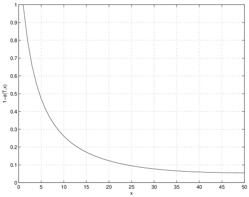
Figure 1. Bankrupt probability $1-\phi(T,x)$ as a function of $x$ (Parameters: $\sigma^{2}=\mu=1,\sigma^{2}_{p}=2,T=1,m=1,b=50$)

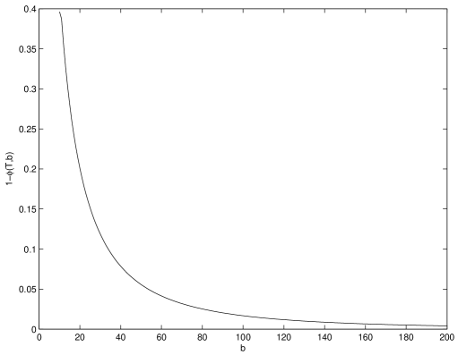
Figure 2. Bankrupt probability $1-\phi(T,b)$ as a function of $b$( Parameters: $\sigma^{2}=\mu=1,\sigma^{2}_{p}=2,T=1,m=1$)

Example 5.2.

Let $\sigma^{2}=\mu=1,\sigma^{2}_{p}=2,T=1,m=1$ and solve $b(\varepsilon)$ by $1-\phi(T,b)=\varepsilon$, we get the figure 3. It shows that the risk $\varepsilon$ greatly impacts on dividend payout level $b$. The dividend payout level $b$ decreases with the risk $\varepsilon$, so the risk $\varepsilon$ increases the company’s profit.

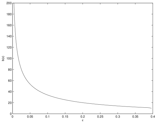
Figure 3. Dividend payout level $b(\varepsilon)$ as a function of $\varepsilon$ (Parameters: $\sigma^{2}=\mu=1,\sigma^{2}_{p}=2,T=1,m=1$ )

Example 5.3.

Let $\sigma^{2}=\mu=1,\sigma^{2}_{p}=2,T=1$ and solve $b(\varepsilon)$ by $1-\phi(T,b)=\varepsilon$, we get the figure 4 below. The two curves in this figure show that the minimum reserve requirement $m$ increases dividend payout level $b$, but decreases the company’s profit.

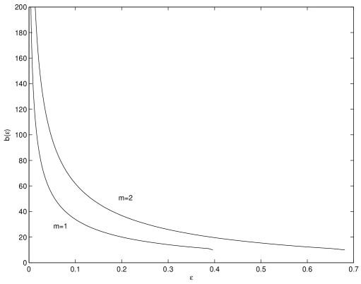
Figure 4. Dividend payout level $b(\varepsilon)$ as a function of $\varepsilon$ (Parameters: $\sigma^{2}=\mu=1,\sigma^{2}_{p}=2,T=1$).

Example 5.4.

Let $\sigma^{2}=\mu=1,\sigma^{2}_{p}=2,m=1$ and solve $b(\varepsilon)$ by $1-\phi(T,b)=\varepsilon$, we get the figure 5 below. It portrays that the dividend payout level $b$ is an increasing function of time horizon $T$, so it decreases the company’s profit.

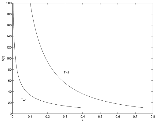
Figure 5. Dividend payout level $b(\varepsilon)$ as a function of $\varepsilon$ ( Parameters:$\sigma^{2}=\mu=1,\sigma^{2}_{p}=2,m=1$).

Example 5.5.

Let $\mu=1,\sigma^{2}_{p}=2,m=1$ and solve $b(\varepsilon)$ by $1-\phi(T,b)=\varepsilon$, we get the figure 6 below. It portrays that the dividend payout level $b$ is an increasing function of underwriting risk $\sigma^{2}$, so it decreases the company’s profit.

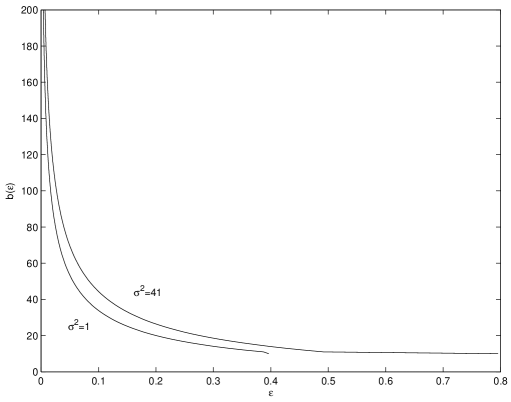
Figure 6. Dividend payout level $b(\varepsilon)$ as a function of $\varepsilon$ ( Parameters: $\mu=1,\sigma^{2}_{p}=2,m=1$).

6. Properties on bankrupt probability and $V(x,b)$

In this section, to prove Theorem 3.1, we list some lemmas on properties of bankrupt probability and $V(x,b)$ which will be used late. The rigorous proofs of these lemmas will be given in the appendix below.

Lemma 6.1.

The probability of bankruptcy $\mathbb{P}[\tau_{b}^{b}\leq T]$ is a decreasing function of $b$, where $\tau_{b}^{b}:=\tau_{b}^{\pi^{*}_{b}}$.

Lemma 6.2.

$$\lim_{b\rightarrow\infty}\mathbb{P}[\tau_{b}^{b}\leq T]=0.$$ (6.1)

Lemma 6.3.

Let $\phi(t,x)\in C^{1}(0,\infty)\cap C^{2}(m,b)$ and satisfy the following partial differential equation

$$\left\{\begin{array}[]{l l l}\phi_{t}(t,y)=\frac{1}{2}[{a^{\ast}}^{2}(x)\sigma^{2}+\sigma_{p}^{2}x^{2}]\phi_{xx}(t,x)+[a^{\ast}(x)\mu+rx]\phi_{x}(t,x),\\ \phi(0,x)=1,\ \mbox{for}\ \ m<x\leq b,\\ \phi(t,m)=0,\phi_{x}(t,b)=0,\ \mbox{for}\ t>0.\end{array}\right.$$ (6.5)

Then $\phi(T,x)=1-\psi^{b}(T,x)$, i.e., $\phi^{b}(T,x)$ is probability that the company will survive on time interval $[0,T]$, the function $\psi^{b}(t,x)$ is defined by

$$\psi^{b}(t,x):=\mathbb{P}[\tau_{x}^{b}\leq t],$$

where $\tau_{b}^{x}:=\tau_{x}^{\pi^{*}_{b}}$, i.e., probability of bankruptcy for the process $\{R_{t}^{\pi^{*}_{b},x}\}_{t\geq 0}$ with the initial asset $x$ and a dividend barrier $b$ is employed before time $t$. where $a^{\ast}(\cdot)$ is defined by (3.8).

Let $\sigma(x):=\frac{1}{2}[{a^{\ast}}^{2}(x)\sigma^{2}+\sigma_{p}^{2}x^{2}]$ and $\mu(x):=a^{\ast}(x)\mu+rx$. Then the equation (6.5) becomes

$$\phi_{t}(t,x)=\sigma^{2}(x)\phi_{xx}(t,x)+\mu(x)\phi_{x}(t,x).$$ (6.6)

By properties of $a^{\ast}(\cdot)$, it is easy to show that $\sigma(x)$ and $\mu(x)$ are continuous in $[m,b]$. So there exists a unique solution (6.5) and the solution is in $C^{1}(0,\infty)\cap C^{2}(m,b)$. Moreover, $\sigma^{{}^{\prime}}(x)$ and $\mu^{{}^{\prime}}(x)$ are bounded on $(m,x_{0})$ and $(x_{0},b)$ respectively.

Lemma 6.4.

Let $\phi^{b}(t,x)$ be a solution of the equation(6.5). Then the $\phi^{b}(T,b)$ is a continuous function of $b$ on $[b_{0},\infty)$.

Lemma 6.5.

Let $F_{b}(x)$ be defined by (3.5) and $b_{0}$ be given by part (ii) of Lemma 3.1. Then

$$\mathcal{L}F_{b}(x)\leq 0,\ \mbox{ for all $x\geq 0$},$$ (6.7)

where

$$\mathcal{L}=\frac{1}{2}(a^{2}\sigma^{2}+\sigma_{p}^{2}x^{2})\frac{d^{2}}{dx^{2}}+(a\mu+rx)\frac{d}{dx}-c.$$

Lemma 6.6.

(i) For any $b\leq b_{0}$ we have $V(x,b)=V(x,b_{0})=V(x)=F_{b_{0}}(x)=J(x,\pi_{b_{o}}^{\ast})$. Moreover, the optimal policy is $\pi_{b_{o}}^{\ast}=\{a^{\ast}(R^{\pi_{b_{o}}^{\ast}}_{t}),L^{\pi_{b_{o}}^{\ast}}_{t}\}$, where $(R^{\pi_{b_{o}}^{\ast}}_{t},L^{\pi_{b_{o}}^{\ast}}_{t})$ is uniquely determined by the SDE (3.13).
(ii) For any $b\geq b_{0}$ we have $V(x,b)=F_{b}(x)=J(x,\pi_{b}^{\ast})$. The optimal policy $\pi_{b}^{\ast}=\{a^{\ast}(R^{\pi_{b}^{\ast}}_{t}),L^{\pi_{b}^{\ast}}_{t}\}$, where $(R^{\pi_{b}^{\ast}}_{t},L^{\pi_{b}^{\ast}}_{t})$ is uniquely determined by the SDE(3.21).

The lemma 6.6 mainly deals with relationships among $F_{b}(x)$, $V(x,b)$ and $V(x)$ defined by (2).

Lemma 6.7.

For any $b\geq b_{0}$ and $x\geq m$,

$$\frac{d}{db}V(x,b)<0.$$ (6.8)

Moreover, if $b_{1},b_{2}\geq b_{0}$ and $x\leq\min\{b_{1},b_{2}\}$, then

$$\frac{V(x,b_{1})}{V(x,b_{2})}=\frac{h^{\prime}(b_{2})}{h^{\prime}(b_{1})}.$$ (6.9)

7. Appendix

In this section we will give the proofs of theorem and lemmas we concerned with throughout this paper. Proof of theorem 3.1.  If $\mathbb{P}[\tau_{b_{0}}^{b_{0}}\leq T]\leq\varepsilon$, then the conclusion is obvious because it is just the optimal control problem without constraints. Assume that $\mathbb{P}[\tau_{b_{0}}^{b_{0}}\leq T]>\varepsilon$. By Lemma 6.1 and Lemma 6.2, there exists a unique $b^{\ast}(\geq b_{0})$ such that

$$b^{\ast}=\min\{b:\mathbb{P}[\tau_{b}^{b}\leq T]=\varepsilon\}=\min\{b:b\in\mathfrak{B}\},$$ (7.1)

$$\mathbb{P}[\tau_{b}^{b}\leq T]>\varepsilon,\quad\forall b\leq b^{\ast},$$

$$\mathbb{P}[\tau_{b}^{b}\leq T]\leq\varepsilon,\quad\forall b\geq b^{\ast}.$$

By Lemma 6.7, we know that $V(x,b)$ is decreasing w.r.t. $b$, so $b^{\ast}$ satisfies(3.14). Using Lemma 6.4, we get $b^{\ast}\in\mathfrak{B}$ and $\mathbb{P}[\tau_{b^{\ast}}^{b^{\ast}}\leq T]=\varepsilon$. Moreover, by Lemma 6.6 and (7.1), we have

$$F_{b^{\ast}}(x)=V(x,b^{\ast})=J(x,\pi_{b^{*}}^{\ast})=V(x).$$

So the optimal policy associated with the optimal return function$V(x)$ is $\{a^{\ast}(R^{\pi_{b^{*}}^{\ast}}_{t}),L^{\pi_{b^{*}}^{\ast}}_{t}\}$, where, $(R^{\pi_{b^{*}}^{\ast}}_{t},L^{\pi_{b^{*}}^{\ast}}_{t})$ is determined uniquely by (3.21). The inequality (3.22) is a direct consequence of (6.9). $\Box$ Proof of lemma 6.1.   The proof of this lemma is the same as that of Theorem 3.1 in the [20], we omit it here. $\Box$ Proof of lemma 6.2.  Using the same argument as in the proof of theorem 3.1 in the [20], we have for some $n>3$ and large $b\geq\max\{1,m^{n}\}$

$$\mathbb{P}[\tau^{b}_{\sqrt[n]{b}}\leq T]\geq\mathbb{P}[\tau_{b}^{b}\leq T].$$ (7.2)

Let $R_{t}^{(2)}$ be the unique solution of the following SDE

$$dR_{t}^{(2)}=(a^{\ast}(R_{t}^{(2)})\mu+rR_{t}^{(2)})dt+\sqrt{{a^{\ast}}^{2}(R_{t}^{(2)})\sigma^{2}+\sigma_{p}^{2}{R_{t}^{(2)}}^{2}}dW_{t},$$

$$R_{0}^{(2)}=\sqrt[n]{b}.$$ (7.3)

Then by comparison theorem on SDE ( see Ikeda and Watanabe [17](1981))

$$\{\tau_{\sqrt[n]{b}}^{\pi^{*}_{b}}\leq T\}\subseteq\{\exists\ t\leq T\ \mbox{such that}\ R_{t}^{(2)}=m\ \mbox{ or}\ R_{t}^{(2)}=b\}.$$

As a result,

$$\mathbb{P}\{\tau_{\sqrt[n]{b}}^{\pi^{*}_{b}}\leq T\} \leq \mathbb{P}\{\exists\ t\leq T\ \mbox{such that}\ R_{t}^{(2)}=m\ \mbox{ or}\ R_{t}^{(2)}=b\}$$ (7.4)

$$\leq \mathbb{P}\{\sup_{0\leq t\leq T}R_{t}^{(2)}\geq b\}+\mathbb{P}\{\inf_{0\leq t\leq T}R_{t}^{(2)}\leq m\}.$$

Firstly, we estimate $\mathbb{P}\{\sup_{0\leq t\leq T}R_{t}^{(2)}\geq b\}$.Using Hölder inequality and $a^{*}(x)\leq 1$, it follows from SDE (7) that

$$\sup_{0\leq t\leq T}(R_{t}^{(2)})^{2} \leq [3(\sqrt[n]{b})^{2}+6\mu^{2}T^{2}]+6r^{2}T\int^{T}_{0}\sup_{0\leq s\leq t}(R_{s}^{(2)})^{2}ds$$ (7.5)

$$+ 3\sup_{0\leq t\leq T}\big{(}\int^{t}_{0}\sqrt{{a^{\ast}}^{2}(R_{s}^{(2)}\big{)}\sigma^{2}+\sigma_{p}^{2}{R_{s}^{(2)}}^{2}}dW_{s})^{2}.$$

Taking mathematical expectation at both sides of (7.5) and using B-D-G inequality, we derive

$$\mathbb{E}\{\sup_{0\leq t\leq T}(R_{t}^{(2)})^{2}\} \leq [3(\sqrt[n]{b})^{2}+6\mu^{2}T^{2}]+6r^{2}T\int^{T}_{0}\mathbb{E}\{\sup_{0\leq s\leq t}(R_{s}^{(2)})^{2}\}ds$$ (7.6)

$$+12\mathbb{E}\{\int^{T}_{0}({a^{\ast}}^{2}(R_{s}^{(2)})\sigma^{2}+\sigma_{p}^{2}{R_{s}^{(2)}}^{2})dt\}$$

$$\leq \big{[}3(\sqrt[n]{b})^{2}+6\mu^{2}T^{2}+12\sigma^{2}T^{2}\big{]}$$

$$+6(r^{2}T+2\sigma^{2}_{p})\int^{T}_{0}\mathbb{E}\{\sup_{0\leq s\leq t}(R_{s}^{(2)})^{2}\}ds.$$

Solving (7.6), we get

$$\mathbb{E}\{\sup_{0\leq t\leq T}(R_{t}^{(2)})^{2}\} \leq \big{[}(3\sqrt[n]{b})^{2}+6\mu^{2}T^{2}+12\sigma^{2}T^{2}\big{]}\exp\{6(r^{2}T+2\sigma^{2}_{p})T\}.$$

Combining Markov inequality and the inequality (7), we conclude that

$$\mathbb{P}\{\sup_{0\leq t\leq T}R_{t}^{(2)}\geq b\} \leq \frac{\mathbb{E}\{\sup_{0\leq t\leq T}(R_{t}^{(2)})^{2}\}}{b^{2}}$$

$$\leq \frac{\big{(}3(\sqrt[n]{b})^{2}+6\mu^{2}T^{2}+12\sigma^{2}T^{2}\big{)}\exp\{6(r^{2}T+2\sigma^{2}_{p})T\}}{b^{2}}.$$

Secondly, we estimate $\mathbb{P}\{\inf_{0\leq t\leq T}R_{t}^{(2)}\leq m\}$. Let $M_{1}$ be a martingale defined by

$$M_{1}(t)=\int^{t}_{0}I_{\{s:R_{s}^{(2)}\neq 0\}}\sqrt{\sigma^{2}(\frac{a^{\ast}(R_{s}^{(2)})}{R_{s}^{(2)}})^{2}+\sigma_{p}^{2}}\quad dW_{s}.$$

Then we can rewrite the SDE (7) as follows,

$$R_{t}^{(2)}=\big{(}\sqrt[n]{b}+\int^{t}_{0}(a^{\ast}(R_{s}^{(2)})\mu+rR_{s}^{(2)})ds\big{)}+\int^{t}_{s}R_{s}^{(2)}dM_{1}(s).$$

In view of Proposition 2.3 of Chapter 9 in [25],

$$R_{t}^{(2)}=\mathcal{E}(M_{1})_{t}\big{(}\sqrt[n]{b}+\int^{t}_{0}\frac{(\mu a^{\ast}(R_{s}^{(2)})+rR_{s}^{(2)})}{\mathcal{E}(M_{1})_{s}}ds\big{)},$$

where $\mathcal{E}(M_{1})_{t}=\exp\{M_{1}(t)-\frac{1}{2}<M_{1}>(t)\}$ is an exponential martingale, $<M_{1}>$ is the bracket of $M_{1}$. So the fact $\inf{\{f(t)g(t)\}}\geq\inf\{f(t)\}\inf\{g(t)\}$ for any $f(t)\geq 0$ and $g(t)\geq 0$ implies that

$$\inf_{0\leq t\leq T}\{R_{t}^{(2)}\}\geq\sqrt[n]{b}\inf_{0\leq t\leq T}\{\mathcal{E}(M_{1})_{t}\}.$$

As a result

$$\mathbb{P}\{\inf_{0\leq t\leq T}R_{t}^{(2)}\leq m\}\leq\mathbb{P}\{\inf_{0\leq t\leq T}\mathcal{E}(M_{1})_{t}\leq\frac{m}{\sqrt[n]{b}}\}.$$

Since $<M_{1}>_{T}\leq(\lambda^{2}\sigma^{2}+\sigma_{p}^{2})T<+\infty$, we have

$$\lim_{b\longrightarrow\infty}\mathbb{P}\{\inf_{0\leq t\leq T}R_{t}^{(2)}\leq m\} \leq \mathbb{P}\{\inf_{0\leq t\leq T}\mathcal{E}(M_{1})_{t}=0\}$$ (7.9)

$$\leq \mathbb{P}\{\sup_{0\leq t\leq T}|M_{1}(t)|=+\infty\}.$$

By B-D-G inequalities, we get

$$\mathbb{E}\{\sup_{0\leq t\leq T}|M_{1}(t)|^{2}\}\leq 4(\lambda^{2}\sigma^{2}+\sigma_{p}^{2})T<+\infty,$$

which implies that

$$\mathbb{P}\{\sup_{0\leq t\leq T}|M_{1}(t)|=+\infty\}=0.$$

Thus by (7.9)

$$\lim_{b\longrightarrow\infty}\mathbb{P}\{\inf_{0\leq t\leq T}\{R_{t}^{(2)}\}\leq m\}=0.$$ (7.10)

So the inequalities (7.2), (7.4), (7) and (7.10) yield that

$$\lim_{b\rightarrow\infty}\mathbb{P}\{\tau_{{b}}^{\pi^{*}_{b}}\leq T\}=0.$$

$\Box$

Remark 7.1.

The proof of theorem 3.2 in [20] seems wrong, so we can use the way proving Lemma 6.2 to correct it. Theorem 3.2 in the [20] is indeed a direct consequence of Lemma 6.2.

Proof of lemma 6.3. Let $(R_{t}^{b},L_{b}(t))$ denote $(R^{\pi_{b}^{\ast}}_{t},L^{\pi_{b}^{\ast}}_{t})$ defined by SDE (4.6). Since $(R_{t}^{b},L_{b}(t))$ is continuous process, by the generalized Itô formula, we have

$$\phi(T-(t\wedge\tau_{x}^{b}),R_{t\wedge\tau_{x}^{b}}^{b}) = \phi(T,x)$$ (7.11)

$$+ \int_{0}^{t\wedge\tau_{x}^{b}}\{\frac{1}{2}[{a^{\ast}}^{2}(R_{s}^{b})\sigma^{2}+\sigma_{p}^{2}\cdot(R_{s}^{b})^{2}]\sigma^{2}\phi_{xx}(T-s,R_{s}^{b})$$

$$+ [a^{*}(R_{s}^{b})\mu+rR_{s}^{b}]\phi_{x}(T-s,R_{s}^{b})$$

$$- \phi_{t}(T-s,R_{s}^{b})\}ds-\int_{0}^{t\wedge\tau_{x}^{b}}\phi_{x}(T-s,R_{s}^{b})dL_{b}(s)$$

$$+ \int_{0}^{t\wedge\tau_{x}^{b}}a(R_{s}^{b})\sigma\phi_{x}(T-s,R_{s}^{b})dW_{s}.$$

Letting $t=T$ and taking mathematical expectation at both sides of (7.11) yields that

$$\phi(T,x) = \mathbb{E}[\phi(T-(T\wedge\tau_{x}^{b}),R_{T\wedge\tau_{x}^{b}}^{b})]$$

$$= \mathbb{E}[\phi(0,R_{T}^{b})1_{T<\tau_{x}^{b}}]+\mathbb{E}[\phi(T-\tau_{x}^{b},m)1_{T\geq\tau_{x}^{b}})]$$

$$= \mathbb{E}[1_{T<\tau_{x}^{b}}]=\mathbb{P}[\tau_{x}^{b}>T]=1-\psi(T,x).$$

$\Box$ Now we use PDE method to prove lemma 6.4. Proof of lemma 6.4.   Let $x=by,0\leq y\leq 1$ and $\theta^{b}(t,y)=\phi^{b}(t,(b-m)y+m)$. Then the equation (6.5) becomes

$$\left\{\begin{array}[]{l l l}\theta_{t}^{b}(t,y)=[\sigma[(b-m)y+m]/(b-m)^{2}]\theta_{yy}^{b}(t,y)\\ +[\mu[(b-m)y+m]/(b-m)]\theta_{y}^{b}(t,y),\\ \theta^{b}(0,y)=1,\ \mbox{for}\ 0\leq y\leq 1,\\ \theta^{b}(t,0)=0,\theta_{y}^{b}(t,1)=0,\ \mbox{for}\ t>0.\end{array}\right.$$ (7.16)

In view of (7.16), the proof of Lemma 6.4 reduces to proving $\lim\limits_{b_{2}\rightarrow b_{1}}\theta^{b_{2}}(t,1)=\theta^{b_{1}}(t,1)$ for fixed $b_{1}>b_{0}$. Let $w(t,y)=\theta^{b_{2}}(t,y)-\theta^{b_{1}}(t,y)$. Since $\theta^{b}(t,y)$ is continuous at $y=1$ for any $b>b_{0}$, we only need to show that

$$\int_{0}^{t}\int_{0}^{1}w^{2}(s,y)dsdy\rightarrow 0,\mbox{as $b_{2}\rightarrow b_{1}$}.$$ (7.17)

Let $\sigma^{b}(y)=\sigma[(b-m)y+m]/(b-m)^{2}$, $\mu^{b}(y)=\mu[(b-m)y+m]/(b-m)$. Then the (7.16) translates into

$$\left\{\begin{array}[]{l l l}w_{t}(t,y)&=&\sigma^{b_{2}}(y)w_{yy}(t,y)+\mu^{b_{2}}(y)w_{y}(t,y)\\ &+&\{\sigma^{b_{2}}(y)-\sigma^{b_{1}}(y)\}\theta_{yy}^{b_{1}}(t,y)\\ &+&\{\sigma^{b_{2}}(y)-\sigma^{b_{1}}(y)\}\theta_{y}^{b_{1}}(t,y),\\ w(0,y)&=&0,\ \mbox{for}\ 0<y\leq 1,\\ w(t,y)&=&0,y=0,\ w_{y}(t,1)=0,\ \mbox{for}\ t>0.\end{array}\right.$$ (7.23)

Multiplying both sides of the first equation in (7.23) by $w(t,z)$, and then integrating both sides of the resulting equation on $[0,t]\times[0,1]$, we get

$$\int_{0}^{t}\int_{0}^{1}w(s,y)w_{t}(s,y)dyds$$ (7.24)

$$= \int_{0}^{t}\int_{0}^{1}[\sigma^{b_{2}}(y)]w(s,y)w_{yy}(s,y)dyds$$

$$+ \int_{0}^{t}\int_{0}^{1}[\mu^{b_{2}}(y)]w(s,y)w_{y}(s,y)dyds$$

$$+ \int_{0}^{t}\int_{0}^{1}[\sigma^{b_{2}}(y)-\sigma^{b_{1}}(y)]w(s,y)\theta_{yy}^{b_{1}}(t,y)dyds$$

$$+ \int_{0}^{t}\int_{0}^{1}w(s,y)[\mu^{b_{2}}(y)-\mu^{b_{1}}(y)]w(s,y)\theta_{y}^{b_{1}}(t,y)dyds$$

$$\equiv E_{1}+E_{2}+E_{3}+E_{4}.$$

Now we look at terms at both sides of (7.24). Firstly, we have

$$\int_{0}^{t}\int_{0}^{1}w(s,y)w_{t}(s,y)dyds = \int_{0}^{1}\frac{1}{2}w^{2}(t,y)dy.$$ (7.25)

Secondly, we deal with terms $E_{i}$, $i=1,\cdots,4$ as follows. It is easy to see from the expression of $a^{\ast}(\cdot)$ that there exist positive constants $D_{1}$, $D_{2}$ and $D_{3}$ such that $[\mu(b_{2}y)/b_{2}]^{2}\leq D_{1}$ and $\sigma^{b}_{2}(y)\geq D_{2}>0$ for $y\geq 0$, and $\sigma^{b}_{2}(y)^{\prime}\leq D_{3}$ for $y\in(0,\frac{x_{0}-m}{b-m})\cup(\frac{x_{0}-m}{b-m},1]$. As a result, for any $\lambda_{1}>0$ and $\lambda_{2}>0$

$$E_{1} = \int_{0}^{t}\int_{0}^{1}[\sigma^{b_{2}}(y)]w(s,y)w_{yy}(s,y)dyds$$ (7.26)

$$= -\int_{0}^{t}\int_{0}^{1}[\sigma^{b_{2}}(y)]w_{y}^{2}(s,y)dyds$$

$$-\int_{0}^{t}[\int_{0}^{(x_{0}-m)/(b-m)}+\int_{(x_{0}-m)/(b-m)}^{1}][\sigma^{b_{2}}(y)]^{{}^{\prime}}w_{y}(s,y)w(s,y)dyds$$

$$\leq -D_{2}\int_{0}^{t}\int_{0}^{1}w_{y}^{2}(s,y)dyds$$

$$+D_{3}\int_{0}^{t}\int_{0}^{1}\lambda_{1}w_{y}^{2}(s,y)+\frac{1}{4\lambda_{1}}w^{2}(s,y)dyds$$

and

$$E_{2} = \int_{0}^{t}\int_{0}^{1}[\mu^{b_{2}}(y)]w(s,y)w_{y}(s,y)$$ (7.27)

$$\leq \lambda_{2}\int_{0}^{t}\int_{0}^{1}w_{y}^{2}(s,y)dyds$$

$$+\frac{D_{1}}{4\lambda_{2}}\int_{0}^{t}\int_{0}^{1}w^{2}(s,y)dyds.$$

In order to estimate $E_{3}$, we decompose $E_{3}$ as follows:

$$E_{3} = \int_{0}^{t}\int_{0}^{1}\{\sigma^{b_{2}}(y)-\sigma^{b_{1}}(y)\}w(s,y)\theta_{yy}^{b_{1}}(s,y)dyds$$ (7.28)

$$= -\int_{0}^{t}\int_{0}^{1}\{\sigma^{b_{2}}(y)-\sigma^{b_{1}}(y)\}w_{y}(s,y)\theta_{y}^{b_{1}}(s,y)dyds$$

$$-\int_{0}^{t}\int_{0}^{(x_{0}-m)/(b_{2}-m)}\{\sigma^{b_{2}}(y)-\sigma^{b_{1}}(y)\}^{\prime}w(s,y)\theta_{y}^{b_{1}}(s,y)dyds$$

$$-\int_{0}^{t}\int_{(x_{0}-m)/(b_{2}-m)}^{(x_{0}-m)/(b_{1}-m)}\{\sigma^{b_{2}}(y)-\sigma^{b_{1}}(y)\}^{\prime}w(s,y)\theta_{y}^{b_{1}}(s,y)dyds$$

$$-\int_{0}^{t}\int_{(x_{0}-m)/(b_{1}-m)}^{1}\{\sigma^{b_{2}}(y)-\sigma^{b_{1}}(y)\}^{\prime}w(s,y)\theta_{y}^{b_{1}}(s,y)dyds$$

$$= E_{31}+E_{32}+E_{33}+E_{34}.$$

So the estimating $E_{3}$ is reduced to estimating $E_{3i}$, $i=1,\cdots,4$. The fact $[\sigma(by)/b^{2}]$, $[\sigma(by)/b^{2}]^{\prime}$and $[\mu(by)/b]$ are Lipschitz continuous on $(0,\frac{x_{0}-m}{b_{2}-m})$, $(\frac{x_{0}-m}{b_{2}-m},\frac{x_{0}-m}{b_{1}-m})$ and $(\frac{x_{0}-m}{b_{1}-m},1)$, that is, there exists $L>0$ such that

$$|[\sigma^{b_{2}}(y)]-[\sigma^{b_{1}}(y)]|\leq L|b_{2}-b_{1}|,$$

$$|[\sigma^{b_{2}}(y)]^{\prime}-[\sigma^{b_{1}}(y)]^{\prime}|\leq L|b_{2}-b_{1}|,$$

$$|[\mu^{b_{2}}(y)]-[\mu^{b_{1}}(y)]|\leq L|b_{2}-b_{1}|,$$

and Young’s inequality yield that for any $\lambda_{3}>0$ and $\lambda_{4}>0$

$$E_{31} = -\int_{0}^{t}\int_{0}^{1}[\sigma^{b}_{2}(y)-\sigma^{b}_{1}(y)]w_{y}(s,y)\theta_{y}^{b_{1}}(s,y)dyds$$ (7.29)

$$\leq \frac{L^{2}(b_{2}-b_{1})^{2}}{4\lambda_{3}}\int_{0}^{t}\int_{0}^{1}[\theta_{y}^{b_{1}}(s,y)]^{2}dyds$$

$$+\lambda_{3}\int_{0}^{t}\int_{0}^{1}w_{y}^{2}(s,y)dyds,$$

$$E_{32}+E_{34} = -\int_{0}^{t}\big{[}\int_{0}^{(x_{0}-m)/(b_{2}-m)}+\int_{(x_{0}-m)/(b_{1}-m)}^{1}\big{]}\{\sigma^{b_{2}}(y)$$ (7.30)

$$- \sigma^{b_{1}}(y)\}^{\prime}w(s,y)\theta_{y}^{b_{1}}(s,y)dyds$$

$$\leq \frac{L^{2}(b_{2}-b_{1})^{2}}{4\lambda_{4}}\int_{0}^{t}\int_{0}^{1}[\theta_{y}^{b_{1}}(s,y)]^{2}dyds$$

$$+\lambda_{4}\int_{0}^{t}\int_{0}^{1}w^{2}(s,y)dyds.$$

The remaining part of estimating $E_{3}$ is to deal with $E_{33}$.By the boundary conditions

$$0 = \int_{0}^{t}\int_{0}^{1}\theta_{t}^{b}(s,y)\theta^{b}(s,y)$$

$$-\sigma^{b}(y)\theta_{yy}^{b}(s,y)\theta^{b}(s,y)-\mu^{b}(y)\theta_{y}^{b}(s,y)\theta^{b}(s,y)dyds$$

$$= \frac{1}{2}\int_{0}^{1}[\theta^{b}(s,y)]^{2}dy+\int_{0}^{t}\int_{0}^{1}\sigma^{b}(y)[\theta_{y}^{b}(s,y)]^{2}dyds$$

$$+\int_{0}^{t}\big{[}\int_{0}^{(x_{0}-m)/(b-m)}+\int_{(x_{0}-m)/(b-m)}^{1}\big{]}\sigma^{b}(y)^{\prime}[\theta_{y}^{b}(s,y)][\theta^{b}(s,y)]dyds$$

$$= \frac{1}{2}\int_{0}^{1}[\theta^{b}(s,y)]^{2}dy+\int_{0}^{t}\int_{0}^{1}\sigma^{b}(y)[\theta_{y}^{b}(s,y)]^{2}dyds$$

$$+\int_{0}^{t}\big{[}\int_{0}^{(x_{0}-m)/(b-m)}+\int_{(x_{0}-m)/(b-m)}^{1}\big{]}(\sigma^{b}(y)^{\prime}$$

$$-\mu^{b}(y))[\theta_{y}^{b}(s,y)][\theta^{b}(s,y)]dyds$$

$$\geq \lambda_{5}\int_{0}^{t}\int_{0}^{1}[\theta_{y}^{b}(s,y)]^{2}dyds-\frac{\lambda_{5}}{2}\int_{0}^{t}\int_{0}^{1}[\theta_{y}^{b}(s,y)]^{2}dyds$$

$$-\frac{\lambda_{6}}{2\lambda_{5}}\int_{0}^{t}\int_{0}^{1}[\theta^{b}(s,y)]^{2}dyds$$

$$\geq \frac{\lambda_{5}}{2}\int_{0}^{t}\int_{0}^{1}[\theta_{y}^{b}(s,y)]^{2}dyds-\frac{\lambda_{6}}{2\lambda_{5}},$$

from which we know that

$$\int_{0}^{t}\int_{0}^{1}[\theta_{y}^{b}(s,y)]^{2}dyds\leq\frac{\lambda_{6}}{\lambda_{5}^{2}},$$

where $\lambda_{5}>0$ is the lower boundary of $\sigma^{b}(y)$ and $\lambda_{6}$ is the upper boundary of $|[\sigma(by)/b^{2}]^{\prime}-[\mu(by)/b]|$ on $(0,\frac{x_{0}-m}{b-m})\cup(\frac{x_{0}-m}{b-m},1]$.Therefore we conclude that $\int_{0}^{t}\int_{0}^{1}[\theta_{y}^{b}(s,y)]^{2}dyds$ is bounded. So by using $w(s,y)\leq 2$, we have

$$\lim_{b_{2}\rightarrow b_{1}}|E_{33}|=0.$$ (7.31)

Thus the equalities (7.29),(7.30) and (7.31) yield that there exists a positive function $B_{1}^{b_{1}}(b_{2})$ with $\lim\limits_{b_{2}\rightarrow b_{1}}B_{1}^{b_{1}}(b_{2})=0$ such that for $0\leq t\leq T$

$$E_{3} = \int_{0}^{t}\int_{0}^{1}\{\sigma(b_{2}y)/b_{2}^{2}-\sigma(b_{1}y)/b_{1}^{2}\}w(s,y)\theta_{yy}^{b_{1}}(t,y)dyds$$

$$= E_{31}+E_{32}+E_{33}+E_{34}$$

$$\leq B^{b_{1}}(b_{2})+(\lambda_{3}+\lambda_{4})\int_{0}^{t}\int_{0}^{1}w_{y}^{2}(s,y)+w^{2}(s,y)dyds.$$

By the same way as that of (7.27)

$$E_{4} = \int_{0}^{t}\int_{0}^{1}\{\mu(b_{2}y)/b_{2}-\mu(b_{1}y)/b_{1}\}w(s,y)\theta_{y}^{b_{1}}(t,y)dyds$$ (7.33)

$$\leq \frac{L^{2}(b_{2}-b_{1})^{2}}{4\lambda_{7}}\int_{0}^{t}\int_{0}^{1}[\theta_{y}^{b_{1}}(s,y)]^{2}dyds$$

$$+\lambda_{7}\int_{0}^{t}\int_{0}^{1}w^{2}(s,y)dyds.$$

Let

$$B_{2}^{b_{1}}(b_{2})=\frac{L^{2}(b_{2}-b_{1})^{2}}{4\lambda_{7}}\int_{0}^{t}\int_{0}^{1}[\theta_{y}^{b_{1}}(s,y)]^{2}dyds.$$

Then

$$\lim\limits_{b_{2}\rightarrow b_{1}}B_{2}^{b_{1}}(b_{2})=0,$$

which, together with (7.33), implies that

$$E_{4}\leq B_{2}^{b_{1}}(b_{2})+\lambda_{7}\int_{0}^{t}\int_{0}^{1}w^{2}(s,y)dyds.$$ (7.34)

Choosing $\lambda_{1}$, $\lambda_{2}$ and $\lambda_{3}$ small enough such that$\lambda_{1}+D_{3}\lambda_{2}+\lambda_{3}<D_{2}$, we can conclude from $(\ref{eq4.16})$, (7.26), (7.27), (7) and (7.34) that there exist constants $C_{1}$ and $C_{2}$ such that

$$\int_{0}^{1}w^{2}(t,y)dy\leq C_{1}\int_{0}^{t}\int_{0}^{1}w^{2}(s,y)dyds+C_{2}[B_{1}^{b_{1}}(b_{2})+B_{2}^{b_{1}}(b_{2})].$$

Using the Gronwall inequality, we get

$$\int_{0}^{t}\int_{0}^{1}w^{2}(s,y)dyds\leq C_{2}[B_{1}^{b_{1}}(b_{2})+B^{b_{1}}(b_{2})]\exp\{C_{1}t\}.$$

So

$$\lim\limits_{b_{2}\rightarrow b_{1}}\int_{0}^{t}\int_{0}^{1}[\theta^{b_{2}}(s,y)-\theta^{b_{1}}(s,y)]^{2}dyds=0.$$

Thus we complete the proof.  $\Box$ Proof of lemma 6.5.  If $x<m$ then by (3.5), $F_{b}(x)=0$. It suffices to prove (6.7) for $m\leq x$. If $m\leq x\leq b$, then

$$\mathcal{L}F_{b}(x)=\frac{\mathcal{L}h(x)}{h^{\prime}(b)},$$

here $h(x)$ is a solution of (3.1), so $\mathcal{L}F_{b}(x)\leq 0$ follows from lemma 3.1. If $x>b$ then by using $F_{b}^{\prime\prime}(b)\geq 0$ for $b\geq b_{0}$

$$\mathcal{L}F_{b}(x) = \frac{1}{2}(a^{2}\sigma^{2}+\sigma_{p}^{2}x^{2})F_{b}^{\prime\prime}(x)+(a\mu+rx)F_{b}^{\prime}(x)-cF_{b}(x)$$

$$\leq (\mu+rx)-c(x-b+F_{b}(b))$$

$$\leq (\mu+rb)-cF_{b}(b)$$

$$= \mathcal{L}F_{b}(b)-\frac{1}{2}(a^{2}\sigma^{2}+\sigma_{p}^{2}x^{2})F_{b}^{\prime\prime}(b)$$

$$\leq 0$$

Thus the proof follows. $\Box$ Proof of lemma 6.6.   The proof basically follows the same arguments as in the proof of theorem 5.2 in He and Liang [18] and so we omit it. $\Box$ Proof of lemma 6.7. The lemma is a direct consequence of lemma 6.5 and lemma 6.6. $\Box$

Acknowledgements. This work is supported by Project 10771114 of NSFC, Project 20060003001 of SRFDP, the SRF for ROCS, SEM and the Korea Foundation for Advanced Studies. We would like to thank the institutions for the generous financial support. We are very grateful to the referees for the careful reading of the manuscript, correction of errors, and valuable suggestions which improved the main results of this paper very much. Special thanks also go to the participants of the seminar stochastic analysis, finance and insurance at Tsinghua University for their feedbacks and useful conversations. Zongxia Liang is also very grateful to College of Social Sciences and College of Engineering at Seoul National University for providing excellent working conditions for him. The authors also thank Jicheng Yao for very valuable discussions on lemma 6.4.

References

- [1] Borch, K.,1969. The Capital Structure of a Firm, Swedish Journal of Econometrics 71, 1-13, 1969.
- [2] Borch, K. 1967. The Theory of Risk, Journal of the Royal statiscal Society , B 29, 432-452.
- [3] Choulli, T., Taksar, M. and Zhou, X.Y., 2001. Interplay between dividend rate and business constraints for a financial corporation. The Annals of Applied Probability 14(1), 1810-1837.
- [4] Bowers, Gerber, Hickman, Donald and Nesbitt, 1997. Actuarial mathematics. The society of actuaries, ISBN:0938959468.
- [5] Emanuel D C,Harrison, J.M. and Taylor A. J., 1975. A diffusion approximation for the ruin probability with compounding assets. Scandinavian Acturial Journal 75, 240-247.
- [6] Grandell J., 1977. A class of approximations of ruin probabilities. Scandinavian Acturial Journal Suppl.77, 37-52.
- [7] Grandell J., 1978. A remark on a class of approximations of ruin probabilities. Scandinavian Acturial Journal78, 77-78.
- [8] Grandell J. 1990. Aspect of risk theory ( New York: Springer).
- [9] Gerber, H. U.,1972. Games of Ecomonic Survival with Discrete and Continous Income Processes, Opns. Res. 20, 37-45.
- [10] Harrison, J.M., 1985. Brownian motion and stochastic flow systems( New York: Wiley).
- [11] Harrison, J.M.; Taksar, M.J.,1983. Instant control of Brownian motion, Mathematics of Operations Research. 8, 439-453.
- [12] Højgaard, B., Taksar, M.,1998. Optimal Proportional Reinsurance Policies for Diffusion Models. Scandinavian Acturial Journal 2, 166-180.
- [13] Højgaard, B., Taksar, M., 1999. Controlling Risk Exposure and Dividends Payout Schemes: Insurance company Example, Mathematical Finance 9(2), 153-182.
- [14] Højgaard, B., Taksar, M.,2001. Optimal Risk Control for a Large Corporation in the Presence of Returns on Investments, Finance and Stochast. 5, 527-547.
- [15] Iglehart D.L.,1969. Diffusion approximations in collective risk theory. J.App. Probab. 6. 285-292.
- [16] Ikeda, I. and Watanabe,1997. A comparison theorem for solutions of stochastic differential equations and its applications. Osaka J. Math. 14, 619-633.
- [17] Ikeda, N., Watanabe, S.,1981. Stochastic diffeential Equations and Diffusion Processes. North-Holland, ISBN 0444-86172-6.
- [18] Lin He, Zongxia Liang,2008. Optimal Financing and Dividend Control of the Insurance Company with Proportional Reinsurance Policy. Insurance: Mathematics and Economics 42, 976-983.
- [19] Lin He, Zongxia Liang,2009. Optimal Financing and Dividend Control of the Insurance Company with Fixed and Proportional Transaction Costs. Insurance: Mathematics and Economics 44, 88-94.
- [20] Lin He, Ping Hou and Zongxia Liang,2008. Optimal Control of the Insurance Company with proportional reinsurance policy under solvency constraints. Insurance: Mathematics and Economics 43, 474-479.
- [21] Lions, P.-L.; Sznitman, A.S.,1984. Stochastic differential equations with reflecting boundary conditions. Comm.Pure Appl. Math.37,511-537.
- [22] Paulsen, J., Gjessing, H. K.,1997. Optimal Choice of Dividend Barriers for a Risk Process with Stochastic Return of Investment, Insurance: Math. Econ. 20, 215-223.
- [23] Paulsen, J.,2003. Optimal dividend payouts for diffusions with solvency constraints. Finance and Stochastics 7, 457-473.
- [24] Radner, R., Sheep, L.,1996. Risk vs. Profit Potential: A Model for Corporate Strategy, J. Econ. Dynam. Control 20, 1373-1393.
- [25] Revuz D. and Yor, M.,1998. Continuous martingales and Brownian motion. Third edition, Springer.
- [26] Riegel and Miller,1963. Insurance Principle and practices. Prentice-Hall,Inc. Fourth edition.
- [27] Schmidli H., 1994. Diffusion approximations for a risk process with the possibility of borrowing and interest. Commun. Stat. Stochast. Models. 10, 365-388.
- [28] S.E.Shreve,J.P.Lehoczky and D.P.Gaver. 1984. Optimal Consumption for General Diffusions with Absorbing and Reflecting Barrier,SIAM ,Control and Optimization 22(1).
- [29] Welson and Taylor,1959. Insurance Administration. London Sir Isaac pitman and Sons, Ltd. Eighth edition.
- [30] C.A. Williams, Jr. and R.M. Heins,1985. Risk management and insurence. Mcgraw-Hill book company, fifth edition, ISBN:0070705615.