The equation of state of the n-vector model: collective variables method.

Abstract

The critical behavior of the three-dimensional n-vector model in the presence of an external field is investigated. Mathematical description is performed with the collective variables (CV) method in the framework of the $\rho^{4}$ model approximation at the microscopic level without any adjustable parameters. The recurrence relations of the renormalization group (RG) as functions of the external field and temperature were found. The analytical expression for the free energy of the system for temperatures $T>T_{c}$ and different n was obtained. The equation of state of the n-vector model for general case of small and large external fields was written. The explicit form of the correspondent scaling function for different values of the order parameter was derived. The obtained results are in qualitative agreement with the data of Monte Carlo simulations.

I Introduction

The investigation of the critical behavior of the real three-dimensional(3D) magnets is one of the most important problems of condensed matter physics. The present work is connected with investigation of the classical n-vector model on 3D simple cubic lattice in the presence of an external magnetic field by the collective variables (CV) method. Originally this method was introduced by Bom Bom , then used by Zubarev for systems of charged particles Zub and later developed for calculation of the thermodynamic and structural characteristics of 3D systems near the phase transition (PT) point 06 . The above mentioned model is well-known as the classical $O(n)$-vector model or, in field-theoretic language, as the $O(n)$-invariant nonlinear $\sigma$-model. Depending on components of an order parameter this model can describe a number of physical systems such as: polymers, ferromagnets, antiferromagnets, the critical point of the liquid-vapor transition, the Bose-condensation, phase transitions in binary alloys etc.

The investigations of the critical properties of the O(n)-vector models and their partial cases were carried out by various methods such as: high- and low-temperature expansions, the field theory, the semi-microscopic scaling field theory and Monte-Carlo simulations. In general, much attention was devoted to investigation of the universal characteristics of the system such as critical exponents and relations of the critical amplitudes of the thermodynamic functions.

The collective variables method as well as Wilson’s approach Wil is based on use of the hypothesis of scaling invariance and the renormalization group (RG) method for the phase transition theory suggested by Patashynskii, Pokrovskii Pok and Kadonoff Kad .

The RG method was used to obtain the equation of state of Ising system up to the order $\epsilon^{2}$ by Avdeiva and Migdal Avd and by Bresin, Wallace, Wilson Briz . The obtained results were generalized for the case of the n-vector model in Briz1 .

Besides, the positive results were achieved at calculation of the thermodynamic functions near the critical point. In Wegner’s work Weg was obtained expression for the free energy with taking into account the so-called ‘irrelevant’ operators in the Wilson’s approach. Riedel and Wegner Weg1 suggested the method of scaling fields for obtaining crossover scaling functions of the free energy and the susceptibility. The works of Fisher and Aharony Fish , Nicoll and Albright Nik and also Nelson Nel are dedicated to receiving of the crossover scaling functions for $T>T_{c}$ in zero magnetic field near four dimensions. In the frame of the massive field theory by Bagnuls and Bervillier Bag the explicit results for the correlation length, the susceptibility and the heat capacity as functions of the temperature in the disordered phase along the critical isochore for one-, two- and three-component systems were obtained. The non asymptotic behavior was described as crossover between the Wilson-Fisher’s (near the critical temperature $T_{c}$) and mean field’s (far from $T_{c}$) behaviors using three adjustable parameters. But this crossover can not realistically describe the situation in the system, because there are some physical restrictions of the model. Thus, in the works of Dohm and co-workers Domb1 ; Domb2 the calculation of the thermodynamical characteristics of the system without $\epsilon$-expansion was performed in the frame of some minimal subtraction scheme based on high-ordered perturbation theory and Borel resummation. This minimizing scheme is related to the use of the general relations between the heat capacity coefficients for approximation of the temperature dependence of coefficient $u(t)$ near the fourth term in the Ginsburg-Landau Hamiltonian. This method allows to obtain the non universal critical behavior of the thermodynamic functions below and above the critical temperature, such as the heat capacity and the susceptibility as functions of $u(t)$ without any adjustable parameters. But it does not provide possibility to analyze the dependence of the thermodynamic variables on the microscopic parameters of the interaction potential.

Besides, the essential success was achieved in calculation of the universal relations of the critical amplitudes. Okabe and Ohno Ok1 , Okabe and Ideura Ok2 investigated the relations of the critical amplitudes of the susceptibility by high-temperature-, 1/n- and $\epsilon$-expansion up to the order $O(\epsilon^{2})$. Bresin, Le Guillon and Zinn-Justin Brez calculated the universal relations of the critical amplitudes for the heat capacity, the susceptibility and the correlation length by Wilson-Fisher’s $\epsilon$-expansion.

It should be mentioned, that PT is actively investigated by Monte-Carlo (MC) method. Thus Ferrenberg and Landau Fer1 ; Fer2 found the critical temperature and critical exponents for the Ising and classical Heisenberg models using high-resolution MC method. Besides, the universal relations of the critical amplitudes and the equation of state were obtained by Engels for $O(1),\;O(2),\;O(4)$ models Eng1 ; Eng2 ; Eng4 and by Campostrini et al. for $O(3)$ model Camp .

A number of new results were obtained using for the description of PT the collective variables method. The specificity of the CV method is successive microscopic approach and the method of integration of the partition function by short-wave fluctuations without applying of the perturbation theory. In the frame of this method the general recurrence relations (RR) which correspond to the RG equations, the critical exponents and the relation of the critical amplitudes of Ising model were obtained.

Investigation of the $O(n)$ model allows to obtain, in the unified form, results for the critical behavior of whole class of systems such as: polymers in $n\to 0$ limit, the Ising model for n=1, the XY-model for n=2, the Heisenberg model for n=3, the model with n=4 is important for quantum chromodynamics with two degenerate light-quark flavours at finite temperature and the spherical model in the case n$\rightarrow\infty$ which has the exact solution.

The quantity n is related to dimensionality of the order parameter of the system. The investigation of the n-vector model was carried out by the CV method in VakRudGol using the Stratanovich-Hubbard representation. The CV method was used for investigation of properties of the pre-transition behavior and description of the structural PT in the system with the n-component order parameter YuhMr2 . The thermodynamical characteristics of the n-vector model in zero magnetic field were found in Usat ; Usat1 using the CV method.

In general, the real physical systems are characterized by the presence of the external fields. The description of systems with the n-component order parameter in the presence of the external fields is complicated task and needs detailed study. Thus, taking into account the results obtained in Usat ; Usat1 , we investigate the influence of the external field on the critical behavior of the n-vector model.

II The model.

The Hamiltonian $H$ of the $n$-vector model in the presence of the external field has the form:

$$H=-\frac{1}{2}\sum_{\mathbf{i}}\sum_{\mathbf{j}}\Phi(|\mathbf{i}-\mathbf{j}|)\boldsymbol{S}_{\mathbf{i}}\boldsymbol{S}_{\mathbf{j}}-\mathbf{H}\sum_{\mathbf{i}}\boldsymbol{S}_{\mathbf{i}},$$ (1)

where $\boldsymbol{S}_{\mathbf{i}}=(S_{\mathbf{i}}^{(1)},\ldots,S_{\mathbf{i}}^{(n)})$ is the classical n-component spin of length m localized at the N sites of d-dimensional cubic lattice with coordinates $\mathbf{i}$, $\Phi\left(\left|\mathbf{i}-\mathbf{j}\right|\right)$ is the interaction potential.

The partition function of the model (1) is the functional integral over all possible orientations of the spin vector and can be written in the form: $m$:

$$Z=\int\prod_{\mathbf{i}}d\boldsymbol{S}_{\mathbf{i}}\delta(S_{\mathbf{i}}-m)e^{-\beta H},\ m>0,$$ (2)

where we take into account condition that length of the spin is $m$. We will integrate the partition function in the space of CV. Let’s introduce the variables :

$$\hat{\boldsymbol{\rho}}_{\mathbf{k}}^{c} = \frac{1}{\sqrt{N}}\sum_{\mathbf{i}}\cos({\mathbf{k}\mathbf{i}})\boldsymbol{S}_{\mathbf{i}},$$ (3)

$$\hat{\boldsymbol{\rho}}_{\mathbf{k}}^{s} = \frac{1}{\sqrt{N}}\sum_{\mathbf{i}}\sin({\mathbf{k}\mathbf{i}})\boldsymbol{S}_{\mathbf{i}},$$ (4)

$$\hat{\boldsymbol{\rho}}_{0} = \frac{1}{\sqrt{N}}\sum_{\mathbf{i}}\boldsymbol{S}_{\mathbf{i}},$$ (5)

which are the n-component vectors. The CV $\boldsymbol{\rho}_{\mathbf{k}}$ are introduced as functional representation for the operators of the fluctuation of spin density:

$$\hat{\boldsymbol{\rho}}_{\mathbf{k}}=\int\boldsymbol{\rho}_{\mathbf{k}}J(\boldsymbol{\rho}-\hat{\boldsymbol{\rho}})(d\boldsymbol{\rho}_{\mathbf{k}})^{N}.$$ (6)

In the CV representation the partition function of the model 06 is:

$$Z=\int\exp\left[\frac{1}{2}\sum_{\mathbf{k}}\beta\Phi(k)\boldsymbol{\rho}_{\mathbf{k}}\boldsymbol{\rho}_{-\mathbf{k}}+\mathbf{h}\boldsymbol{\rho}_{0}\right]J[\rho](d\boldsymbol{\rho}_{\mathbf{k}})^{N},$$ (7)

where

$$\mathbf{h}=\beta\mathbf{H}.$$

The Jacobian of transition from the spin variables to the CV has the form:

$$J[\rho]=\int\prod_{\mathbf{i}}d\boldsymbol{S}_{\mathbf{i}}\delta(S_{\mathbf{i}}-m)\delta(\rho_{0}-\hat{\rho}_{0})\acute{\prod_{\mathbf{k}}}\delta(\rho^{c}_{\mathbf{k}}-\hat{\rho}^{c}_{\mathbf{k}})\delta(\rho^{s}_{\mathbf{k}}-\hat{\rho}^{s}_{\mathbf{k}}).$$ (8)

Calculation of the partition function is performed in the general framework of Usat ; Usat1 . The main idea is that the phase space is divided on the intervals (layers) to depend on value $\mathbf{k}$ and the interaction potential is averaged on each of this intervals. The Fourier transform of the interaction potential is replaced by the following approximation Juh ; Usat ; Usat1 :

$$\Phi(k)=\left\{\begin{array}[]{ll}\Phi(0)(1-2b^{2}k^{2}),&k\in{\cal B}^{\prime}\\ \bar{\Phi}=const,&k\in{\cal B}/{\cal B}^{\prime}.\end{array}\right.$$ (11)

We assume $\bar{\Phi}=0$. Such cutting of the potential do not affect the general picture of the critical behavior but is appreciable when we want to estimate the critical temperature. We use the method suggested in 21 for integration of the partition function in the case of presence of the external field. It should be mentioned that in our work we use the quartic measure density that allows us to describe the PT on qualitative good level 20 Integration by l layers gives:

$$Z=2^{\frac{n}{2}(N_{l+1}-1)}Q_{0}Q_{1}\ldots Q_{l}Q^{N_{l+1}}(P_{l})Z_{l+1},$$ (12)

where $Q_{l}$ is the partial partition function of l’s layer.

$$Q_{0} = Q^{N^{\prime}}(u)Q^{N^{\prime}}(d_{0}),$$

$$Q^{N^{\prime}}(u) = J^{\prime}[0]\exp(u^{\prime}_{0}N^{\prime}),$$

$$Q_{l} = Q^{N_{l}}(P_{l-1})Q^{N_{l}}(d_{l}),$$

$$Q(d_{l}) = (2\pi)^{\frac{n}{2}}\left(\frac{3}{a_{4}^{(l)}}\right)^{\frac{n}{4}}U\left(\frac{n-1}{2},x_{l}\right)\exp\left({\frac{x_{l}^{2}}{4}}\right),$$

$$Q(P_{l}) = (2\pi)^{-\frac{n}{2}}\left[s^{d}\frac{n+2}{3}\frac{a_{4}^{(l)}}{\varphi(x_{l})}\right]^{\frac{n}{4}}U\left(\frac{n-1}{2},y_{l}\right)\exp\left({\frac{y_{l}^{2}}{4}}\right).$$ (13)

The function $\varphi(x_{l})$ is defined in the appendix. The non integrated part of $Z$ has the form:

$$Z_{l+1} = \int(d\boldsymbol{\rho}_{\mathbf{k}})^{N_{l+1}}\exp\left\{\sqrt{N}\mathbf{h}\boldsymbol{\rho}_{0}-\frac{1}{2}\sum_{\mathbf{k}<{\cal B}_{l+1}}d^{\>(l+1)}(k)\boldsymbol{\rho}_{\mathbf{k}}\boldsymbol{\rho}_{-\mathbf{k}}-\right.$$ (14)

$$- \left.\frac{a_{4}^{(l+1)}}{4!N_{l+1}}\sum_{\mathbf{k}_{1}\ldots\mathbf{k}_{4}<{\cal B}_{l+1}}\boldsymbol{\rho}_{\mathbf{k}_{1}}\ldots\boldsymbol{\rho}_{\mathbf{k}_{4}}\delta_{\mathbf{k}_{1}\ldots\mathbf{k}_{4}}\right\}.$$

The presence of the external field results in appearance of the linear term in the exponent. Let assume that the external field is oriented along one of the coordinate axes (e. g. x axe), we receive:

$$Z_{l+1} = \int(d\boldsymbol{\rho}_{\mathbf{k}})^{N_{l+1}}\exp\left\{\sqrt{N_{l+1}}a_{1}^{(l+1)}\rho_{0}^{(1)}-\frac{1}{2}\sum_{\mathbf{k}<{\cal B}_{l+1}}d^{\>(l+1)}(k)\boldsymbol{\rho}_{\mathbf{k}}\boldsymbol{\rho}_{-k}-\right.$$ (15)

$$- \left.\frac{a_{4}^{(l+1)}}{4!N_{l+1}}\sum_{\mathbf{k}_{1}\ldots\mathbf{k}_{4}<{\cal B}_{l+1}}\boldsymbol{\rho}_{\mathbf{k}_{1}}\ldots\boldsymbol{\rho}_{\mathbf{k}_{4}}\delta_{\mathbf{k}_{1}\ldots\mathbf{k}_{4}}\right\}.$$

For the coefficients near different powers of $\boldsymbol{\rho}_{\mathbf{k}}$ we have the following recurrence relations:

$$a_{1}^{(l+1)} = a_{1}^{(l)}s^{\frac{d}{2}},$$

$$a_{2}^{(l+1)} = a_{2}^{(l)}+d^{\>(l)}({\cal B}_{l+1},{\cal B}_{l})M(x_{l}),$$

$$a_{4}^{(l+1)} = a_{4}^{(l)}s^{-d}E(x_{l}),$$ (16)

where

$$M(x_{l}) = N(x_{l})-1,\;N(x_{l})=\frac{y_{l}U_{n}(y_{l})}{x_{l}U_{n}(x_{l})},\;E(x_{l})=s^{2d}\frac{\varphi(y_{l})}{\varphi(x_{l})},$$

$$x_{l} = \sqrt{\frac{3}{a^{(l)}_{4}}}d^{\>(l)}({\cal B}_{l+1},{\cal B}),\;y_{l}=s^{\frac{d}{2}}U_{n}(x_{l})\sqrt{\frac{n+2}{\varphi(x_{l})}},$$

$$N_{l} = N^{\prime}s^{-dl},\;N^{\prime}=Ns_{0}^{-d}.$$ (17)

For convenience the following designation are introduced:

$$d^{\>(l)}({\cal B}_{l+1},{\cal B})=d^{\>(l)}(0)+qs^{-2l},\;q=\beta\Phi(0)\bar{q},$$

$$a_{1}^{(l)}=s^{-l}\omega_{l},\;d^{\>(l)}(0)=s^{-2l}r_{l},\;a^{(l)}_{4}=s^{-4l}u_{l}.$$ (18)

Thus, the recurrence relations (16) can be written in the form:

$$\omega_{l+1} = s^{\frac{d+2}{2}}\omega_{l},$$

$$r_{l+1} = s^{2}[(r_{l}+q)N(x_{l})-q],$$

$$u_{l+1} = s^{4-d}u_{l}E(x_{l}).$$ (19)

The initial values of $\omega_{l},r_{l},u_{l}$ are (for $l=0$):

$$\omega_{0}=s_{0}^{\frac{d}{2}}h^{\prime},\;r_{0}=a_{2}-\beta\Phi(0),\;u_{0}=a_{4}.$$ (20)

In that way we passed to the parametric space of the RG transformation. The phase transition point is represented by the fixed point with coordinates:

$$\omega^{*}=0,\;r^{*}=-f_{n}\beta\Phi(0),\;u^{*}=\phi_{n}[\beta\Phi(0)]^{2},$$ (21)

where

$$f_{n}=\bar{q}\frac{s^{2}[N(x^{*})-1]}{s^{2}N(x^{*})-1},\;\phi_{n}=\bar{q}^{2}\frac{3}{x^{*2}}\left[\frac{1-s^{-2}}{N(x^{*})-s^{-2}}\right]^{2}.$$ (22)

Here $x^{*}$ is the solution of equation Usat :

$$s^{4+d}\varphi(y^{*})=\varphi(x^{*}).$$ (23)

So, when $\tau=0$, $h=0$ and $l\rightarrow\infty$ the system is in the fixed point. It is obvious that near the critical point when $\tau\rightarrow 0,\;h\rightarrow 0$ and for large l in the parametric space the system will be near the fixed point. This case is called the critical regime (CR). In the CR the recurrence relations may be expanded by the deviation from the fixed point

$$\left(\begin{array}[]{ll}\omega_{l+1}-\omega^{*}\\ r_{l+1}-r^{*}\\ u_{l+1}-u^{*}\end{array}\right)={\cal R}\left(\begin{array}[]{ll}\omega_{l}-\omega^{*}\\ r_{l}-r^{*}\\ u_{l}-u^{*}\end{array}\right).$$ (30)

The elements of matrix ${\cal R}$ in linear by $(x_{l}-x^{*})$ approximation have the form:

$$R_{11} = s^{\frac{d+2}{2}},\;R_{12}=R_{21}=R_{13}=R_{31},$$

$$R_{22} = \sqrt{3}s^{2}\mu_{1},\;R_{23}=\frac{s^{2}}{2\sqrt{u^{*}}}(\mu_{0}-\mu_{1}x^{*}),$$

$$R_{32} = \sqrt{3u^{*}}s^{4-d}\omega_{1},\;R_{33}=s^{4-d}\left(\omega_{0}-\frac{\omega_{1}x^{*}}{2}\right),$$ (31)

where the following designations were introduced:

$$\mu_{1} = \mu_{0}\left(a_{1}-\frac{q_{1}}{2}\right),\;\mu_{0}=\sqrt{\frac{n+2}{3\varphi(x^{*})}}s^{\frac{d}{2}}U_{n}(y^{*}),$$

$$a_{1} = \tilde{P_{1}}y^{*}r_{1},\;r_{1}=\partial_{1}-\frac{q_{1}}{2},$$

$$\tilde{P}_{m} = \frac{1}{U_{n}(y^{*})}\left[\frac{d^{m}U_{n}(y_{l})}{dy_{l}^{m}}\right]_{y^{*}},$$

$$\omega_{1} = \omega_{0}(b_{1}-q_{1}),\;\omega_{0}=s^{2d}\frac{\varphi(y^{*})}{\varphi(x^{*})},$$

$$b_{1} = \tilde{Q}_{1}y^{*}r_{1},\;\tilde{Q}_{m}=\frac{1}{\varphi(y^{*})}\left[\frac{d^{m}\varphi(y_{l})}{dy_{l}^{m}}\right]_{y^{*}},$$

$$R_{23}^{(0)} = R_{23}\sqrt{u^{*}},\;R_{32}^{(0)}=\frac{R_{32}}{\sqrt{u^{*}}}.$$ (32)

Action of matrix ${\cal R}$ allows to receive the coefficients of the partition function of the next layer. In order to receive the coefficient of l’s layer we need to act by ${\cal R}$ l times on the coefficients of zero layer.

$$\left(\begin{array}[]{ll}\omega_{l}-\omega^{*}\\ r_{l}-r^{*}\\ u_{l}-u^{*}\end{array}\right)={\cal R}^{\>l}\left(\begin{array}[]{ll}\omega_{0}-\omega^{*}\\ r_{0}-r^{*}\\ u_{0}-u^{*}\end{array}\right).$$ (39)

It is easy to obtain the form of the matrix ${\cal R}^{\>l}$ if reduces the matrix ${\cal R}$ to the diagonal form. In order to do it, we must pass to the base from the eigenvectors of ${\cal R}$. The eigenvalues of ${\cal R}$ are universal quantities:

$$E_{1}=R_{11},\;E_{2,3}=\frac{1}{2}\left[R_{22}+R_{33}\pm\sqrt{(R_{22}-R_{33})^{2}+4R_{23}R_{32}}\>\right].$$ (40)

The eigenvectors have the form:

$$\omega_{1}=\left(\begin{array}[]{ll}1\\ 0\\ 0\end{array}\right),\;\omega_{2}=\left(\begin{array}[]{ll}0\\ 1\\ R_{1}\end{array}\right),\;\omega_{3}=\left(\begin{array}[]{ll}0\\ R\\ 1\end{array}\right).$$ (50)

The inverse vectors are written as:

$$v_{1} = (1\>0\>0\>),\;v_{2}=\frac{1}{D}(0\>1\>-R),\;v_{3}=\frac{1}{D}(0\>-R_{1}\>1),$$

$$R = \frac{R_{23}}{E_{3}-R_{22}},\;R_{1}=\frac{E_{2}-R_{22}}{R_{23}}.$$ (51)

The determinant of the inverse matrix is

$$D=\frac{E_{3}-E_{2}}{E_{3}-R_{22}}.$$ (52)

After expanding the coefficients in (19) by eigenvectors we obtain:

$$\omega_{l} = s_{0}^{\frac{d}{2}}hE^{\>l}_{1},$$

$$r_{l} = r^{*}+c_{1}E^{\>l}_{2}+c_{2}RE^{\>l}_{3},$$

$$u_{l} = u^{*}+c_{1}R_{1}E^{\>l}_{2}+c_{2}E^{\>l}_{3}.$$ (53)

The coefficients $c_{1},\>c_{2}$ can be found from the initial conditions at l=0.

$$c_{1} = \frac{1}{D}[r_{0}-r^{*}-R(u_{0}-u^{*})],$$

$$c_{2} = \frac{1}{D}[(u_{0}-u^{*})-R_{1}(r_{0}-r^{*})].$$ (54)

The eigenvalue $E_{2}>1$ is responsible for the deviation from the fixed point, and $E_{3}<1$ is much more smaller than $E_{2}$ and we can neglect it. This approximation neglects the confluent corrections. Taking into account that at the phase transition point $r_{l}=r^{*}$, we obtain the equation for the critical temperature in the form Usat :

$$[\beta_{c}\Phi(0)]^{2}(1-f_{n}-R^{*}\sqrt{\phi_{n}})-a_{2}\beta_{c}\Phi(0)+a_{4}R^{*}/\sqrt{\phi_{n}}=0,$$ (55)

$$R^{*}=R\sqrt{u^{*}}.$$ (56)

This equation allows to write the solutions of the recurrence relations as function of the temperature and the external field for the critical regime:

$$\omega_{l} = s_{0}^{\frac{d}{2}}h^{\prime}E^{l}_{1},$$

$$r_{l} = \beta\Phi(0)\left(-f_{n}+c_{1T}\tau E_{2}^{l}+R^{*}c_{2T}E^{l}_{3}/\sqrt{\phi_{n}}\right),$$

$$u_{l} = [\beta\Phi(0)]^{2}\left(\phi_{n}+c_{1T}\tau\sqrt{\phi_{n}}R^{*}_{1}E^{l}_{2}+c_{2T}E^{l}_{3}\right).$$ (57)

The obtained coefficients are exponential functions of l. For small l their values are small and then increase rapidly. For big l, the value of $r_{l}$ (the coefficient near the square term in the partition function) is bigger than $u_{l}$ (the coefficient near the quartic term in the partition function). Thus, we can integrate the partition function in this region using the Gaussian approximation. But in the CR we must use the distributions of fluctuations higher than Gaussian’s one and take into account the quartic term in the partition function. So let’s find the number l after what we can pass from accounting quartic to accounting only quadratic terms. We call this number as the exit point from the CR. In zero magnetic field this point was studied in Juh . Let designate it as $m_{\tau}$ and find it from the condition of deviation from the fixed point:

$$r_{m_{\tau}+1}-r^{*}=-\delta r^{*},\;\delta=\frac{\tau}{|\tau|}$$ (58)

As a result we obtain:

$$m_{\tau}=-\frac{\ln{|\tilde{\tau}|}}{\ln{E_{2}}}-1,$$ (59)

where

$$\tilde{\tau}=\tau\frac{c_{1k}}{f_{n}}$$ (60)

is the renormalized reduced temperature. In the presence of the external field the exit point from the CR is found from the condition:

$$\omega_{n_{h}+1}-\omega^{*}=h_{0}.$$ (61)

From this we found 20 :

$$n_{h}=-\frac{\ln{\tilde{h}}}{\ln{E_{1}}}-1,\;\tilde{h}=s_{0}^{\frac{d}{2}}\frac{h^{\prime}}{h_{0}}.$$ (62)

The quantity $h_{0}$ is found from the normalization condition for scaling function.

If there are both the temperature and the field the exit point depends on relation between $\tau$ and $h$. Some boundary temperature field $h_{c}$ which divides the values of fields on strong and weak was found in Prytula ; 20 . The condition of this division on strong and week fields has the form:

$$m_{\tau}=n_{h}.$$ (63)

After substituting equations for the exit points from the CR we obtain:

$$h_{c}=|\tilde{\tau}|^{p_{0}},$$ (64)

where the critical exponent $p_{0}$ has the form:

$$p_{0}=\frac{\ln{E_{1}}}{\ln{E_{2}}}=\frac{\nu}{\mu},\;\mu=\frac{2}{d+2}.$$ (65)

The critical exponent of the correlation length $\nu$ for $h=0$ is

$$\nu=\frac{\ln{s}}{\ln{E_{2}}}.$$ (66)

The critical exponent $\mu$ describes the dependence of the correlation length from the field for $T=T_{c}$. Therefore we can rewrite (59) in the form

$$m_{\tau}=-\frac{\ln{h_{c}}}{\ln{E_{1}}}-1.$$ (67)

In general case deviations by the temperature and by the field from the fixed point should be united. This united point $n_{p}$ can be found from the equation Prytula :

$$\left(s_{0}^{d/2}h^{\prime}E_{1}^{n_{p}+1}\right)^{2}+\left(c_{1T}\tau\beta\Phi(0)E_{2}^{n_{p}+1}\right)^{2}=r^{*2}.$$ (68)

The value of $n_{p}$ can be found numerically. But numerical solution does not allow analytically to take into account influence of the temperature and the field on the critical behavior. Thus, in 21 formula for united exit point from the CR was introduced. This form includes the temperature and the field and allows in the limit of zero field or zero temperature pass to the Eq.(62) or Eq.(67)

$$n_{p}=-\frac{\ln{(\tilde{h}^{2}+h_{c}^{2})}}{2\ln{E_{1}}}-1.$$ (69)

Information about the exit point from the CR allows us to divide the integration of the partition function on two stages: integration by quartic distribution in the CR, where values of $r_{l}$ and $u_{l}$ are commensurable and integration by Gaussian distribution (the Gaussian regime) for the phase space layers with $l>n_{p}$. But deviation from the fixed point occurs not so sharp to exactly distinguish the critical and the Gaussian regimes. Therefore we should take into account the transition regime (TR) in which $r_{l}$ exceeds $u_{l}$ but we still can not use Gaussian distribution. In order to integrate the partition function in the TR one must use the quartic measure density. Fortunately, there is only one layer in the phase space for which $r_{l}$ and $u_{l}$ behaves like described for the TR. The number of this layer is next after the CR $n_{p}+1$, so from the layer with $n_{p}+2$ the Gaussian region is present. Thus the partition function has the form:

$$Z=\underbrace{Q_{0}Q_{1}\ldots Q_{n_{p}}}_{CR}\underbrace{Q_{n_{p}+1}}_{TR}\underbrace{2^{\frac{n}{2}(N_{n_{p}+2}-1)}Q^{N_{n_{p}+2}}(P_{n_{p}+1})Z_{n_{p}+2}}_{LGR},$$ (70)

where CR designates the critical region, TR is the transition region and LGR is the limiting Gaussian region.

The coefficients near the CV change their behavior for $l>n_{p}$. It simplifies calculations. Let’s take $l=n_{p}+1$ in (13). Then in order to integrate $Z_{n_{p}+2}$ is important to know below or above $T_{c}$ is the system. The coefficients

$$r_{n_{p}+2} = \beta\Phi(0)f_{n}(-1+E_{2}H_{c}),$$

$$u_{n_{p}+2} = [\beta\Phi(0)]^{2}\phi_{n}(1+\Phi E_{2}H_{c}),$$

$$\Phi = f_{n}/\sqrt{\phi}_{n}R^{*}_{1},\ H_{c}=\tilde{\tau}E_{2}^{n_{p}+1}$$ (71)

depend on the temperate and the field. The values of $u_{n_{p}+2}$ are always positive that provide convergence of (70). The coefficient $r_{n_{p}+2}$ is positive and exceeds $u_{n_{p}+2}$ for large $\tau$ ($h_{c}>>\tilde{h}$). In this case the partition function can be integrated in Gaussian approximation. But for small $\tau$ ($h_{c}<<\tilde{h}$), $r_{n_{p}+2}$ decreases and becomes negative. In this case the Gaussian approximation is useless. This problem can be solved by introduction the substitution:

$$\rho^{\alpha}_{\mathbf{k}}=\eta^{\alpha}_{\mathbf{k}}+\sqrt{N}\sigma^{\alpha}_{+}\delta_{\mathbf{k}},\;\vec{\sigma}_{+}=(\sigma_{+},\ldots,0).$$ (72)

Then $Z_{n_{p}+2}$ changes to:

$$Z_{n_{p}+2} = e^{NE_{0}(\sigma_{+})}\int(d\eta)^{N_{n_{p}+2}}\exp\left[-\frac{1}{2}\sum_{\mathbf{k}\in{\cal B}_{n_{p}+2}}d^{(n_{p}+2)}(k)\boldsymbol{\eta}_{\mathbf{k}}\boldsymbol{\eta}_{-\mathbf{k}}-\right.$$ (73)

$$- \frac{a_{4}^{(n_{p}+2)}}{12}s_{0}^{3}s^{3(n_{p}+2)}\sigma^{2}\left(\sum_{\mathbf{k}\in{\cal B}_{n_{p}+2}}\boldsymbol{\eta}_{\mathbf{k}}\boldsymbol{\eta}_{-\mathbf{k}}+2\sum_{\mathbf{k}\in{\cal B}_{n_{p}+2}}\eta^{(1)}_{\mathbf{k}}\eta^{(1)}_{-\mathbf{k}}\right)-$$

$$- \frac{a_{4}^{(n_{p}+2)}}{6\sqrt{N_{n_{p}+2}}}s_{0}^{\frac{3}{2}}s^{\frac{3}{2}(n_{p}+2)}\sigma_{+}\sum_{\mathbf{k}_{1}\ldots\mathbf{k}_{3}\in{\cal B}_{n_{p}+2}}\eta_{\mathbf{k}_{1}}^{(1)}\boldsymbol{\eta}_{\mathbf{k}_{2}}\boldsymbol{\eta}_{\mathbf{k}_{3}}\delta_{\mathbf{k}_{1}+\mathbf{k}_{2}+\mathbf{k}_{3}}-$$

$$- \left.\frac{a_{4}^{(n_{p}+2)}}{24N_{n_{p}+2}}\sum_{\mathbf{k}_{1}\ldots\mathbf{k}_{4}\in{\cal B}_{n_{p}+2}}\boldsymbol{\eta}_{\mathbf{k}_{1}}\dots\boldsymbol{\eta}_{\mathbf{k}_{4}}\delta_{\mathbf{k}_{1}+\dots+\mathbf{k}_{4}}\right],$$

where

$$E_{0}(\sigma_{+})=h^{\prime}\sigma_{+}-\frac{1}{2}d^{n_{p}+2}(0)\sigma_{+}^{2}-\frac{a_{4}}{24}s_{0}^{3}s^{3(n_{p}+2)}\sigma_{+}^{4}.$$ (74)

The shift $\sigma_{+}$ is found from the condition:

$$\frac{\partial E_{0}(\sigma_{+})}{\partial\sigma_{+}}=0.$$ (75)

This condition causes the coefficient near the first power of $\eta^{(1)}_{0}$ equals to zero and results to a cubic equation for $\sigma_{+}$. Solution of this equation can be found in the form

$$\sigma_{+}=\sigma_{0}s^{(n_{p}+2)/2}.$$ (76)

Finally one obtains:

$$\sigma_{0}^{3}+p\sigma_{0}+q=0,$$ (77)

where the following designation were introduced:

$$p=\frac{6r_{n_{p}+2}}{u_{n_{p}+2}s_{0}^{3}},\;q=-\frac{6h_{0}s^{\frac{5}{2}}}{u_{n_{p}+2}s_{0}^{\frac{9}{2}}}\frac{\tilde{h}}{\sqrt{\tilde{h}^{2}+h_{c}^{2}}}.$$ (78)

Solutions of a cubic equation depend on the sign of the discriminant

$$Q=\left(\frac{p}{3}\right)^{3}+\left(\frac{q}{2}\right)^{2}.$$ (79)

For $T>T_{c}$ the value of Q is always positive. So the Eq.(77) has one real and two complex roots. We select the real one:

$$\sigma_{0} = A+B,$$

$$A = \left(-\frac{q}{2}+\sqrt{Q}\right)^{\frac{1}{3}},\;B=\left(-\frac{q}{2}-\sqrt{Q}\right)^{\frac{1}{3}}.$$ (80)

The integral (73) is calculated in Gaussian approximation. This integration terminates the calculation of the partition function:

$$Z_{n_{p}+2} = e^{NE_{0}(\sigma_{+})}\left(\frac{\pi}{2}\right)^{n(N_{n_{p}+2})}\sqrt{\frac{\pi}{d_{1}(0)}}\sqrt{\frac{\pi}{d_{2}(0)}}^{n-1}\times$$ (81)

$$\times \prod^{\prime}_{\mathbf{k}>0}\frac{1}{d_{1}(k)}\left(\frac{1}{d_{2}(k)}\right)^{(n-1)},$$

where:

$$d_{i}(k) = r^{(i)}_{R}+\beta\Phi(0)b^{2}k^{2},$$

$$r^{(1)}_{R} = s^{-2(n_{p}+2)}\frac{\tilde{r}^{(1)}_{R}}{2},$$

$$r^{(2)}_{R} = s^{-2(n_{p}+2)}\frac{\tilde{r}^{(2)}_{R}}{2},$$

$$\tilde{r}^{(1)}_{R} = r_{n_{p}+2}+\frac{1}{2}s_{0}^{3}\sigma_{0}^{2}u_{n_{p}+2},$$

$$\tilde{r}^{(2)}_{R} = r_{n_{p}+2}+\frac{1}{6}s_{0}^{3}\sigma_{0}^{2}u_{n_{p}+2}.$$ (82)

Thus, dividing the phase space of the CV on layers depending on the values of the wave vector, we distinguished two main states of the system to refer to the critical behavior. The critical region which corresponds to short-wave fluctuations and the Gaussian region which corresponds to long-wave fluctuations. Short-wave fluctuations are connected with the microscopic parameters of the model and long-wave fluctuations determines the critical behavior. In contrast to earlier approaches we pay equal attention on both ‘irrelevant short-wave’ and long-wave fluctuations.

III The free energy

After calculation of the partition function we can find the free energy of the system.

$$F=-kT\ln Z.$$ (83)

Described above structure of the partition function allows to present the free energy as a sum of terms which corresponds to different regimes of fluctuations:

$$F=F_{0}+F_{CR}+F_{TR}+F_{LGR}.$$ (84)

Here

$$F_{0}=-kTN\ln\left[\frac{(2\pi)^{\frac{n}{2}}m^{n-1}}{\Gamma(n/2)}\right]$$ (85)

is the free energy of noninteracting spins,

$$F_{CR}=-kT\sum^{n_{p}}_{l=0}\ln Q_{l}$$ (86)

is the energy to refer to the critical region,

$$F_{TR}=-kTQ_{n_{p}+1}$$ (87)

is the contribution which corresponds to the transition region and, respectively

$$F_{LGR}=-kT\ln\left[2^{\frac{n}{2}(N_{n_{p}+1}-N_{n_{p}})}Q^{N_{n_{p}+2}}(P_{n_{p}+1})Z_{n_{p}+2}\right]$$ (88)

is the contribution which comes from the Gaussian region.

Eq.(86) depends on the exit point from the CR. In order to know this dependence explicitly we need to sum up elements $Q_{l}$. For this purpose let’s extract dependence on index l in $Q_{l}$. The quantity $Q_{l}$ is a function of $y_{l}$. The variable $y$ is bigger 1 ($y_{l}>>1$) for any temperature. Thus, we can use the expansion for Weber’s parabolic cylinder function $U(a,x)$ in $Q_{l}$ by inverse powers of $y_{l}$. Using appropriate expansions we have:

$$F_{CR}=-kTN^{\prime}f_{CR}^{0}-kT\sum^{n_{p}}_{l=1}N_{l}f_{l},$$ (89)

where

$$f_{l} = \ln U\left(\frac{n-1}{2},x_{l}\right)+\frac{x_{l}^{2}}{4}+\frac{n}{2}\ln y_{l-1}+\frac{n}{4y_{l-1}^{2}}(2n+7),$$

$$f_{CR}^{\;0} = u^{\prime}_{0}+\frac{x_{0}^{2}}{4}+\frac{3u^{{}^{\prime}2}_{2}}{4u^{\prime}_{4}}+\ln U\left(\frac{n-1}{2},z^{\prime}\right)+$$ (90)

$$+ \ln U\left(\frac{n-1}{2},x_{0}\right)+\frac{n}{4}\left[\ln\left(\frac{3}{u^{\prime}_{4}}\right)+\ln\left(\frac{3}{a_{4}}\right)\right].$$

To extract the dependence on $l$ from $f_{l}$ we expand it by powers of $x_{l}-x^{*}$ and substitute in obtained formula the solutions of the recurrence relations. After summing up we obtain:

$$F_{CR}=-kTN^{\prime}\left[\gamma^{\prime}_{01}+\gamma_{1}\tau+\gamma_{2}\tau^{2}-\gamma^{\prime}(\tilde{h}^{2}+h_{c}^{2})^{\frac{3}{5}}\right],$$ (91)

where

$$\gamma^{\prime} = \bar{\gamma}_{1}+\bar{\gamma}_{2}H_{c}+\bar{\gamma}_{3}H_{c}^{2},$$

$$\bar{\gamma}_{1} = \frac{f^{*}_{cr}}{1-s^{-3}},$$

$$\bar{\gamma}_{2} = \frac{f_{n}d_{1}\delta^{2}}{1-s^{-3}E_{2}},$$

$$\bar{\gamma}_{3} = \frac{f_{n}^{2}d_{3}\delta^{4}}{1-s^{-3}E_{2}^{2}}.$$ (92)

For the free energy of the TR we obtain:

$$F_{TR} = -kTN^{\prime}f_{n_{p}+1}(\tilde{h}^{2}+h_{c}^{2})^{\frac{3}{5}},$$

$$f_{n_{p}+1} = \ln U\left(\frac{n-1}{2},x_{n_{p}+1}\right)+\frac{x_{n_{p}+1}^{2}}{4}+$$ (93)

$$+ \frac{n}{2}\ln y_{n_{p}}+\frac{n}{4y_{n_{p}}^{2}}(2n+7).$$

For the GR we have:

$$\ln Z_{n_{p}+2} = NE_{0}(\sigma_{+})+\frac{n}{2}(N_{n_{p}+2}-1)\ln\frac{\pi}{2}+\frac{1}{2}\ln\frac{\pi}{d_{1}(0)}+$$ (94)

$$+ \frac{n-1}{2}\ln\frac{\pi}{d_{2}(0)}+\sum^{\prime}_{k>0}\ln\frac{1}{d_{1}(k)}+(n-1)\sum^{\prime}_{k>0}\ln\frac{1}{d_{2}(k)}.$$

In order to sum up by $k$ we change the summation by integration, that results:

$$F_{LGR} = F_{0}^{(+)}-kTN_{n_{p}+2}\left\{n\left[-\frac{1}{2}\ln 2+\ln{s}-\frac{1}{4}\ln 3+\frac{1}{4}\ln{u_{n_{p}+1}}-\right.\right.$$ (95)

$$- \left.\frac{1}{2}\ln{U(x_{n_{p}+1})}-\frac{n+2}{8y_{n_{p}+1}^{2}}\right]-$$

$$- \left.\frac{1}{2}\left[\ln\tilde{r}^{(1)}_{R}+f^{\prime}_{G_{1}}+(n-1)\left(\ln\tilde{r}^{(2)}_{R}+f^{\prime}_{G_{2}}\right)\right]\right\},$$

where

$$f^{\prime}_{G_{i}} = \ln(a_{i}^{2}+1)-\frac{2}{3}+\frac{2}{a_{i}^{2}}-\frac{2}{a_{i}^{3}}\arctan a_{i},$$

$$a_{i} = \frac{\pi b}{c_{0}}\sqrt{\frac{\beta\Phi(0)}{\tilde{r}_{R}^{(i)}}}.$$ (96)

For the convenience the following designations were introduced:

$$F_{LGR}=F_{0}^{(+)}+F_{G},$$ (97)

where

$$F_{0}^{(+)} = -kTNE_{0}(\sigma_{+}),$$

$$F_{G} = -kTN_{n_{p}+2}f_{G},$$

$$f_{G} = n\left[-\frac{1}{2}\ln 2+\ln{s}-\frac{1}{4}\ln 3+\frac{1}{4}\ln{u_{n_{p}+1}}-\right.$$ (98)

$$- \left.\frac{1}{2}\ln{U(x_{n_{p}+1})}-\frac{n+2}{8y_{n_{p}+1}^{2}}\right]-$$

$$- \frac{1}{2}\left[\ln\tilde{r}^{(1)}_{R}+f^{\prime}_{G_{1}}+(n-1)\left(\ln\tilde{r}^{(2)}_{R}+f^{\prime}_{G_{2}}\right)\right].$$

Finally, we obtain the free energy which is dependent on the temperature and the field:

$$F = -kTN\left\{\ln\left[\frac{(2\pi)^{\frac{n}{2}}m^{n-1}}{\Gamma(\frac{n}{2})}\right]-\frac{1}{s_{0}^{3}}(\gamma^{\prime}_{01}+\gamma_{1}\tau+\gamma_{2}\tau^{2})-\right.$$ (99)

$$- \left.e_{0}h^{\prime}\left(\tilde{h}^{2}+h_{c}^{2}\right)^{\frac{1}{10}}-\left(\gamma^{+}_{s}-e_{2}\right)\left(\tilde{h}^{2}+h_{c}^{2}\right)^{\frac{3}{5}}\right\},$$

where

$$e_{0} = \frac{\sigma_{0}}{\sqrt{s}},$$

$$e_{2} = \frac{\sigma_{0}^{2}}{2s^{3}}\left(r_{n_{p}+2}+\frac{1}{12}u_{n_{p}+2}s_{0}^{3}\sigma_{0}^{2}\right)$$

$$\gamma_{s}^{+} = \frac{1}{s_{0}^{3}}\left(f_{n_{p}+1}-\gamma^{\prime}+\frac{f_{G}}{s^{3}}\right).$$ (100)

IV The order parameter.

From the formula for the free energy we obtain the order parameter of the system by direct differentiation by the field:

$$M=-\frac{1}{N}\left(\frac{dF}{dh}\right)_{T}.$$

The structure of the free energy allows to separately differentiate parts connected with different fluctuation processes. The result reduces to the form:

$$M=\sigma_{00}^{+}(\tilde{h}^{2}+h_{c}^{2})^{\frac{1}{10}}.$$ (101)

The quantity $\sigma_{00}^{+}$ depends on the variable $\alpha$ which represents the ratio between the field and the temperature:

$$\sigma_{00}^{+} = e_{0}\left(1+\frac{1}{5}\frac{\alpha^{2}}{1+\alpha^{2}}\right)+e_{00}\frac{\alpha}{\sqrt{1+\alpha^{2}}}+e_{02},$$

$$\alpha = \tilde{h}/h_{c}.$$ (102)

Below there are equations for the coefficients that depend on $\alpha$, n and other parameters of the model. The method of calculation of the order parameter for the n-vector model is analogous to the method for the Ising model 21 . For convenience we use the same designations, but in n-vector model appears dependence on n:

$$e_{0} = \frac{\sigma_{0}}{\sqrt{s}},$$

$$e_{00} = \frac{6s_{0}^{3/2}}{5h_{0}}(\gamma_{s}^{+}-e_{2}),$$

$$e_{02} = \frac{s_{0}^{3/2}}{h_{0}}\left(f_{\gamma_{1}}+\sigma_{0}^{2}q_{s}\left[1+\frac{1}{12}q_{l}\sigma_{0}^{2}\right]\right),$$

$$f_{\gamma_{1}} = \frac{1}{s_{0}^{3}}\left(\gamma_{p}+f_{p}+\frac{f_{gv}}{s^{3}}\right),$$

$$f_{gv} = -\frac{n}{4}\frac{\Phi H_{cd}}{1+\Phi H_{cd}}+\left[\frac{n(n+2)}{4}\frac{r_{p+1}}{y_{n_{p}+1}^{2}}-\frac{nU^{\prime}(x_{n_{p}+1})}{2U(x_{n_{p}+1})}\right]g_{p+1}-$$

$$- \frac{1}{2}\left[\frac{\tilde{g}_{R}^{(1)}}{\tilde{r}_{R}^{(1)}}+a_{g}^{(1)}g_{a}^{(1)}+(n-1)\left(\frac{\tilde{g}_{R}^{(2)}}{\tilde{r}_{R}^{(2)}}+a_{g}^{(2)}g_{a}^{(2)}\right)\right],$$

$$q_{s} = \frac{\beta\Phi(0)}{2s^{3}}H_{cd}E_{2}f_{n},\ q_{l}=\beta\Phi(0)\Phi\phi_{n}\frac{s_{0}^{3}}{f_{n}},$$

$$f_{p} = \frac{n}{2}\left[r_{p}g_{p}\left(1-\frac{2n+7}{y_{n_{p}}^{2}}\right)-g_{p+1}U_{n}(x_{n_{p}+1})\right],$$

$$\gamma_{p} = H_{cd}(\bar{\gamma}_{2}+2\bar{\gamma}_{3}H_{c}).$$ (103)

Thus we obtained explicitly the equation of state of the n-vector model in the presence of the external field. Its form allows easily to pass to boundary cases of dependence only on the temperature or on the field. So this equation is called the crossover equation. The quantity $\sigma_{00}^{+}$ is the scaling function of the crossover equation of state. It depends on the ratio of the field to the temperature $\alpha$. Eq.(101) allows to obtain a graph of dependence of the order parameter on the field for $T=T_{c}$ and compare it with results of Monte-Carlo simulations for analogous models. Graphs of such dependencies for different n and different parameters of the interaction potential are presented on fig.1, 2, 3, 4. As we can see from these figures the order parameter $M$ decrees when the componence of the model n increases.

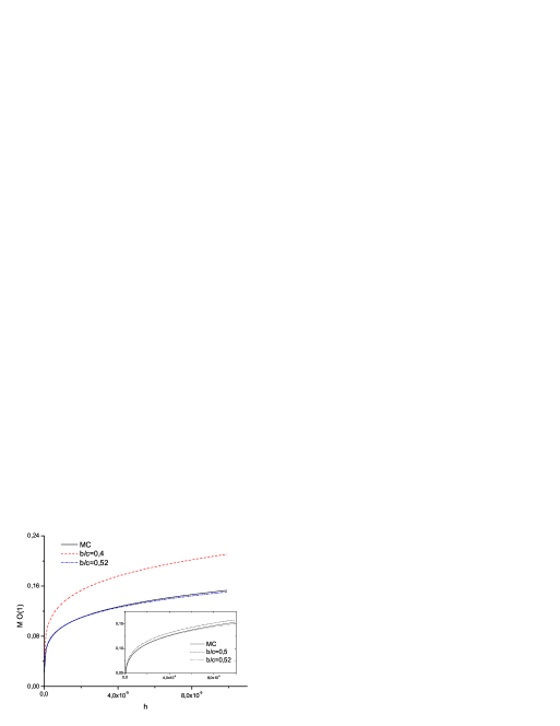
Figure 1: The dependence of the order parameter on the field for $\tau=0$ and n=1

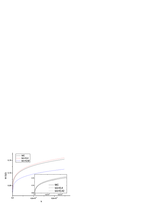
Figure 2: The dependence of the order parameter on the field for $\tau=0$ and n=2

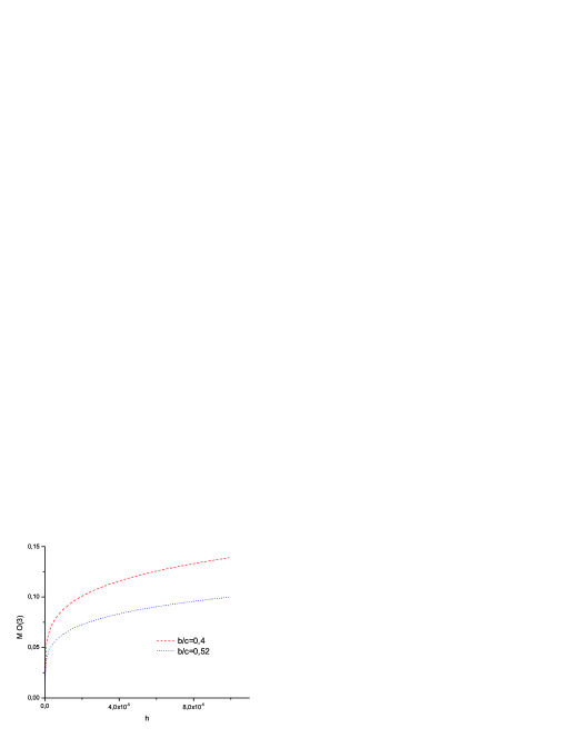
Figure 3: The dependence of the order parameter on the field for $\tau=0$ and n=3

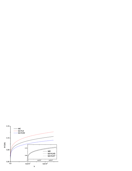
Figure 4: The dependence of the order parameter on the field for $\tau=0$ and n=4

There are different forms of the equation of state. Some discussion about convenience the correspondent forms of the equation of state is presented in 21 . The equation of state (101) can be reduced to the form used in Eng1 ; Eng2 ; Eng4 :

$$M=h^{1/\delta}f_{G}(z),$$ (104)

where:

$$h=H/H_{0},\;z=\frac{\bar{t}}{h^{\beta\delta}},\;\bar{t}=\tau\frac{T_{c}}{T_{0}},$$ (105)

and $f_{G}$ is the scaling function. The explicit form of $f_{G}$ can be found from extrapolation of the MC data obtained in Eng1 ; Eng2 ; Eng4 ; Camp . $H_{0}$ and $T_{0}$ are normalization constants. Such form is equivalent to the Widom-Griffiths equation of state Grif

$$y=f(x)$$ (106)

where

$$y\equiv h/M^{\delta},\;x\equiv t/M^{1/\beta}.$$ (107)

The scaling function obtained from Eq.(101) has the form

$$f_{G}=\left(s_{0}^{3/2}/h_{o}\right)^{\frac{1}{5}}\sigma_{00}\left(1+\alpha^{-2}\right)^{\frac{1}{10}}.$$ (108)

It depends on $\alpha$

$$\alpha=\frac{\tilde{h}}{\tilde{\tau}^{p_{0}}}.$$ (109)

The variables $\alpha$ and $z$ are connected with the ratio:

$$\alpha=\frac{s_{0}^{3/2}}{h_{o}}\left(\frac{f_{n}}{c_{1k}}\right)^{p_{0}}z^{-p_{0}},$$ (110)

that allows to compare our results with Monte-Carlo data. Figures 5-8 present graphs of the scaling functions for different n, where the dashed curve is the Monte-Carlo data.

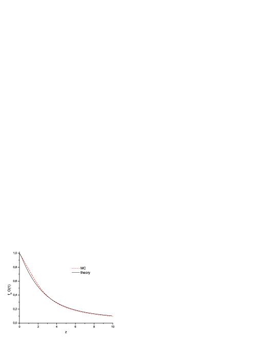
Figure 5: The scaling function for n=1 and $b/c=0.5$, solid curve – our results, dashed curve – Monte-Carlo data Eng1 .

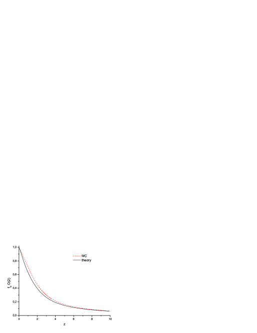
Figure 6: The scaling function for n=2 and $b/c=0.5$, solid curve – our results, dashed curve – Monte-Carlo data Eng2 .

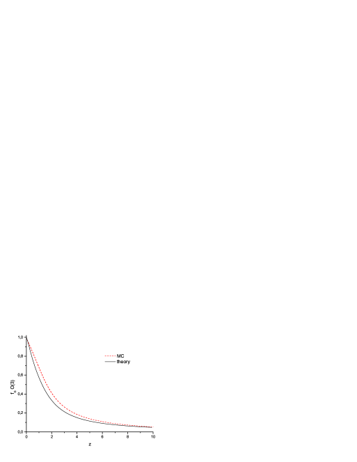
Figure 7: The scaling function for n=3 and $b/c=0.5$, solid curve – our results, dashed curve – Monte-Carlo data Camp .

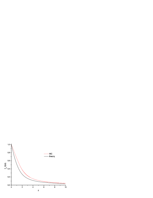
Figure 8: The scaling function for n=4 and $b/c=0.5$, solid curve – our results, dashed curve – Monte-Carlo data Eng4 .

V Conclusions.

We obtained the partition function of the n-vector model in the presence of the external field above the critical temperature by the CV method. The method of calculation corresponds to the general scheme of the RG approach. Taking into account the explicit form of the interaction potential allows to obtain the explicit dependence of the coefficients of the linearized recurrence relations on the temperature and the microscopic parameters of the model.

The explicit form of the exit point from the CR allows to obtain the equations for the recurrence relations in the CR suitable for any ratios of the temperature and the field. The structure of the partition function as a product of the partial partition functions that present different fluctuation processes allows to obtain the explicit form for the free energy of the system. The order parameter of the model was found by direct differentiation by the field.

The formulas to describe the field dependencies of the order parameter of the n-vector model with exponentially decreasing interaction potential for different ratios $b/c$ ($b$ is range of the interaction potential, $c$ is period of the simple cubic lattice) were obtained. It was found that for each value of n there is an appropriate value of $b$ for which our dependencies are close to Monte-Carlo data (see Fig.5-8).

The explicit form of the scaling function (108) was found. The comparison with Monte-Carlo data shows some difference for the behavior of $f_{G}(z)$ for intermediate values of $z$. It may be caused by used approximation in which the critical exponent $\eta=0$ and corrections to scaling were neglected. But further specification of calculations is a subject of a separate investigation.

VI Appendix

$$\varphi(x) = (n+2)U_{n}^{2}(x)+2xU_{n}(x)-2,$$

$$U_{n}(x) = \frac{U\left(\frac{n+1}{2},x\right)}{U\left(\frac{n-1}{2},x\right)},\;x=\sqrt{\frac{3}{a_{4}}}d(B_{1},B^{\prime}),$$

$U(a,x)$ is the function of Weber’s parabolic cylinder.

$$Q(d_{l}) = (2\pi)^{\frac{n}{2}}\left(\frac{3}{a_{4}^{(l)}}\right)^{\frac{n}{4}}U\left(\frac{n-1}{2},x_{l}\right)\exp\left({\frac{x_{l}^{2}}{4}}\right),$$

$$a_{4} = -3s_{0}^{d}\frac{n^{2}}{m^{4}}\left(1-z^{\prime}U_{n}(z^{\prime})-U_{o}^{2}\right),$$

$$U_{0} = \sqrt{\frac{n+2}{2}}U_{n}(z^{\prime}),\;z^{\prime}=\sqrt{\frac{3}{u^{\prime}_{4}}}u^{\prime}_{2},$$

$$r_{p+m} = \frac{U^{\prime}_{n}(x_{n_{p}+m})}{U_{n}(x_{n_{p}+m})}-\frac{1}{2}\frac{\varphi^{\prime}(x_{n_{p}+m})}{\varphi(x_{n_{p}+m})},$$

$$g_{p+m} = -\frac{\bar{x}E_{2}^{m-1}H_{cd}}{\sqrt{1+\Phi E_{2}^{m-1}H_{c}}}\left(1-\frac{H_{c}\Phi E_{2}^{m-1}}{2\left[1+\Phi E_{2}^{m-1}H_{c}\right]}\right),$$

$$\bar{x} = f_{n}\sqrt{\frac{3}{\phi_{n}}}$$

References

• (1) D. Bohm, General Theory of Collective Variables (Mir, Moscow, 1964) (in Russian).
• (2) D. N. Zubarev, Dokl. Akad. Nauk SSSR 95, 757 (1964) (in Russian).
• (3) I. R. Yukhnoskii, Phase Transitions of the Second Order. Collective Variables Method (World Scientific, Singapore, 1987).
• (4) K. G. Wilson, Phys. Rev. B 4, 3174 (1971).
• (5) A. Z. Patashinskii and V. L. Pokrovskii, Sov. Phys. JETP 23, 292 (1966).
• (6) L. P. Kadanoff, Physics 2, 263 (1966).
• (7) G. M. Avdeiva and A. A. Migdal, Sov. Phys JETP Lett. 16, 178 (1972) (in Russian).
• (8) E. Bresin, D. J. Wallace, and K. G. Wilson, Phys. Rev. Lett. 29, 591 (1972).
• (9) E. Bresin, D. J. Wallace, and K. G. Wilson, Phys. Rev. B 7, 232 (1973).
• (10) F. J. Wegner, Phys. Rev. B 5, 4529 (1972).
• (11) E. K. Riedel and F. J. Wegner, Phys. Rev. B 9, 1238 (1973).
• (12) M. E. Fisher and A. Aharony, Phys. Rev. B 10, 2818 (1974).
• (13) J. F. Nicoll and P. C. Albright, Phys. Rev. B 31, 4576 (1984).
• (14) D. R. Nelson, Phys. Rev. B 11, 3504 (1974).
• (15) C. Bagnuls and C. Bervillier, J. Phys. Lett. (Fr.) 45, L95 (1984).
• (16) V. Dohm, Z. Phys. B-Condensed Matter 60, 61 (1956).
• (17) H. J. Krause, R. Schloms, and V. Dohm, Z. Phys. B-Condensed Matter 79, 287 (1990).
• (18) Y. Okabe and K. Ohno, J. Phys. Soc. Jpn 53, 3070 (1984).
• (19) Y. Okabe and K. Ideura, Prog. Theor. Phys. 66, 1959 (1981).
• (20) E. Bresin, J. C. L. Guillon, and J. Zinn-Justin, Phys. Lett. A 47, 285 (1974).
• (21) A. M. Ferrenberg and D. Landau, Phys. Rev. B 44, 5081 (1991).
• (22) K. Chen, A. M. Ferrenberg, and D. P. Landau, Phys. Rev. B 48 (1993).
• (23) J. Engels, L. Fromme, and M. Seniuch, Nucl. Phys. B 655, 277 (2003).
• (24) J. Engels, S. Holtmann, T. Mendes, and T. Schulze, Phys. Lett. B 492, 219 (2000).
• (25) J. Engels and T. Mendes, Nucl. Phys. B 572, 289 (2000).
• (26) M. Campostrini, M. Hasenbusch, A. Pelissetto, P. Rossi, and E. Vicari, Phys. Rev. B 65, 40 (2002).
• (27) I. A. Vakarchuk, Y. K. Rudavskii, and Y. V. Holovach, Physics of Many Particle Systems 4, 44 (1983) (in Russian) .
• (28) I. R. Yukhnoskii, Selected works. Physics (Lviv Polytechnic National University, Lviv, 2005) (in Ukrainian).
• (29) Z. E. Usatenko and M. P. Kozlovskii, Phys. Rev. B 62, 3599 (2000).
• (30) Z. E. Usatenko and M. P. Kozlovskii, Mater. Sci. Eng., A 227, 732 (1997).
• (31) I. R. Yukhnovskii, M. P. Kozlovslii, and I. V. Pylyuk, Microscopic theory of phase transitions in the three-dimensional systems (Eurosvit, Lviv, 2001) (in Ukrainian).
• (32) M. P. Kozlovskii, Ukr. Fiz. Zh./Reviews (Ukr. ed.) 5, 61 (2009).
• (33) M. P. Kozlovskii, I. V. Pylyuk, and O. O. Prytula, Cond. Matt. Phys. 7, 361 (2004).
• (34) M. P. Kozlovskii, I. V. Pylyuk, and O. O. Prytula, Nucl. Phys. B 753, 242 (2006).
• (35) R. B. Griffiths, Phys. Rev. 158, 176 (1967).