Acoustic, thermal and flow processes in a water filled nanoporous glasses by time-resolved optical spectroscopy

Abstract

We present heterodyne detected transient grating measurements on water filled Vycor 7930 in the range of temperature $20-90~{}^{\circ}C$. This experimental investigation enables to measure the acoustic propagation, the average density variation due the liquid flow and the thermal diffusion in this water filled nano-porous material. The data have been analyzed with the model of Pecker and Deresiewicz which is an extension of Biot model to account for the thermal effects. In the whole temperature range the data are qualitatively described by this hydrodynamic model that enables a meaningful insight of the different dynamic phenomena. The data analysis proves that the signal in the intermediate and long time-scale can be mainly addressed to the water dynamics inside the pores. We proved the existence of a peculiar interplay between the mass and the heat transport that produces a flow and back-flow process inside the nano-pores. During this process the solid and liquid dynamics have opposite phase as predicted by the Biot theory for the slow diffusive wave. Nevertheless, our experimental results confirm that transport of elastic energy (i.e. acoustic propagation), heat (i.e. thermal diffusion) and mass (i.e. liquid flow) in a liquid filled porous glass can be described according to hydrodynamic laws in spite of nanometric dimension of the pores. The data fitting, based on the hydrodynamic model, enables the extraction of several parameters of the water-Vycor system, even if some discrepancies appear when they are compared with values reported in the literature.

I Introduction

The study of transport phenomena in heterogenous media is a fundamental issue of the material science Torquato (2006); Sheng (2006), its relevance spans from the basic physics (i.e. the proper definition of the equations of motion describing the transport processes) to the more recent technological applications. During the recent years, these studies have to face the scaling down of heterogeneity towards the nano-metric dimension.

Between the numerous random heterogenous media the two phase solid-liquid materials represent one of the most investigated. A large impulse, to these studies, has been given by the petroleum industry aimed at understanding the transport phenomena in sediment sands and porous rocks. In the basic research, probably the most studied materials are the solid porous matrix filled by a molecular liquid (e.g. liquid filled porous glasses), since typically they are well parameterized systems.

A part from the electric processes, three main transport phenomena are generally to be considered in the solid-liquid heterogenous materials: propagation of acoustic waves, thermal diffusion and viscous flow (i.e. transport of elastic energy, heat and mass). These phenomena are generally characterized by very different time/frequency scales so that often they have been considered as quasi-independent processes, both from the experimental and theoretical point of view. Moreover, they can be surprisingly described by relatively simple hydrodynamic models.

The propagation of sound in the liquid-filled porous materials has been described by phenomenological models based on hydrodynamic/elastic equations for the liquid/solid phases. The first model has been introduced by M. A. Biot in an important theoretical work in 1956 Biot (1956a, b). An extraordinary result of the Biot theory is the prediction of a new slow longitudinal wave besides the usual longitudinal and transverse waves. This wave has a velocity lower than the one of the bulk liquid Plona (1980); Smeulders (2005). In a recent experimental work the validity of this model in the high frequency range has been investigated Taschin et al. (2008a); Cucini et al. (2007), measuring the hypersonic sound propagation in a nano-porous media.

The viscous flow of liquids through porous media has always been a subject of intense study Bear (1972). Many studies have been concerned with the check of the validity of the macroscopic law of Darcy. Although Darcy’s law was determined phenomenologically, it is a direct result of the Navier-Stokes hydrodynamic equations Neuman (1977), thus checking its validity is a straightforward analysis of the hydrodynamical character of liquid flowing. Darcy’s law is shown to be valid for a wide range of porous media from porous rocks, sands Bear (1972) and glass beads Chandler (1981) whose heterogeneities are micrometric, up to porous glasses like Vycor which have heterogeneities of the order of few nanometers Debye and Cleland (1959); Lin et al. (1992); Li (2000); Vichit-Vadakan and Scherer (2000, 2008). Recently, many experimental and simulation works aimed at understanding to what extent the Navier-Stokes equation can describe the liquid flow at decreasing of the confinement size Travis et al. (1997); Spohr et al. (1999); Li (2000); Huang et al. (2007).

The thermal conductivity of heterogenous media is a complex problem which has to be characterized in a general theoretical framework Torquato (2006). The prediction of the effective permeability of saturated porous media remains, despite of many experimental and theoretical works, an unsolved problem in heat transfer science. In particular this quantity depends, as well as on macroscopic parameters of the two constituent phases, also on the particular morphology of the porous material which is in general experimentally not accessible. Nevertheless, the theory is able to fix the limits of the effective conductivity and give several approaches for calculating this quantity in particular kind of porous media Aichlmayr and Kulacki (2006).

Though the transport phenomena in liquid-filled porous glasses has been previously studied in the literature, many basic questions remain open. In our opinion, one of the more relevant is at which extent the hydrodynamic models are valid, especially when the media heterogeneity scale down versus molecular length scales.

We think that other experimental researches could infer new information, especially with techniques poorly applied in this field, like the time resolved spectroscopy experiments. Transient grating (TG) experiments Eichler et al. (1986); Yang and Nelson (1995) are powerful tools for investigate the relaxation dynamics of complex liquids Yang and Nelson (1995); Torre et al. (2001); Taschin et al. (2006); Taschin et al. (2008b), but only few previous experimental works utilized these techniques to investigate the porous glass samples Ritter et al. (1988); Taschin et al. (2007); Cucini et al. (2007); Taschin et al. (2008a). A particular kind of TG experiment offers the possibility to study, at one time, the acoustic propagation, the liquid flow and the thermal diffusion processes. The very broad time window covered by this experiment, typically from $10^{-9}$ to $10^{-3}~{}s$, gives access to a dynamic range hardly explored by other methods.

In this paper we present heterodyne detected transient grating (HD-TG) measurements on water filled Vycor nano-porous glass. The measured signal shows aspects related to the acoustic waves propagation, to the viscous liquid flow through pores, and, lastly, to the thermal diffusion. The transient grating experiment reported here is shown to be a powerful tool to measure the transport processes in liquid filled porous glasses.

To analyze the data we employ an hydrodynamic model introduced by Pecker and Deresiewicz Pecker and Deresiewicz (1973) which is a extention of the Biot’s theory Biot (1956a, b) to include the thermal effects. The model enables a safe and meaningful addressing of the different contributions present in the HD-TG signal, describing them on the base of few parameters characterizing the heterogenous system.

The present work is divided as follows. In Sec. II we report an overview of the TG experimental technique describing the involved excitation mechanisms and the measured dynamics with probing process. In Sec. III we present the experimental aspects of the work, laser systems, experiment optical set-up and the sample preparation. Section IV is devoted to the presentation of the data while the subsequent one to the introduction of the theoretical model used to analyze these data. Finally, in the last section we show the data analysis and we discuss the obtained results.

II Transient grating experiments

In a TG experiment, two infrared laser pulses, obtained dividing a single pulsed laser beam, interfere within the sample and produce an impulsive spatially periodic variation of the dielectric constant. The spatial modulation is characterized by a wave vector $\mathbf{q}$ which is given by the difference of the two pump wave vectors $\mathbf{k}_{1}-\mathbf{k}_{2}$ (see Fig. 1). Its modulus is $q=4\pi\sin(\theta_{ex})/\lambda_{ex}$, where $\lambda_{ex}$ and $\theta_{ex}$ are the wavelength and the incidence angle of the exciting pumps, respectively. The relaxation toward equilibrium of the induced modulation can be probed by measuring the Bragg scattered intensity of a second cw laser beam. The time evolution of the diffracted signal supplies information about the dynamic of the relaxing TG and, consequently, on the dynamical properties of the studied sample.

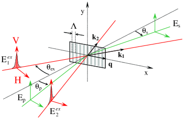
Figure 1: Schematic drawing of a transient grating experiment. Two excitation pulses, $E^{ex}_{1}$ and $E^{ex}_{2}$ induce an impulsive spatial modulation of the dielectric constant with step $\Lambda$. The relaxation of the induced transient modulation is probed by the Bragg scattering of a third beam, $E_{p}$.

TG experiments fall within the framework of the four-wave-mixing theory Shen (1984); Eichler et al. (1986); Taschin et al. (2008b); Hellwarth (1977). Under a few approximations, in particular, if the laser pulses do not have any electronic resonance with the material, it can be proved that the TG experiment can be divided in two separated processes: excitation and probing. Moreover, when the heterodyne detection is employed, the signal turns out to be directly proportional to the dielectric constant change induced by the pumps, $\delta\epsilon_{ij}$, or to the response function of the system, $R_{ijkl}$ Taschin et al. (2008b):

$$S^{HD}(q,t)\propto\delta\epsilon_{ij}(q,t)\propto R_{ijkl}(q,t)$$ (1)

where the cartesian indexes $i$ and $j$ define the polarizations of the diffracted and the probe fields, $k$ and $l$ define the polarizations of the pump fields. Both $\delta\epsilon_{ij}$ and $R_{ijkl}$ are spatial Fourier components corresponding to the exchanged wave vector $\mathbf{q}$, i. e. the grating wave vector. Hence, the heterodyne detected TG signal measures directly and linearly the relaxation processes defined by the tensor components of the response function. By selecting different polarizations of the fields, different elements of the response function tensor are probed. Generally, these elements can be different Taschin et al. (2001); Pick et al. (2004); Azzimani et al. (2007a, b). In materials, where the coupling between translational and rotational degrees of freedom is strong, the birefringence effects can be relevant and the TG signal will depend on the field polarization. When, instead, all the birefringence contributions are negligible, the signal turn out to be independent on the field polarization and the induced dielectric constant tensor is simple $I\delta\epsilon$, where $I$ is the identity tensor Taschin et al. (2008b).

Without birefringence effects and in bulk homogeneous materials, the transient grating is mainly induced by two effects. The electrostriction and the heating. The first effect arises from the interaction between the molecular dipoles induced by the pump fields and the same pump fields. The electrostriction produces a pressure grating and consequently a density grating launching two counter-propagating acoustic waves whose superposition makes a standing acoustic wave. The second exciting process arises from a weak absorption of the pump infrared radiation which is resonant with some vibrational states. The increasing of energy due to the pump absorption, generally, quickly thermalizes by fast non radiative channels and builds up a temperature grating. This one produces a pressure grating and then the pressure grating produces a density grating via thermal expansion. Now, besides acoustic waves, we have more a constant density grating supported by the temperature grating which relaxes by thermal diffusion. As we shall see in section IV, in a heterogeneous material the excitation sources are the same but the effects can be more complex.

III Experimental procedures

A detailed description of the lasers and the optical set-up of our TG experiment is reported in references Taschin et al. (2008b). Here we just recall the main aspects. A sketch of the TG optical set-up is reported in Fig. 2. The infrared pump pulses have a $1064~{}nm$ wavelength, a temporal length of $20~{}ps$ and repetition rate of $10~{}Hz$. They are produced by an amplified regenerated oscillator (Nd-YAG EKSPLA PL2143). The typically used pump pulse energy was $5~{}mJ$. The probing beam, instead, is a continuous-wave laser at $532~{}nm$ produced by a diode-pumped intracavity-doubled Nd-YVO (Verdi-Coherent). The two laser beams are collinearly sent to a phase grating (PG) to get the two pump pulses and the probe and local field beams. These are obtained taking the $+1$ and $-1$ diffraction orders of the infrared and green lasers. A couple of confocal achromatic lenses, AL1 and AL2, collects all the four beams and focuses them on the sample. The phase grating directly supplies a probe at the right Bragg angle and a local field exactly collinear with the scattered field and phase locked with the probe. The HD-TG signal is optically filtered and measured by a fast avalanche silicon photodiode with a bandwidth of 1 GHz (APD, Hamamatsu). The signal is then amplified by a DC-$800~{}MHz$ AVTECH amplifier and recorded by a digital oscilloscope with a $7~{}GHz$ bandwidth and a $20~{}Gs/s$ sampling rate (Tektronix). The instrumental function of our setup has a temporal full width half maximum of 1 $ns$ and is mainly determined by the bandwidth of the detector and its amplifier Taschin et al. (2008b).

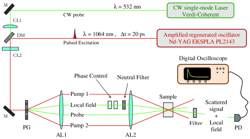
Figure 2: Optical set-up and laser system for the TG experiment with optical heterodyne detection. M are the mirrors; CL# the cylindrical lenses; DM a dichroic mirror; PG is the phase grating; AL# the achromatic lenses and PD is the photodiode.

Vycor 7930 is an open cell porous glass which is produced by a spinodal demixing in a borate-rich and borate-poor glass and subsequent bleaching of the borate-rich phase Cor . It has nominal values of porosity and mean pore size of $28\%$ and $4~{}nm$ respectively. The solid constituent of Vycor 7930 is the glass Vycor 7913 which is composed by $96\%$ of silica, by $3\%$ of boron oxide and the remaining part mostly by aluminum oxide and zirconium oxide. Our sample has been purchased from “Advanced Glass and Ceramics” in a cylindrical form, with a diameter of $15~{}mm$ and $10~{}mm$ thickness. In order to remove all the absorbed organic elements we washed the sample in $30\%$ water-hydrogen peroxide solution and then we heated it in a muffle up to $800~{}^{\circ}C$ at a rate of $0.3~{}K/min$. The sample has been kept at this temperature for several hours. Water has been obtained from a double-distilled water vial prepared for pharmaceutical purposes. The filled matrices were, then, placed in a thin teflon tube and closed between two circular quartz windows. The whole was inserted in a cylindrical copper cell (similar to the one reported in Halalay and Nelson (1990)). The holder was then stabilized in temperature with a stability of $\pm 0.1~{}K$.

IV Experimental Results

The HD-TG signals on water-filled Vycor have been collect in the range of temperature $20-90~{}^{\circ}C$ at different wave vectors. The data did not show a dependence on the polarizations of beams and consequently birefringence contributions were negligible Taschin et al. (2006). Hence, we recorded the data in a single configuration of beams polarization in which all the beams had a polarization perpendicular to the scattering plane as sketched in Fig. 1. The data at three different temperatures, 90, 40 and 20 ${}^{\circ}C$, are shown in Fig. 3 (following the usual TG signal convention, the sign of the data is chosen positive for a negative change of density Taschin et al. (2008b)).

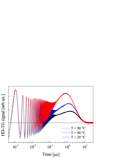
Figure 3: HD-TG data on Vycor-water system at $q=1~{}\mu m^{-1}$ at three different temperatures. At short times, the data show damped acoustic oscillations, at middle times, a density rearrangement related to liquid flow and finally, at long times, the data show a decay due to the thermal diffusion. The acoustic waves are practically induced only by the electrostrictive effect, while the remaining part of the signal by the thermal excitation.

Before explaining the data features, some considerations have to be discussed. As just mentioned in section II, in a TG experiment we have two exciting sources: the electrostrictive effect and the heating process. In the water filled Vycor, the first excitation is surely present in both materials, even if the electrostrictive strength could be different in the two materials, definitely we expect that this excitation source launches the acoustic waves. Differently, the heating should be much weaker in the solid part than in the liquid water or at the pore surfaces. In fact, the liquid water has a no negligible absorption coefficient at the pump wavelength and also the pore surfaces present a weak infrared absorption due to the presence of the silanol and boranol groups (Si-OH and B-OH). Nevertheless, on a very fast time scale, in the illuminated areas, all the sample components (solid part of the matrix, pore surfaces and liquid water) reach the same temperature. This makes applicable the assumption of local thermal equilibrium, i.e. we are supposing that the liquid and matrix temperatures are always locally equilibrated. Kaviany (Kaviany (1995) pp. 120-121) reports criteria of validity for the local thermal equilibrium approximation which are well fulfilled for the water-Vycor system. Namely, the approximation of local thermal equilibrium requires that the time scale associated with the inter-pore heat transfer must be much smaller than the time scale associated with the macroscopic heat transfer experimentally measured. The heat transfer between two pores occurs on a nanometric length scale while the macroscopic length scale is given by the spacing of the induced grating, $\Lambda=2\pi/q=6.28~{}\mu m$, for $q=1~{}\mu m^{-1}$. Moreover, the interphase heat transfer is a very efficient process thanks the very large specific pore surface area. We expect this process to evolve on shorter time scales than the time scales measured in the HD-TG signal. So, also in our heterogenous sample the pump heating produces an uniform temperature grating as in a bulk homogeneous sample.

Now, other important aspects have to be considered to understand the HD-TG signals: 1) the thermal expansion coefficient of the matrix is very low compared to the water one; 2) the bulk modulus of the matrix is higher than the water one, the matrix is stiff. Since the thermal expansion of water would be greater than that of the matrix, at first the expansion of the liquid is reduced by the stiffness of the matrix which exerts a pressure on the liquid. At later times, the liquid flows through the pores to nullify the matrix pressure which is at first positive and then negative, as it will be proved later using a data simulation based on the hydrodynamic model. So, the liquid can practically expand only via the flowing. This implies also that the acoustic oscillations induced by the temperature grating are characterized by a very low amplitude.

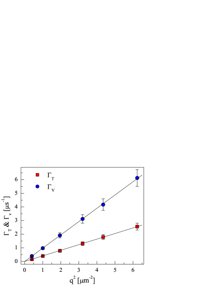
Figure 4: Decay constants of the two exponentials describing the long part of the signal as a function of $q^{2}$ at the fixed temperature of 30 ${}^{\circ}C$. $\Gamma_{V}=1/\tau_{V}$ and $\Gamma_{T}=1/\tau_{T}$ are, respectively, the decay constants of the exponential rise and fall of the signal. The linear behavior confirms the diffusive character of the viscous flow mode and of the thermal diffusion.

For the aforementioned reasons, the data show, at short times, damped acoustic oscillations induced almost only by the electrostrictive effect, at intermediate times, a density rearrangement related to liquid flow inside the pores.

From preliminary fits of the intermediate and long parts of the signals, we obtain that the rise is well reproduced by a single exponential whose time constant, $\tau_{V}$, shows a $q^{-2}$ dependence. It is, therefore, a diffusive mode and it turns to be the Biot slow wave in diffusive regime, as it will shown later using the hydrodynamic model. The time constant, then, is related to the constant diffusion of the Biot slow wave (hydraulic diffusivity coefficient) which is connected to Vycor permeability and liquid viscosity. Clearly, in this case the temperature grating plays an important role, it is the pumping source for the liquid motion. In Fig. 4 we report the inverse of constant times of the exponential signal rise, $\Gamma_{V}=1/\tau_{V}$, and the exponential signal fall, $\Gamma_{T}=1/\tau_{T}$, as a function of the $q^{2}$ for the temperature fixed at 30 ${}^{\circ}C$. The probed wave vectors were $q=0.63$, 1.00, 1.39, 1.76, 2.15, and 2.51 $\mu m^{-1}$. The linear behavior of the time constants confirms the diffusive character of the modes.

V Theoretical background

An explicit function of the TG signal can be obtained developing the dielectric function $\delta\epsilon$ through the hydrodynamic variables which, in the absence of birefringence effects, are only the density and the temperature. According to a first-order approximation, the dielectric constant change in a homogeneous bulk material is Berne and Pecora (1976):

$$\delta\epsilon(t)=\left(\frac{\partial\epsilon}{\partial\rho}\right)_{T}\delta\rho(t)+\left(\frac{\partial\epsilon}{\partial T}\right)_{\rho}\delta T(t),$$ (2)

Now we have to consider that our sample is composed by two interconnected materials, Vycor and water. The dielectric constant change will depend on two densities and two temperatures:

$$\delta\epsilon(t) =\left(\frac{\partial\epsilon}{\partial\rho_{1}}\right)_{T_{m},T_{l},\rho_{2}}\delta\rho_{1}(t)+\left(\frac{\partial\epsilon}{\partial\rho_{2}}\right)_{T_{m},T_{l},\rho_{1}}\delta\rho_{2}(t)$$ (3)

$$+\left(\frac{\partial\epsilon}{\partial T_{m}}\right)_{T_{l},\rho_{1},\rho_{2}}\delta T_{m}(t)+\left(\frac{\partial\epsilon}{\partial T_{l}}\right)_{T_{m},\rho_{1},\rho_{2}}\delta T_{l}(t)$$

where $\rho_{1}=(1-\phi)\rho_{s}$ and $\rho_{2}=\phi\rho_{l}$ are the average densities of matrix and water respectively, in which $\phi$ is the porosity of Vycor, $\rho_{s}$ the density of solid and $\rho_{l}$ the water density. $T_{m}$ and $T_{l}$ are the matrix and water temperatures respectively. The dielectric constant change induced directly by the temperature variation, in Eq. (2), is generally neglected in the TG signal analysis because for most of liquids $(\partial\epsilon/\partial T)_{\rho}\delta T$ is much lower than $(\partial\epsilon/\partial\rho)_{T}\delta\rho$. Water is an example for which this condition is not satisfied, and the TG signal depends also on this contribution Taschin et al. (2006). Thus, we can neglect the matrix temperature contribution, but not the water temperature contribution that could have an important weight:

$$\delta\epsilon(t)=\left(\frac{\partial\epsilon}{\partial\rho_{1}}\right)\delta\rho_{1}(t)+\left(\frac{\partial\epsilon}{\partial\rho_{2}}\right)\delta\rho_{2}(t)+\left(\frac{\partial\epsilon}{\partial T_{l}}\right)\delta T_{l}(t)$$ (4)

The previous equation can be rewritten in the following way:

$$\delta\epsilon(t)=\left(\frac{\partial\epsilon}{\partial\rho_{2}}\right)\left[A_{12}\delta\rho_{1}(t)+\delta\rho_{2}(t)+E\frac{\rho_{2}}{T_{0}}\delta T_{l}(t)\right]$$ (5)

where we have defined

$$A_{12}=\frac{\left(\partial\epsilon/\partial\rho_{1}\right)}{\left(\partial\epsilon/\partial\rho_{2}\right)}\quad and\quad E=\frac{T_{0}\left(\partial\epsilon/\partial T_{l}\right)}{\rho_{2}\left(\partial\epsilon/\partial\rho_{2}\right)}$$ (6)

$A_{12}$ and $E$ are amplitude parameters which define the relative weight between the three different contributions in the final signal. $E$ is defined similarly in Taschin et al. (2006), but its value could be different from that measured for the bulk water because of the strong interactions between water molecules and the hydrophilic surfaces of Vycor pores. This interaction strongly modifies the hydrogen bonds among water molecules and it could change the value of $E$. Thus, both the parameters, $A_{12}$ and $E$ must be valued from the data fitting.

V.1 Hydrodynamic model

The time evolution of the two densities and the two temperatures can be obtained from the thermo-poroelastic model introduced in 1973 by Pecker and Deresiewicz (P-D)  Pecker and Deresiewicz (1973). This is an extension of the well known Biot model on the wave propagation on poroelastic system to account for the temperature effects. An earlier attempt to include the temperature was made by Zolotarev in 1965 Zolotarev (1965), but here strong approximations were introduced. The model of Pecker and Deresiewicz has been later deeply revisited as linearized approximation of more complex models by Gajo Gajo (2002) and Youssef Youssef (2007). We shall follow here the Pecker and Deresiewicz (P-D) model adopting the same notation since exactly alike to the Biot one.

The main assumptions of the theory are the same of the Biot theory. In particular: the solid phase of the system is perfectly elastic, homogeneous and isotropic; the liquid is a compressible perfect fluid; the liquid viscosity is only introduced into a dissipation function to account for the sound wave attenuations due to the viscous friction between matrix and liquid; sound wavelengths are much larger than the heterogeneity dimensions; finally, all the transformations (displacements, strains, etc.) are considered infinitesimal in order to obtain a linear theory.

In comparison with Biot model, two relaxation equations are added for the matrix and liquid temperatures and some thermo-mechanical coupling terms are inserted in all the equations to account for the coupling effects between the two temperatures and the two densities.

Since in an isotropic medium TG experiment is sensible only to density and temperature changes, we focus our attention only to the motion equations of the matrix and liquid dilatations discarding the shear motions.

Defining with $\mathbf{u}$ and $\mathbf{U}$ the displacements of solid and liquid phases Landau and Lifshitz (1959), the dilatations are defined by $e=\mathbf{\nabla}\cdot\mathbf{u}$ and $\mathcal{E}=\mathbf{\nabla}\cdot\mathbf{U}$. $e$ and $\mathcal{E}$ are related to the matrix and liquid density changes, $\delta\rho_{1}$ and $\delta\rho_{2}$, by the following identities:

$$\delta\rho_{1}=-\rho_{1}e\quad and\quad\delta\rho_{2}=-\rho_{2}\mathcal{E}$$ (7)

The time evolution of the dilatations $e$ and $\mathcal{E}$ and the temperature variations $\delta T_{m}$ and $\delta T_{l}$ can be evaluated by the P-D model. In the appendix we report the detailed description of the P-D equations and all the expression of the coefficients. Few approximations suitable for the water-Vycor system can be made to this model (see appendix), in particular we can assume the local thermal equilibrium by which the liquid and matrix temperatures can be always considered locally equilibrated: i.e. $T_{m}=T_{l}=T$. After that, the linearized P-D equations in the Fourier q-space become:

$$\rho_{11}\ddot{e}+\rho_{12}\ddot{\mathcal{E}}+b(\dot{e}-\dot{\mathcal{E}})+q^{2}Pe+q^{2}Q\mathcal{E}-q^{2}R_{1}\delta T=0$$

$$\rho_{12}\ddot{e}+\rho_{22}\ddot{\mathcal{E}}-b(\dot{e}-\dot{\mathcal{E}})+q^{2}Qe+q^{2}R\mathcal{E}-q^{2}R_{2}\delta T=0$$

$$F\dot{\delta T}+R_{1}T_{0}\dot{e}+R_{2}T_{0}\dot{\mathcal{E}}+q^{2}k\delta T=0$$ (8)

where the densities $\rho_{ij}$ are related to the solid and liquid densities, $\rho_{s}$ and $\rho_{l}$, by $\rho_{11}=(1-\phi)\rho_{s}-\rho_{12}$, $\rho_{22}=\phi\rho_{l}-\rho_{12}$ and $\rho_{12}=(1-\tau)\phi\rho_{l}$ where $\tau$ is the tortuosity of the matrix Biot (1956a, b). The $b(\dot{e}-\dot{\mathcal{E}})$ is a viscous friction term arising from the relative motion between the two materials, being $b=\phi^{2}\mu_{l}/k_{D}$, with $\mu_{l}$ the water dynamic viscosity and $k_{D}$ the Vycor permeability. This term is, at the same time, the damping source for the acoustic waves and the hindrance to the liquid slow flow through pores. $P$, $Q$ and $R$ are the generalized isothermal elastic moduli, the coefficients $R_{i}$ are the generalized expansion coefficient and the $F$ coefficient is a generalized specific heat Biot (1956a, b); Johnson (1982); Carcione (2001). $k$ is the effective thermal conductivity. The complete definition of these coefficients is reported in appendix. These equations enable to calculate the $q$-component of the time dependent variables $e$, $\mathcal{E}$ and $\delta T$, and thus, using the equations  1,  5 and 7, to simulate the measured signal.

The model of P-D model is an extension of Biot’s model in the low frequency limit, i.e. is valid for motions at frequencies lower than the Biot characteristic frequency. This quantity is defined by $f_{c}=\mu_{l}/\pi\rho_{l}r^{2}$ with $r$ the mean pore radius of the matrix. For the water-Vycor system the characteristic frequency is $26-80~{}GHz$ in the temperature range considered. This value has to be compared to the higher frequency experimentally excited which is almost 0.6 $GHz$ (the experimental frequency can be obtained by $f=cq/2\pi$ where $c=4~{}Km/s$ is the measured sound velocity and $q=1~{}\mu m^{-1}$ the exchanged wave vector). Thus, our experiment is testing dynamics at frequencies always lower then $f_{c}$ and the present model is theoretically suitable to describe our signals. Moreover, when the involved frequency is much lower than the characteristic frequency, the dependence on the tortuosity, $\tau$, of the solutions of Eq.s (26), should be negligible. This condition has been verified in our case by the fitting procedure. As final consideration, we want to stress that the above equations, and consequently their solutions, do not depend explicitly on the pore dimension. Nevertheless, this parameter enters in the definition of the characteristic frequency, thus, fixing the applicability limit of the theory.

V.2 TG response and signal

The set of Eq.s (8) can be reduced to a first order differential equation system by introducing two additional variables $\psi_{1}=\dot{e}$ and $\psi_{2}=\dot{\mathcal{E}}$. The set of equations (8) can, thus, be easily written in the compact form

$$\dot{\mathbf{X}}(t)=-\mathbf{M}\cdot\mathbf{X}(t)$$ (9)

where $\mathbf{X}=(e,\mathcal{E},\psi_{1},\psi_{2},\delta T)$ and M is a matrix of coefficients which can be easily obtained from Eq.s (8). Indeed we can solve the system by diagonalizing, with standard routines, the non symmetric $\mathbf{M}$ matrix, i.e. $\mathbf{M}\cdot\mathbf{V=V}\cdot\mathbf{D}$ where $\mathbf{D}$ is diagonal and the resulting time solution is written as

$$\mathbf{X(}t\mathbf{)=V}\cdot\exp(-\mathbf{D\ }t\mathbf{)\cdot}\left[\mathbf{V}^{-1}\cdot\mathbf{X}(0)\right]$$ (10)

We note that it is possible to avoid the $\mathbf{V}$ matrix inversion, since $\mathbf{Y=V}^{-1}\cdot\mathbf{X(}0\mathbf{)}$ is the solution of linear system $\mathbf{V}\cdot\mathbf{Y=X(}0\mathbf{)}$. We want to stress that only the elements of the amplitude matrix, $\mathbf{V}$, and the root matrix, $\mathbf{D}$, need to be numerically calculated. Each element of the solution vector $\mathbf{X}(t)$ is a sum of two oscillating terms, cosine and sine rising from the two complex and conjugate roots of $\mathbf{D}$, and three pure exponential terms deriving from the other three real roots of $\mathbf{D}$.

The temporal expressions of the dilatations and the temperature must be calculated considering that the electrostriction produces a non zero initial condition on $\psi_{1}$ and $\psi_{2}$ and the heating produces a no null initial condition on $\delta T$: $\mathbf{X}(0)=(0,0,\psi_{1}(0),\psi_{2}(0),\delta T(0))$. These solutions together with the expressions for the densities (7) and the expression for dielectric constant change (5) give the signal function:

$$S^{HD}(t)\propto\delta\epsilon(t)= Ae^{-t/\tau_{S}}cos(\omega_{S}t)+Be^{-t/\tau_{S}}sin(\omega_{S}t)+$$ (11)

$$Ce^{-t/\tau_{1}}+De^{-t/\tau_{2}}+Fe^{-t/\tau_{3}}$$

where the amplitudes $A$, $B$, $C$, $D$, and $F$, the acoustic parameters $\tau_{S}$ and $\omega_{S}$, and the time constants $\tau_{1}$, $\tau_{2}$, and $\tau_{3}$ are functions depending on all the hydrodynamic parameters appearing in the starting equations and on the initial conditions and need to be numerically calculated at changing of the fitting parameters listed below.

The oscillating terms in Eq. (11) accounts for the induced acoustic oscillations and the three exponentials for the remaining part of the signal. As previously discussed, the acoustic oscillations induced by the temperature grating are partially prevented. Anyhow, these ones have been equally considered in the fitting analysis and they proved to be very small at all the temperatures, around 5$\%$ of those induced by the electrostriction.

Finally, Eq. (11) with the addition of electronic response function and convoluted with the experiment instrumental function, yields the used fitting function Taschin et al. (2008b).

VI Data analysis and discussion

The literature provides many of the water and Vycor data appearing in the P-D equations: the densities $\rho_{s}$, $\rho_{l}$, the expansivities $\alpha_{s}$, $\alpha_{l}$, the water viscosity $\mu_{l}$, the specific heats $C_{ps}$, $C_{pl}$, the Vycor porosity $\phi$, the transverse and longitudinal sound velocities of solid constituent for the calculus of $K_{s}$ and the adiabatic sound velocity of water and the specific heat ratio $\gamma_{r}$ for the calculus of $K_{l}$.

The other parameters were free fitting parameters. In table 1 we list the parameters locked to the literature values with the corresponding references.

As reported in Sec. III, the solid constituent of Vycor 7930 is not pure silica but Vycor 7913, a mixture of $96\%$ of silica and $3\%$ of boron oxide. Corning company Cor supplies us all the parameters of interest of Vycor 7913 only at room temperature. To overcome this problem, we made the hypothesis that the thermodynamic parameters of Vycor 7913 follow the temperature dependence as in silica Scopigno (2001). Considering the restricted range of temperature analyzed, this is surely a valid approximation.

For the calculation of the shear and bulk moduli of dry matrix, we take the matrix longitudinal sound velocity as free fitting parameter and the transverse sound velocity proportional to the longitudinal one as in the solid phase: $V_{t,m}=0.62V_{l,m}$ where the $m$ and $s$ indices refer to the matrix and solid materials and $l$ and $t$ to the longitudinal and transverse wave mode respectively Terki et al. (1998); Caponi et al. (2002); Levelut and Pelous (2007).

As porosity, we use the value of $31\%$, which is the mean of values reported in the literature Debye and Cleland (1959); Vichit-Vadakan and Scherer (2000, 2008); Gille et al. (2002).

In reference Taschin et al. (2008a) we proved that the Biot theory is not able to predict the acoustic damping times of TG data giving far overestimated values. The reason, probably, lies in the only damping mechanism considered in the theory, i.e. the energy dissipation due to the viscous friction between the matrix and liquid. Other damping effects, like the intrinsic dissipation of two materials are not included. P-D model does not introduce substantial modifications for the wave propagation and retains the same limitations of the Biot model. In order to avoid that the extraction of other interesting parameters could be affected by this mismatch, we multiply the oscillating terms of the solution (11) by $e^{-t/\tau_{A}}$ to account for the real exponential decay of the acoustic waves.

Finally, the free fitting parameters were: the three initial conditions $\psi_{1}(0)$, $\psi_{2}(0)$ and $\delta T(0)$, the relative amplitudes $E$ and $A_{12}$, the longitudinal sound velocity of the matrix $V_{l,m}$, the acoustic damping time $\tau_{A}$, the permeability $k_{D}$ and, lastly, the effective thermal conductivity $k$. This last parameter could to be fixed to the value given by the expression used in the the P-D model $k=(1-\phi)k_{s}+\phi k_{l}$, where $k_{s}$ and $k_{l}$ are the solid and liquid thermal conductivity, respectively. According to our data fitting, this value turned out not to be correct and we were forced to leave it free.

Table 1: Water and Vycor parameters fixed in the fitting procedure to the values found in the corresponding references.

Symbol	Definition	Values @ 20$~{}^{\circ}C$	Ref.
$\rho_{s}$	solid density	$2180$ $Kgm^{-3}$	Cor
$\rho_{l}$	water density	998 $Kgm^{-3}$	Weast and Lide (1989-1990)
$\alpha_{s}$	linear solid expansivity	$7.5\times 10^{-7}$ $K^{-1}$	Cor
$\alpha_{l}$	volume water expansivity	$2.07\times 10^{-4}$ $K^{-1}$	Weast and Lide (1989-1990)
$\mu_{l}$	water viscosity	$10^{-3}$ $Pa\cdot s$	Weast and Lide (1989-1990)
$C_{ps}$	solid specific heat	$739$ $JK^{-1}Kg^{-1}$	Lord and Morrow (1956)
$C_{pl}$	water specific heat	$4184$ $JK^{-1}Kg^{-1}$	Weast and Lide (1989-1990)
$\phi$	porosity	$31\%$	Debye and Cleland (1959); Vichit-Vadakan and Scherer (2000, 2008); Gille et al. (2002)
$V_{l,s}$	solid longitudinal sound velocity	5779 $ms^{-1}$	Cor ; Scopigno (2001)
$V_{t,s}$	solid transverse sound velocity	3580 $ms^{-1}$	Cor ; Scopigno (2001)
$V_{l}$	water adiabatic sound velocity	1483 $ms^{-1}$	Nis
$\gamma_{r}$	water specific heat ratio	1.0065	Nis ; Johari et al. (1996)

The used fitting function is able to reproduce the data in all temperature range analyzed. In the left panel of Fig. 5 we report in semi-log scale the fit-data comparison of the signal at 20 ${}^{\circ}C$ together with the corresponding discrepancy. In the right panel of the same figure, we show in linear scale the same fit-data comparison, together with the three different contributions appearing in expression (5). These are the matrix density contribution (green line), the water density (blue line) and the temperature one (orange line) contributions. The sum of these three contributions gives the shown fitting curve. As clearly visible, the water density change is the main term and it is the only one yielding the bump in the signal. Thus, the long time dynamics is mainly related to the water density changes and this is clearly due to the great difference between the water and Vycor expansivities and to the stiffness of the matrix. The signal contribution induced directly by the temperature (third term of Eq. 4, $\left({\partial\epsilon}/{\partial T_{l}}\right)\delta T_{l}(t)$) is practically described by a single exponential decay, it does not show any acoustic oscillation and has an intensity weakly dependent on the temperature. We want to stress that, as regards the acoustic oscillations, the liquid and matrix move in phase (see the inset of Fig. 5). Contrary, in the major part of the signal the water and matrix densities have opposite derivatives, i.e. when the liquid tends to expand the matrix tends to compress and vice versa. This implies an out-phase motion of the liquid and matrix as expected for the slow sound predicted by the Biot theory.

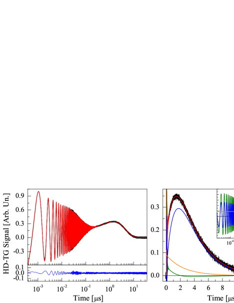
Figure 5: Comparison between data (black line) and fit (red line) for the temperature $20~{}^{\circ}C$ with the relative discrepancy (left panel). In the right panel the three different contributions whose sum gives the fit of the datum at $20~{}^{\circ}C$ are shown. These are the matrix density contribution (green line), the water density (blue line) and the temperature (orange line) contributions. The inset shows the same contributions in x-log scale.

Once we extracted all the parameters for a given temperature, we can use them to simulate the time dependence of an isolate physical observable. It is interesting to study the temporal behavior of the liquid pressure inside the pores. This can be obtained from the constitutive equation for the pore fluid Pecker and Deresiewicz (1973):

$$\delta p(t)=-\frac{1}{\phi}[Qe(t)+R\mathcal{E}(t)-(R_{1}+R_{2})\delta T(t)]$$ (12)

Figure 6: Temporal evolution of the pore pressure obtained from the constitutive equations for the pore fluid (Eq. 12) using the parameters extracted by the fit of the datum at 20 ${}^{\circ}C$. The pressure shows two relaxation modes, a fast one which drives the acoustic oscillations (inset in the figure) and a slow one which drives the liquid motion inside the pores.

Figure 6 shows the temporal evolution of the pore pressure change calculated with the parameters of the fit at 20 ${}^{\circ}C$. It is interesting to note that the liquid pressure change is never equal to zero (apart when it changes sign) during the signal evolution. This behavior is different from what appears in a bulk liquid sample where the pressure equilibrates after the vanishing of the acoustic oscillations. In the case of confined water, the liquid expansion due to the heating is partially prevented by the stiffness of the matrix which exerts a pressure on the liquid. At first, the liquid will change its density via the outflow from the heated pores to nullify this pressure. At later times, owing to the vanishing of the thermal grating for thermal diffusion, the matrix will exerts a negative pressure on the liquid which backflows to the pores to equilibrate again the pressure. Thus, density changes related to the liquid flow take place on time scales much longer and the liquid pressure is different from zero at all the times. Finally, the liquid pressure shows two relaxations, a fast one which drives the acoustic oscillations (the fast Biot wave) and a slow one which drives the liquid motion inside the pores (the slow Biot diffusive wave).

VII Fitting Results

In this last section, we shall show and discuss the main findings derived by the fit-data analysis. We will start with the results of acoustic wave propagation after that we will analyze the features connected with liquid viscous flow and finally with the thermal diffusion.

As already said in previous section, many of the parameters appearing in the equations of P-D model have been kept fixed to the literature values. These values are, clearly, measured for the bulk materials. For the case of water the assumption to consider the thermodynamic and dynamic parameters of confined water equal to the bulk ones is not so obvious. The strong hydrogen bonds of water molecules with the silanol groups of the inner pore surfaces of Vycor could affect parameters like the density, specific heat, viscosity, thermal expansivity, etc. For example, it has been found by molecular simulation Gallo et al. (2000) that the density of water confined in Vycor is around $11\%$ lower than the bulk value. Yet, the specific heat has been measured $1-2\%$ higher than in the bulk Tombari et al. (2005). Contrary, measurements of viscosity of water confined in nanometer films proved that this parameter remains close to the bulk value Raviv et al. (2001, 2004). Nevertheless, the data about the thermodynamic parameters of water in confined state are few and, in particular, no data about their temperature evolution exist. For this reason, we have chosen to fix the values of these parameters to the bulk ones as it has been done so far in all the experimental study on confined water.

In Fig. 7 we report the temperature behavior of the longitudinal sound velocity of Vycor $V_{l,m}$. We were forced to leave this parameter as free fitting parameter in order to have a good fit of acoustic oscillations at all the temperatures. These values together with the transverse velocity values, $V_{t,m}=0.62V_{l,m}$, and the values of matrix density, give the matrix stiffness values which differs from the those measured by static experiments Vichit-Vadakan and Scherer (2000, 2008); Cor . But our longitudinal sound velocities are in reasonable agreement with the values measured by Brillouin scattering experiments by Levelut and Pelous Levelut and Pelous (2007).

Figure 7: Longitudinal sound velocity of vycor as a function of temperature.

Figure 8: Measured acoustic attenuation times (circles) compared with the values predicted by the model of Pecker and Deresiewicz (continuous line).

In Fig. 8 we show the measured acoustic attenuation times compared to the prediction of the P-D model. We see that the times predicted by the theoretical model are much longer than the experimental ones and moreover their temperature behavior show an opposite trend. As stated before, P-D model does not introduce substantial modifications for the wave propagation and retains the same limitations of the Biot model. As just reported in Taschin et al. (2008a), the only damping mechanism considered in the theory (the energy dissipation due to the viscous friction between the matrix and liquid) is not surely the main damping source in Vycor filled with liquids at our TG frequencies. Other damping effects should be included, beginning with the dissipation phenomena intrinsic of the Vycor and water. Considering the very low sound attenuation in bulk water, the damping could be mainly due to the sound damping in Vycor. Indeed, the underestimations of the damping mechanism has been already reported in the literature Dvorkin and Nur (1993); Kibblewhite (1989); Williams et al. (2002).

In Fig. 9 we show the measured permeability $k_{D}$ as a function of temperature. $k_{D}$ does not show, within the experimental errors, a temperature dependence and has a mean value of $\sim 0.126~{}nm^{2}$. The permeability is related to the viscous Darcy coefficient $b=\phi^{2}\mu_{l}/k_{D}$ and to the hydraulic diffusivity coefficient Smeulders (2005): $D_{H}=(PR-Q^{2})/[b(P+R+2Q)]$, being $P$, $Q$ and $R$ the generalized elastic moduli defined in the appendix. In fact, the P-D model is an hydrodynamical theory that supposes that the flow of liquid through the pores is a Darcy flow (i.e. that the flow is laminar and the fluid velocity at pore wall is zero). This is assumed in the definition of the dissipative force $b(\dot{e}-\dot{\mathcal{E}})$ and, in particular, in the expression of $b$. In this model, the permeability of the porous material, $k_{D}$, is a quantity depending only on the geometrical characteristics of the porous material, porosity, mean pore size and tortuosity. Indeed the $k_{D}$ values extracted by the fit does not show any appreciable temperature dependence.

The value of the measured permeability can be compared with that of reference Vichit-Vadakan and Scherer (2000, 2008) ($k_{D}=0.065~{}nm^{2}$) and with that calculated following the expression of the Poiseuille permeability for a porous medium Guo et al. (1994): $k_{D}=(1/8)r^{2}\phi/\tau$ where we recall $r$ and $\tau$ are the mean pore radius and the tortuosity of the medium. By inserting the value of $31\%$ for the porosity and of $2~{}nm$ for the mean pore radius, supplied by the Corning company, and a tortuosity value of 2-4 Lin et al. (1992); Vichit-Vadakan and Scherer (2000, 2008), we find a permeability of $0.04-0.08~{}nm^{2}$. Thus, our $k_{D}$ fitting values do not agree with the previous reported measurements. This could be ascribed to a mean pore size larger than what stated by the company. Frequently in literature, measured values of porosity and mean pore size have been found different from the usual Corning values. For example, in ref. Vichit-Vadakan and Scherer (2000, 2008), it is reported a mean pore radius of $2.68~{}nm$ in Li (2000) of $2.3~{}nm$. Our results would be compatible with a mean pore radius around $3~{}nm$.

Figure 9: Permeability of water in Vycor extracted from the fits.

In Fig. 10 we report the temperature behavior of the measured effective thermal conductivity, $k$. We report also the values of the thermal conductivities calculated according to the weighted on porosity arithmetic mean (red line), $k=(1-\phi)k_{s}+\phi k_{l}$, and harmonic mean (blue line), $1/k=(1-\phi)/k_{s}+\phi/k_{l}$, being $k_{s}$ the solid thermal conductivity equal to $1.29$ $Wm^{-1}K^{-1}$ @ $20~{}^{\circ}C$ and $k_{l}$ water thermal conductivity equal to $0.60$ $Wm^{-1}K^{-1}$ @ $20~{}^{\circ}C$ Weast and Lide (1989-1990). These expressions of the effective conductivity refers to a medium composed by parallel layers of solid and water where the heat transfer goes along the layer direction (parallel conduction) or goes perpendicular to the layer direction (series conduction) Aichlmayr and Kulacki (2006). The value of these two values can be considered as the two limiting values of the $k$ parameter, see also appendix. The values obtained by our fitting is in substantial agreement with the harmonic mean.

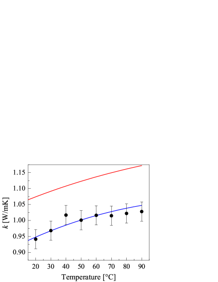
Figure 10: Effective thermal conductivity as a function of temperature compared with the maximum theoretical values (red line) and the minimum ones (blue line).

Finally, we want to show the results obtained for the amplitude parameters $E$ and $A_{12}$. These are shown in Fig. 11. Both the parameters do not show, within the experimental error bars, a sensible temperature dependence. In the same figure, the $E$ values are compared with the ones obtained for the bulk water Taschin et al. (2006). Unfortunately, we have not enough sensibility to estimate if and how the confinement affects the photothermal effect of water. Anyway, we want to underline that both the matrix and temperature contributions are absolutely necessary to describe correctly the data.

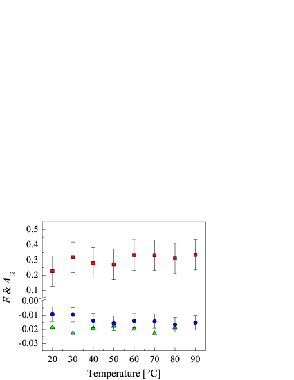
Figure 11: Temperature behavior of the parameters $E$ (blue circles) and $A_{12}$ (red squares). Green triangles refer to the $E$ values measured in the bulk water Taschin et al. (2006).

Considering the complexity of the fitting model, the agreement of the P-D parameters with the literature data is reasonable even if it is not complete. Correction on some fixed parameter could lead probably to a better agreement. In particular, possible changes of the water parameters due to the confinement should be taken in to account. Nevertheless, the fact that the model is able to reproduce the data at all the temperatures with a substantially small number of free parameters catching the main temperature dependencies and the order of magnitude of the coefficient values, proves the overall validity of the hydrodynamic laws in describing an nano-heterogenous system.

VIII Conclusions

In summary, heterodyne detected transient grating experiment has been applied to study the relaxation dynamic of water confined in Vycor 7930. We acquired HD-TG data in the temperature range $20-90$ ${}^{\circ}C$ at the q-vector of 1 $\mu m^{-1}$ and for the range of $q=0.63-2.5$ $\mu m^{-1}$ at 30 ${}^{\circ}C$. The HD-TG experiment enables to investigate in a single data the damped acoustic oscillations taking place at short times, the mass/density dynamics and the thermal diffusion. The HD-TG data has been analyzed using the hydrodynamic model of thermo-poroelasticity on porous media of Pecker and Deresiewicz Pecker and Deresiewicz (1973). This hydrodynamic model gives a very interesting insight of the experimental results enabling a consistent characterization of the transport processes as they appear in the experimental signal. We need to redefined few parameters of the model in order to reproduce correctly our experimental data. In particular the acoustic damping rate that the P-D model, as well as the Biot theory, underestimate drastically and the effective thermal conductivity that can not described as a simple weighted mean. The simulation of HD-TG data according to the P-D model shows that acoustic propagation, taking place on the fast time scale, is due to an in-phase motion of the solid and liquid components of the system. The mass/density transport is due to the flow of the confined liquid that results to be coupled to the heat diffusion. A peculiar flow and back-flow of water inside the nano-pores forced by thermal processes has been reported. During such transport processes the solid and the liquid are moving with opposite phases. We fitted our data using the P-D model, fixing as much as possible the water-Vycor parameters to the known literature values. The values of the free parameters have been extracted from our data using a best fit procedure. The P-D model enables a valid fit of our data for the whole investigated time windows, even if there is not a complete agreement of some fitting values with the values reported in the literature. In our opinion this disagreement is not to be ascribed to a fail of the hydrodynamic laws but to an oversimplified definition of the solid and liquid basic parameters.

We would like to stress that HD-TG experiments turns to be able to measure the complex dynamic processes, taking place in a nano-heterogenous system, over a very broad time windows and a relatively simple hydrodynamic model seems appropriate to describe all the transport and dynamic phenomena measured. Our study gives a further experimental confirmation of the fact that water flow in Vycor is well described by hydrodynamic laws in spite of the nanometric dimension of pores.

Appendix A The Pecker and Deresiewicz hydrodynamic model

According to the Pecker and Deresiewicz model the linearized equations describing the time evolution for the dilatations $e$ and $\mathcal{E}$ and the temperature variations $\delta T_{m}$ and $\delta T_{l}$ are Pecker and Deresiewicz (1973):

$$\rho_{11}\ddot{e}+\rho_{12}\ddot{\mathcal{E}}+b(\dot{e}-\dot{\mathcal{E}})-P\nabla^{2}e-Q\nabla^{2}\mathcal{E}+R_{11}\nabla^{2}\delta T_{m}+R_{12}\nabla^{2}\delta T_{l}=0$$ (13)

$$\rho_{12}\ddot{e}+\rho_{22}\ddot{\mathcal{E}}-b(\dot{e}-\dot{\mathcal{E}})-Q\nabla^{2}e-R\nabla^{2}\mathcal{E}+R_{21}\nabla^{2}\delta T_{m}+R_{22}\nabla^{2}\delta T_{l}=0$$ (14)

$$F_{11}\dot{\delta T_{m}}+F_{12}\dot{\delta T_{l}}+K(\delta T_{m}-\delta T_{l})-(1-\phi)k_{s}\nabla^{2}\delta T_{m}+R_{11}T_{0}\dot{e}+R_{21}T_{0}\dot{\mathcal{E}}=0$$ (15)

$$F_{21}\dot{\delta T_{m}}+F_{22}\dot{\delta T_{l}}-K(\delta T_{m}-\delta T_{l})-\phi k_{l}\nabla^{2}\delta T_{l}+R_{12}T_{0}\dot{e}+R_{22}T_{0}\dot{\mathcal{E}}=0$$ (16)

in which

• the densities $\rho_{ij}$ are related to the solid and liquid densities, $\rho_{s}$ and $\rho_{l}$, by $\rho_{11}=(1-\phi)\rho_{s}-\rho_{12}$, $\rho_{22}=\phi\rho_{l}-\rho_{12}$ and $\rho_{12}=(1-\tau)\phi\rho_{l}$ where $\tau$ is the tortuosity of the matrix Biot (1956a, b).

• $b=\phi^{2}\mu_{l}/k_{D}$, with $\mu_{l}$ the water dynamic viscosity and $k_{D}$ the Vycor permeability. The $b(\dot{e}-\dot{\mathcal{E}})$ is a viscous friction term arising from the relative motion between the two materials. This term is, at the same time, the damping source for the acoustic waves and the hindrance to the liquid slow flow through pores.

  The $P$, $Q$ and $R$ coefficients are the generalized isothermal elastic moduli defined in the Biot theory Biot (1956a, b), they can be related to the isothermal bulk modulus of liquid $K_{l}$, the bulk modulus of solid $K_{s}$, the bulk modulus of matrix $K_{m}$ and to $N$ which is the isothermal shear modulus of matrix. In particular we have Johnson (1982); Carcione (2001)

  $$P=\frac{(1-\phi)\left[1-\phi-\frac{K_{m}}{K_{s}}\right]K_{s}+\phi\frac{K_{s}}{K_{l}}K_{m}}{1-\phi-\frac{K_{m}}{K_{s}}+\phi\frac{K_{s}}{K_{l}}}+\frac{4}{3}N$$ (17)

  $$Q=\frac{\left(1-\phi-\frac{K_{m}}{K_{s}}\right)\phi K_{s}}{1-\phi-\frac{K_{m}}{K_{s}}+\phi\frac{K_{s}}{K_{l}}}$$ (18)

  $$R=\frac{\phi^{2}K_{s}}{1-\phi-\frac{K_{m}}{K_{s}}+\phi\frac{K_{s}}{K_{l}}}$$ (19)

  with $\phi$ the matrix porosity.

  We recall that $K_{l}$, $K_{s}$, $K_{m}$ and $N$ can be expressed as functions of the density and the longitudinal and transverse sound velocities

  $$K_{l}=\rho_{l}V_{l}^{2}/\gamma_{r}\,,\;K_{s}=\rho_{s}(V_{l,s}^{2}-4/3V_{t,s}^{2})\,,$$

  $$K_{m}=\rho_{m}(V_{l,m}^{2}-4/3V_{t,m}^{2})\,,\;N=\rho_{m}V_{t,s}^{2}$$

  The coefficients $R_{ij}$ are the generalized expansion coefficient defined by following equations Johnson (1982); Carcione (2001):

  $$R_{11}=\alpha_{s}(3P-4N)+\alpha_{ls}Q$$

  $$R_{12}=\alpha_{sl}(3P-4N)+\alpha_{l}Q$$

  $$R_{21}=3\alpha_{s}Q+\alpha_{ls}R$$

  $$R_{22}=3\alpha_{sl}Q+\alpha_{l}R$$ (20)

  where $\alpha_{s}$ is the linear expansion coefficient of solid and $\alpha_{l}$ is the volumetric thermal expansion coefficient liquid, $\alpha_{sl}$ and $\alpha_{ls}$ are the thermo-elastic coupling coefficients.

  The $F_{ij}$ coefficients the are generalized specific heats at constant volume and they are defined by the following expressions Johnson (1982); Carcione (2001):

  $$F_{11}=(1-\phi)\rho_{s}C_{ps}-T_{0}(3\alpha_{s}R_{11}+\alpha_{ls}R_{21})$$

  $$F_{12}=-T_{0}(3\alpha_{s}R_{12}+\alpha_{ls}R_{22})$$

  $$F_{21}=-T_{0}(3\alpha_{sl}R_{11}+\alpha_{l}R_{21})$$

  $$F_{22}=\phi\rho_{l}C_{pl}-T_{0}(3\alpha_{sl}R_{12}+\alpha_{l}R_{22})$$ (21)

  where $C_{ps}$ and $C_{pl}$ are the isobaric specific heats of solid and liquid and $T_{0}$ the equilibrium temperature of the whole system.

• $K$ is the coefficient of interphase heat transfer.

• $k_{s}$ and $k_{l}$ are the thermal conductivities of solid and liquid.

Now some approximations can be made to simplify the equations. As already discussed in section IV, we can assume the local thermal equilibrium between the two phases. This implies the assumption of a $K$ coefficient very high in the equations and thus $T_{m}=T_{l}=T$. An other hypothesis is that the thermo-elastic coupling coefficients, $\alpha_{sl}$ and $\alpha_{ls}$ can be considered negligible. This is a plausible approximation considering the very low thermal expansion coefficient of Vycor and its stiffness. In fact, $\alpha_{sl}$ is the strain in the matrix due to an unit change of temperature in the liquid and $\alpha_{ls}$ is the dilatation of the liquid due to an unit change of temperature in the matrix. We expect that the former is negligible due to the stiffness of the matrix ($K_{m}=13.4~{}GPa>K_{l}=2.2~{}GPa$ @20 ${}^{\circ}C$) and the latter is negligible due to the low expansivity of the matrix ($3\alpha_{s}=2.25\times 10^{-6}~{}K^{-1}<<\alpha_{l}=2.07\times 10^{-4}~{}K^{-1}$ @20 ${}^{\circ}C$). After these approximations and summing together Eq.s (15) and (16) in order to obtain a single equation for the temperature $T$, the system of equations (13) becomes

$$\rho_{11}\ddot{e}+\rho_{12}\ddot{\mathcal{E}}+b(\dot{e}-\dot{\mathcal{E}})-P\nabla^{2}e-Q\nabla^{2}\mathcal{E}+R_{1}\nabla^{2}\delta T=0$$ (22)

$$\rho_{12}\ddot{e}+\rho_{22}\ddot{\mathcal{E}}-b(\dot{e}-\dot{\mathcal{E}})-Q\nabla^{2}e-R\nabla^{2}\mathcal{E}+R_{2}\nabla^{2}\delta T=0$$ (23)

$$F\dot{\delta T}+R_{1}T_{0}\dot{e}+R_{2}T_{0}\dot{\mathcal{E}}-k\nabla^{2}\delta T=0$$ (24)

where

$$R_{1}=\alpha_{s}(3P-4N)+\alpha_{l}Q$$

$$R_{2}=3\alpha_{s}Q+\alpha_{l}R.$$

$$F=\sum F_{ij}=(1-\phi)\rho_{s}C_{ps}+\phi\rho_{l}C_{pl}-T_{0}(3\alpha_{s}R_{1}+\alpha_{l}R_{2})$$

$$k=(1-\phi)k_{s}+\phi k_{l}$$ (25)

P-D model, in its original form, predicts an effective thermal conductivity, $k$, defined by an arithmetic means of values of the two constituent phases, weighted on porosity: $k=(1-\phi)k_{s}+\phi k_{l}$. This kind of mean is used also in the definition of the effective volumetric heat capacity appearing in the expression of $F$ coefficient. Since the effective specific heat is independent from the medium morphology, this definition appears appropriate and correct. Whereas, it is well known that the thermal conductivity is generally dependent by the medium morphology Aichlmayr and Kulacki (2006), in the present sample by the geometric characteristics of the porous material. The expression reported in eq. 25 refers to a medium composed by parallel layers of solid and water where the heat transfer goes along the layer direction (parallel conduction). Clearly, this picture represents a very particular case which, anyway, defines a maximum limit for the effective conductivity. The minimum limit is, instead, obtained with the harmonic mean, $1/k=(1-\phi)/k_{s}+\phi/k_{l}$, which describes a composite medium of parallel layers where the heat transfer goes perpendicular to the layer direction (series conduction). In a generic porous material, where the tubules are interconnected and randomly oriented in all directions, the effective thermal conductivity should assume values within these two limits Woodside and Messmer (1961a, b); Aichlmayr and Kulacki (2006).

Since the TG signal is directly related to a $q$-component of spatial Fourier transform of the dielectric constant change Taschin et al. (2008b), the next step is writing in the $q$-space the system of equations (24):

$$\rho_{11}\ddot{e}+\rho_{12}\ddot{\mathcal{E}}+b(\dot{e}-\dot{\mathcal{E}})+q^{2}Pe+q^{2}Q\mathcal{E}-q^{2}R_{1}\delta T=0$$

$$\rho_{12}\ddot{e}+\rho_{22}\ddot{\mathcal{E}}-b(\dot{e}-\dot{\mathcal{E}})+q^{2}Qe+q^{2}R\mathcal{E}-q^{2}R_{2}\delta T=0$$

$$F\dot{\delta T}+R_{1}T_{0}\dot{e}+R_{2}T_{0}\dot{\mathcal{E}}+q^{2}k\delta T=0$$ (26)

where, now, $e$, $\mathcal{E}$ and $\delta T$ refer to a $q$-component of the their spatial fourier transforms.

References

- (1)
- Torquato (2006) S. Torquato, Random Heterogenous Materials, Microscopic and Macroscopic Properties, vol. xxi (Springer, New York, 2006).
- Sheng (2006) S. Sheng, Introduction to Wave Scattering, Localization and Mesoscopic Phenomena, vol. 88 (Springer, New York, 2006).
- Biot (1956a) M. Biot, J. Acoust. Soc. Am. 28, 168 (1956a).
- Biot (1956b) M. Biot, J. Acoust. Soc. Am. 28, 179 (1956b).
- Plona (1980) T. J. Plona, Appl. Phys. Lett. 36, 259 (1980).
- Smeulders (2005) D. Smeulders, J. of Engin. Mechanics 131, 908 (2005).
- Taschin et al. (2008a) A. Taschin, R. Cucini, P. Bartolini, and R. Torre, Europhys. Lett. 81, 58003 (2008a).
- Cucini et al. (2007) R. Cucini, A. Taschin, C. Ziparo, P. Bartolini, and R. Torre, Eur. Phys. Jour. ST 141, 133 (2007).
- Bear (1972) J. Bear, Dynamics of fluids in porous media (Dover, New York, 1972).
- Neuman (1977) S. P. Neuman, Acta Mech. 25, 1619 (1977).
- Chandler (1981) R. Chandler, J. Acoust. Soc. Am. 70, 116 (1981).
- Debye and Cleland (1959) P. Debye and L. Cleland, J. Appl. Phys. 30, 843 (1959).
- Lin et al. (1992) M. Y. Lin, B. Abeles, J. S. Huang, H. E. Stasiewski, and Q. Zhang, Phys. Rev. B 46, 10701 (1992).
- Li (2000) J. C. M. Li, J. Alloys Compd. 310, 24 (2000).
- Vichit-Vadakan and Scherer (2000) W. Vichit-Vadakan and G. W. Scherer, J. Am. Ceram. Soc. 83, 2240 (2000).
- Vichit-Vadakan and Scherer (2008) W. Vichit-Vadakan and G. W. Scherer, J. Am. Ceram. Soc. 87, 1614 (2008).
- Travis et al. (1997) K. P. Travis, B. D. Todd, and D. J. Evans, Phys. Rev. E 55, 4288 (1997).
- Spohr et al. (1999) E. Spohr, C. Hartnig, P. Gallo, and M. Rovere, J. Mol. Liq. 80, 165 (1999).
- Huang et al. (2007) C. Huang, P. Y. K. Choi, K. Nandakumar, and L. W. Kostiuk, J. Chem. Phys. 126, 224702 (2007).
- Aichlmayr and Kulacki (2006) H. T. Aichlmayr and F. A. Kulacki, Advances in Heat Transfer (Academic Press, 2006), vol. 39, chap. The effective thermal conductivity of satured porous media, p. 377.
- Eichler et al. (1986) H. Eichler, P. Gunter, and D. Pohl, Laser-Induced Dynamic Gratings (Springer-Verlag, Berlin, 1986).
- Yang and Nelson (1995) Y. Yang and K. A. Nelson, Phys. Rev. Lett. 74, 4883 (1995).
- Torre et al. (2001) R. Torre, A. Taschin, and M. Sampoli, Phys. Rev. E 64, 061504 (2001).
- Taschin et al. (2006) A. Taschin, P. Bartolini, R. Eramo, and R. Torre, Phys. Rev. E 74, 031502 (2006).
- Taschin et al. (2008b) A. Taschin, R. Eramo, P. Bartolini, and R. Torre, Time-resolved spectroscopy of complex liquids (Springer, New York, 2008b), chap. Transient grating experiments in glass-former liquids, p. 129.
- Ritter et al. (1988) M. B. Ritter, D. D. Awschalom, and M. W. Shafer, Phys. Rev. Lett. 61, 966 (1988).
- Taschin et al. (2007) A. Taschin, R. Cucini, C. Ziparo, P. Bartolini, and R. Torre, Phil. Mag. 87, 715 (2007).
- Pecker and Deresiewicz (1973) C. Pecker and H. Deresiewicz, Acta Mech. 16, 45 (1973).
- Shen (1984) Y. Shen, Principles of non-linear optics (John Wiley & Sons, New York, 1984).
- Hellwarth (1977) R. W. Hellwarth, Third-Order Susceptibilitis of Liquids and Solids, vol. 5 part I of Monographs: Progress in Quantum Electronics (Pergamon Press, New York, 1977).
- Taschin et al. (2001) A. Taschin, R. Torre, M. Ricci, M. Smapoli, C. Dreyfus, and R. M. Pick, Europhys. Lett. 56, 407 (2001).
- Pick et al. (2004) R. M. Pick, C. Dreyfus, A. Azzimani, R. Gupta, R. Torre, A. Taschin, and T. Franosch, Eur. Phys. J. B 39, 169 (2004).
- Azzimani et al. (2007a) A. Azzimani, C. Dreyfus, R. M. Pick, P. Bartolini, A. Taschin, and R. Torre, Phys. Rev. E 76, 011509 (2007a).
- Azzimani et al. (2007b) A. Azzimani, C. Dreyfus, R. M. Pick, P. Bartolini, A. Taschin, and R. Torre, Phys. Rev. E 76, 011510 (2007b).
- (36) http://www.corning.com.
- Halalay and Nelson (1990) I. C. Halalay and K. A. Nelson, Rev. Sci. Instrument 61, 3623 (1990).
- Kaviany (1995) M. Kaviany, Principles of Heat Transfer in Porous Media (Springer, New York, 1995).
- Berne and Pecora (1976) B. B. Berne and R. Pecora, Dynamic Light Scattering (Wiley, NewYork, 1976).
- Zolotarev (1965) P. P. Zolotarev, Media. Inzh. Zh 5, 425 (1965).
- Gajo (2002) A. Gajo, Int. J. Plast. 18, 313 (2002).
- Youssef (2007) H. M. Youssef, Int. J. Rock Mech. Min. Sci. 44, 222 (2007).
- Landau and Lifshitz (1959) L. D. Landau and E. M. Lifshitz, Theory of elasticity (Pergamon Press, London, 1959).
- Johnson (1982) D. L. Johnson, Macroscopic Properties of Disordered Media (Springer, Berlin/Heidelberg, 1982), vol. 154 of Lecture Notes in Physics, chap. Elastodynamics of porous media, pp. 97–110.
- Carcione (2001) J. M. Carcione, Wave Fields in Real Media: Wave Propagation in Anisotropic, Anelastic, and Porous Media, vol. 31 of Handbook of Geophysical Exploration (Pergamon Press, 2001).
- Scopigno (2001) T. Scopigno, Ph.D. thesis, Physics Departement, University of Trento, Italy (2001).
- Terki et al. (1998) F. Terki, J. Pelous, P. Dieudonne, and T. Woignier, J. Non-Cryst. Solids 225, 277 (1998).
- Caponi et al. (2002) S. Caponi, M. Ferrari, A. Fontana, C. Masciovecchio, A. Mermet, M. Montagna, F. Rossi, G. Ruocco, and F. Sette, J. Non-Cryst. Solids 307, 135 (2002).
- Levelut and Pelous (2007) C. Levelut and J. Pelous, J. Phys.: Cond. Matt. 19, 416110 (2007).
- Gille et al. (2002) W. Gille, D. Enke, and F. Janowski, J. Porous. Mat. 9, 221 (2002).
- Weast and Lide (1989-1990) R. C. Weast and D. R. Lide, eds., CRC Handbook of Chemestry and Physics, 70th edition (CRC, Press, Inc., Florida, 1989-1990).
- Lord and Morrow (1956) R. C. Lord and J. C. Morrow, J. Chem. Phys. 26, 230 (1956).
- (53) National Institute of Standards and Technology, a gateway to the data collections, Available at http://webbook.nist.gov (accessed May 2008).
- Johari et al. (1996) G. P. Johari, A. Hallbrucker, and E. Mayer, Science 273, 90 (1996).
- Gallo et al. (2000) P. Gallo, M. Rovere, and E. Spohr, J. Chem. Phys. 113, 11324 (2000).
- Tombari et al. (2005) E. Tombari, G. Salvetti, C. Ferrari, and G. P. Johari, J. Chem. Phys. 122, 104712 (2005).
- Raviv et al. (2001) U. Raviv, P. Laurat, and J. Klein, Nature 413, 51 (2001).
- Raviv et al. (2004) U. Raviv, S. Giasson, J. Frey, and J. Klein, J. Phys.: Condens. Matter 14, 9275 (2004).
- Dvorkin and Nur (1993) J. Dvorkin and A. Nur, Geophysics 58, 524 (1993).
- Kibblewhite (1989) A. Kibblewhite, J. Acoust. Soc. Am. 86, 716 (1989).
- Williams et al. (2002) K. Williams, D. R. Jackson, E. I. Thorsos, D. Tang, and S. Schock, IEEE J. of Ocean. Engin. 27, 413 (2002).
- Guo et al. (1994) Y. Guo, K. H. Langley, and F. E. Karasz, Phys. Rev. B 50, 3400 (1994).
- Woodside and Messmer (1961a) W. Woodside and J. H. Messmer, J. Appl. Phys. 32, 1688 (1961a).
- Woodside and Messmer (1961b) W. Woodside and J. H. Messmer, J. Appl. Phys. 32, 1699 (1961b).